Gradient Hard Thresholding Pursuit
Xiao-Tong Yuan [email protected]
B-DAT Lab, Nanjing University of Information Science and Technology Nanjing 210044, China
Ping Li [email protected]
Baidu Research USA Bellevue, WA 98004, USA
Tong Zhang [email protected]
Tencent AI Lab
Shenzhen 518057, China
Editor:Yoram Singer
Abstract
Hard Thresholding Pursuit (HTP) is an iterative greedy selection procedure for finding sparse solutions of underdetermined linear systems. This method has been shown to have strong theoretical guarantee and impressive numerical performance. In this article, we generalize HTP from compressed sensing to a generic problem setup of sparsity-constrained convex optimization. The proposed algorithm iterates between a standard gradient descent step and a hard-thresholding step with or without debiasing. We analyze the parameter estimation and sparsity recovery performance of the proposed method. Extensive numerical results confirm our theoretical predictions and demonstrate the superiority of our method to the state-of-the-art greedy selection methods in sparse linear regression, sparse logistic regression and sparse precision matrix estimation problems.1
Keywords: Hard Thresholding Pursuit, Sparsity Recovery, Greedy Selection
1. Introduction
In the past decade, high-dimensional data analysis has received broad research interest in data mining and scientific discovery, with many significant results obtained in theory, algo-rithm and application. The major driving force is the rapid development of data collection technologies in many application domains such as social networks, natural language pro-cessing, bioinformatics and computer vision. In these applications it is not unusual that data samples are represented with millions or even billions of features using which an under-lying statistical learning model must be fit. In many circumstances, however, the number of collected samples is substantially smaller than the dimensionality of features, implying that consistent estimators cannot be hoped for unless additional assumptions are imposed on the model. One of the most popular prior assumptions is that the data exhibit low-dimensional structure, which can often be captured by imposing sparsity constraint on model param-eter space. It is thus crucial to develop robust and efficient computational procedures for high-dimensional estimation with sparsity constraint.
1. A conference version of this work appeared in ICML 2014 (Yuan et al., 2014).
c
In this article, we consider the following generic sparsity-constrained loss minimization problem:
min
x∈Rpf(x), s.t. kxk0 ≤k, (1)
where f : Rp 7→ R is a smooth convex loss function and kxk0 denotes the number of nonzero entries in parameter vectorx. Among others, several popular examples falling into this framework include: (i) Sparsity-constrained linear regression model (Tropp & Gilbert, 2007) where the residual error is used to measure data reconstruction error; (ii) Sparsity-constrained logistic regression model (Bahmani et al., 2013) where the sigmoid loss is used to measure prediction error; (iii) Sparsity-constrained graphical model learning (Jalali et al., 2011) where the likelihood of samples drawn from an underlying probabilistic model is used to measure data fidelity.
Due to the presence of cardinality constraint kxk0 ≤ k, problem (1) is generally NP-hard even for the quadratic loss function (Natarajan, 1995). Thus, one must instead seek approximate solutions. For the special case of (1) with least squares error loss in com-pressed sensing (Donoho, 2006), a number of low-complexity greedy pursuit methods have been studied including matching pursuit (MP) (Mallat & Zhang, 1993), orthogonal match-ing pursuit (OMP) (Pati et al., 1993), iterative hard thresholdmatch-ing (IHT) (Blumensath & Davies, 2009), compressed sampling matching pursuit (CoSaMP) (Needell & Tropp, 2009) and hard thresholding pursuit (HTP) (Foucart, 2011) to name a few. These algorithms successively select the position of nonzero entries and estimate their values via exploring the residual error from the previous iteration. Comparing to those first-order convex op-timization methods developed for `1-regularized sparse learning (Beck & Teboulle, 2009; Langford et al., 2009; Agarwal et al., 2012), these greedy pursuit algorithms often exhibit more attractive computational efficiency and scalability in practice.
been extensively studied in machine learning community (Jain et al., 2016; Li et al., 2016; Shen & Li, 2016; Liu et al., 2017; Nguyen et al., 2017).
1.1 Overview of Our Contribution
In this article, inspired by the success of Hard Thresholding Pursuit (HTP) (Foucart, 2011, 2012) in compressed sensing, we propose and analyze the Gradient Hard Thresholding Pursuit (GraHTP) method to encompass the sparse estimation problems arising from ap-plications with general nonlinear models. At each iteration, GraHTP performs standard gradient descent followed by a hard thresholding operation which first selects the top k(in magnitude) entries of the resultant vector and then (optionally) conducts debiasing on the selected entries. We show that in various settings with or without assuming RIP-type con-ditions, GraHTP has strong theoretical guarantees analogous to HTP in terms of parameter estimation accuracy.
Apart from the accuracy of objective value and parameter estimation, in many appli-cations such as compressed sensing and graphical models learning, one property of central importance for sparse estimation is the recovery of sparsity pattern, which corresponds to the set of indices of nonzero components of the model parameters. Once the sparsity pattern is recovered, computing the actual nonzero coefficients just boils down to solving a convex minimization problem over the supporting indices. For perfect measurements, the results obtained by Foucart (2011) show that under proper conditions HTP can exactly recover the underlying true model parameters. For noisy models, however, the sparsity recovery analy-sis is a crucial challenge remains unsolved for HTP-style methods. As a core contribution of this work, we provide a systematic sparsity recovery analysis for GraHTP. Since the output of GraHTP is always k-sparse, the parameter estimation error bounds established in this article roughly imply a sufficient condition for sparsity recovery: as long as the smallest (in magnitude) nonzero entry of ak-sparse target model is larger than the estimation error bound, exact recovery of such a target model can be guaranteed. With more insightful analysis, we further derive some refined sparsity recovery results for GraHTP and for the k-sparse minimizer of problem (1) as well. Some preliminary results on sparsity recovery of GraHTP have been presented in a prior work of ours (Yuan et al., 2016), which we have improved largely in this article.
Comparing to the prior analysis for HTP-style methods, the merits of our main results can be distilled to the following two aspects:
• Parameter estimation accuracy analysis with/without RIP-type conditions. Our parameter estimation accuracy analysis for GraHTP simultaneously covers the setting where the target solution is an arbitraryk-sparse solution for which the RIP-type conditions are required, and the setting where the target solution is certain ¯
k-sparse solutions with ¯kkfor which the RIP-type conditions can be waived;
Results Target Solution RIP Cond. Free Sparsity Recovery
(Foucart, 2011) True k-sparse signalx × ×
(Blumensath, 2013) x?= arg min
kxk0≤kf(x) × ×
(Jain et al., 2014) x¯= arg minkxk0≤¯kf(x)
for proper ¯kk
√
×
This Work x¯ withkx¯k0 ≤k ×√(forkx¯k0 =k), (forkx¯k0 k)
√
Table 1: Comparison between the results obtained in this work and several representative prior results for HTP-style algorithms.
Table 1 summarizes a high level comparison between our results and several representative state-of-the-art results for HTP-style algorithms, in terms of target solution, dependence on RIP-type conditions, and sparsity recovery analysis.
We have applied GraHTP to sparse linear regression, sparse logistic regression and sparse precision matrix estimation problems, with its algorithm and/or theory substantialized for these models. Empirically we demonstrate that GraHTP is competitive to the state-of-the-art greedy selection methods in these sparse learning problems.
1.2 Notation
In the following,xis a vector,Ais a matrix, andF is an index set. The following notations will be used in this article.
• [x]i: theith entry of vector x.
• xF: the restriction ofx onF, i.e., [xF]i = [x]i ifi∈F, and [xF]i = 0 otherwise.
• xk: the restriction ofx on its topk (in modulus) entries.
• kxk=
√
x>x: the Euclidean norm of x.
• kxk1=Pi|[x]i|: the`1-norm of x.
• kxk∞= maxi|[x]i|: the`∞-norm of x.
• kxk0: the number of nonzero entries ofx.
• supp(x): the index set of nonzero entries of x.
• supp(x, k): the index set of the top k(in modulus) entries of x.
• kAk= supkxk≤1kAxk: the spectral norm of matrixA.
• |A|∞= maxi,j|[A]ij|: the element-wise`∞-norm of A.
• Tr(A): the trace (sum of diagonal elements) of a square matrix A.
• AF: the restriction ofAon index set F.
• A−: the restriction of a square matrixA on its off-diagonal entries.
• vect(A): (column wise) vectorization of a matrixA.
• λmax(A, k) = maxkxk=1,kxk0≤kx
>Ax: the largest k-sparse eigenvalue of a positive
semi-definite matrix A.
• λmin(A, k) = minkxk=1,kxk0≤kx
>Ax: the smallest k-sparse eigenvalue of a positive
semi-definite matrix A.
1.3 Organization
This article proceeds as follows: We present in Section 2 the GraHTP algorithm. The parameter estimation error and exact sparsity recovery guarantees of GraHTP are respec-tively analyzed in Section 3 and Section 4. The implications of GraHTP in linear regression, logistic regression and Gaussian graphical model learning are discussed in Section 5. Monte-Carlo simulations and real data experimental results are presented in Section 6. We conclude this article in Section 7.
2. Algorithm
GraHTP is an iterative greedy selection procedure for approximately optimizing the non-convex problem (1). A high level summary of GraHTP is described in the top panel of Algo-rithm 1. The procedure generates a sequence of intermediatek-sparse vectors x(0), x(1), . . . from an initial sparse approximationx(0) (typicallyx(0)= 0). At thet-th iteration, the first step (S1), ˜x(t) = x(t−1) −η∇f(x(t−1)), computes the gradient descent at the point x(t−1) with step-size η. Then in the second step (S2), the k coordinates of the vector ˜x(t) that have the largest magnitude are chosen as the support in which pursuing the minimization will be most effective. In the third step (S3), we find a vector with this support which minimizes the objective function, which becomesx(t). This last step, which is often referred to asdebiasing, has been shown to improve the performance in other algorithms too (Yuan & Zhang, 2013; Bahmani et al., 2013). The iterations continue until the algorithm reaches certain terminating condition, e.g., the difference of objective value or model parameters between adjacent iterations converges. A more intuitive criterion isF(t)=F(t−1) (see (S2) for the definition ofF(t)), since thenx(τ)=x(t) for allτ ≥t, although there is no guarantee that this should occur in general cases. It will be assumed throughout the article that the sparsity levelkis known. In practice this integer parameter may be tuned via, for example, cross-validation in supervised learning tasks.
fast variant of GraHTP, where the debiasing is replaced by a simple truncation operation x(t) = ˜x(kt). This leads to the Fast GraHTP (FGraHTP) as described in the bottom panel of Algorithm 1, which can be understood as a projected gradient descent procedure for optimizing the nonconvex minimization problem (1). Up to the cost of truncation operation, its per-iteration computational overload is almost identical to that of the standard gradient descent procedure. The iteration procedure of FGraHTP is also known as the nonlinear-IHT algorithm (Blumensath, 2013). Comparing to that prior work, our analysis for FGraHTP is more comprehensive and the results are tighter especially in sparsity recovery analysis. While in this article we only study the FGraHTP outlined in Algorithm 1, we should mention that other fast variants of GraHTP can also be considered. For instance, to reduce the computational cost of the debiasing step (S3), we can take a restricted Newton step or a restricted gradient descent step to calculatex(t).
We close this section by pointing out that, in the special case where the squares error f(x) = 12ky−Axk2 is the cost function, GraHTP reduces to HTP (Foucart, 2011). Specifi-cally, the gradient descent step (S1) reduces to ˜x(t) =x(t−1)+ηA>(y−Ax(t−1)) and the de-biasing step (S3) reduces to the orthogonal projectionx(t) = arg min{1
2ky−Axk
2,supp(x)⊆
F(t)}. In the meanwhile, FGraHTP reduces to IHT (Blumensath & Davies, 2009), which is also known as Gradient Descent with Sparsification (Garg & Khandekar, 2009), of which the iteration is defined as x(t) = (x(t−1)+ηA>(y−Ax(t−1)))k.
Algorithm 1:Gradient Hard Thresholding Pursuit (GraHTP).
Initialization: x(0) with kx(0)k0 ≤k (typically x(0)= 0),t= 1. Output: x(t).
repeat
(S1) Compute ˜x(t) =x(t−1)−η∇f(x(t−1));
(S2) LetF(t)= supp(˜x(t), k) be the indices of ˜x(t) with the largest kabsolute values;
(S3) Compute x(t) = arg min{f(x); supp(x)⊆F(t)}; t=t+ 1;
until halting condition holds;
——————————————F Fast GraHTP F——————————————–
repeat
Compute ˜x(t) =x(t−1)−η∇f(x(t−1));
Computex(t) = ˜xk(t) as the truncation of ˜x(t) with topk (in magnitude) entries preserved;
t=t+ 1;
until halting condition holds;
3. Parameter Estimation Analysis
In this section, we analyze the parameter estimation accuracy of GraHTP/FGraHTP. To simplify notation, we abbreviate ∇Ff = (∇f)F and ∇sf = (∇f)s. Our analysis relies on
conven-tionally used in the analysis of greedy sparse optimization methods (Shalev-Shwartz et al., 2010; Bahmani et al., 2013; Jain et al., 2014).
Definition 1 (Restricted Strong Convexity/Smoothness) For any integer s >0, we sayf(x)is restrictedms-strongly convex and Ms-smooth if there existms, Ms>0such that
ms
2 kx−yk
2 ≤f(x)−f(y)− h∇f(y), x−yi ≤ Ms
2 kx−yk
2, ∀kx−yk
0≤s. (2) The ratio number Ms/ms, which measures the curvature of the loss function over sparse
subspaces, will be referred to asrestricted strong condition number in this article.
3.1 Main Results
The following theorem is our main result on the parameter estimation accuracy of GraHTP and FGraHTP with respect to arbitrary k-sparse target solutions. A proof of this theorem is provided in Appendix B.1.
Theorem 2 Assume thatf is M3k-smooth and m3k-strongly convex. Let x¯ be an arbitrary
k-sparse vector and ρ=
q
1−2ηm3k+η2M32k.
(a) Assume thatM3k/m3k<2 √
3/3and the step-size ηis chosen such that ρ <0.5. Then GraHTP outputs x(t) satisfying
kx(t)−x¯k ≤µt1kx(0)−x¯k+2.83η
√
k
1−2ρ k∇f(¯x)k∞,
where µ1 =ρ/(1−ρ)∈(0,1).
(b) Assume thatM3k/m3k<1.26 and the step-sizeη is chosen such thatρ <0.62. Then
FGraHTP outputs x(t) satisfying
kx(t)−x¯k ≤µt2kx(0)−x¯k+ 2.81η
√
k
1−1.62ρk∇f(¯x)k∞,
where µ2 = 1.62ρ∈(0,1).
In the part (a) of Theorem 2, the contraction factor µ1 <1 controls the convergence rate of GraHTP. The conditionρ <0.5 requires the step-size to be selected according to
2m3k− q
4m2
3k−3M32k
2M2 3k
< η <
2m3k+ q
4m2
3k−3M32k
2M2 3k
, (3)
from which we can see that M3k/m3k < 2 √
1
1.1
1.2
0.5
1
1.5
M
3k/m
3kCon
tr
a
ct
ion
fac
tor
μ
1μ
2(a) Theorem 2
1
2
3
4
0.7
0.8
0.9
1
1.1
M
3k/m
3kCon
tr
a
ct
ion
fac
tor
¯
μ
1¯
μ
2(b) Theorem 5
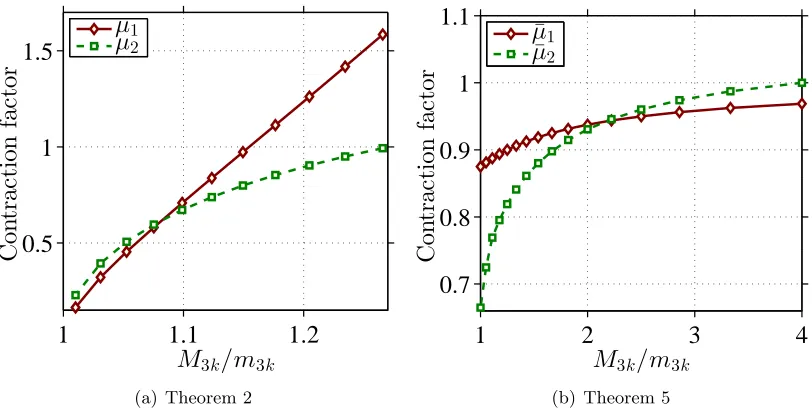
Figure 1: Evolving curves of the contraction factors in Theorem 2 and Theorem 5.
above to guarantee convergence, and be bounded away from zero to avoid early stopping as well. Similarly,M3k/m3k<1.26 in the part(b) is a necessary condition to guarantee the
existence of η such that ρ < 0.62 and µ2 < 1. Figure 1(a) shows the evolving curves of contraction factors µ1 and µ2 as functions of M3k/m3k in the interval [1,1.26). It can be
seen from this figure that µ1 < µ2 when M3k/m3k → 1 and µ1 > µ2 for relatively larger
M3k/m3k.
The non-vanishing terms in the error bounds of Theorem 2 indicate that the estimation errors of GraHTP and FGraHTP are controlled by the multiplier of√kk∇f(¯x)k∞.
Partic-ularly if the sparse vector ¯xis sufficiently close to an unconstrained minimum off, then the estimation error floor is negligible because k∇f(¯x)k∞ has small magnitude. The following
corollary is a direct consequence of Theorem 2 which shows that exact support recovery is possible when ¯xmin is significantly larger than
√
kk∇f(¯x)k∞.
Corollary 3 Assume the conditions in Theorem 2 hold.
(a) Let x¯ be an arbitrary k-sparse vector satisfying x¯min > 5.66η
√ k
1−2ρ k∇f(¯x)k∞. Then
GraHTP will output x(t) satisfying supp(x(t)) =supp(¯x) after t=lµ1
1 ln
2kx(0)−x¯k
¯
xmin
m
steps of iteration.
(b) Let x¯ be an arbitrary k-sparse vector satisfying x¯min > 5.62η
√ k
1−1.62ρk∇f(¯x)k∞. Then
FGraHTP will outputx(t)satisfying supp(x(t)) =supp(¯x)aftert=lµ1
2 ln
2kx(0)−x¯k
¯
xmin
m
steps of iteration.
Indeed, given the conditions in Corollary 3, for both GraHTP and FGraHTP we can show that kx(t)−x¯k < x¯min and thus supp(x(t)) = supp(¯x) must hold as x(t) and ¯x are both
Remark 4 Corollary 3 shows that GraHTP/FGraHTP requires RIP-type conditions as in Theorem 2 to guarantee exact support recovery. As a comparison, the existing sparsity re-covery results for`1-estimators (Wainwright, 2009; Li et al., 2015) are free of RIP-type con-ditions but instead relying on the irrepresentablility condition which is known to be stronger. For example, a case where the RIP-type condition holds while the irrepresentability condition does not was given by Van De Geer & B¨uhlmann (2009, Example 10.4).
The RIP-type conditions assumed in Theorem 2 could still be restrictive in real-life high-dimensional statistical settings wherein pairs of variables can be arbitrarily correlated. In the following theorem, we further show that by properly relaxing sparsity levels, GraHTP and FGraHTP are able to accurately estimate parameters without assuming bounded re-stricted strong condition numbers. A proof of this theorem is deferred to Appendix B.2.
Theorem 5 Let x¯be an arbitraryk¯-sparse vector withk¯≤k. Assume thats= 2k+ ¯k < p.
(a) Assume that f is M2k-smooth and m2k-strongly convex. Assume the step-size η <
1/M2k. If k≥
2 +η2m42 2k
¯
k, then GraHTP outputsx(t) satisfying
kx(t)−x¯k ≤
s
2¯µt14¯(0)
m2k
+2.83
√
kk∇f(¯x)k∞
m2k
,
where µ¯1 = 1−ηm2k(1−ηM2k)/2 and 4¯(0) = max{f(x(0))−f(¯x),0}.
(b) Assume that f is Ms-smooth and ms-strongly convex. Assume the step-size η <
2ms/Ms2 such that ρ= p
1−2ηms+η2Ms2 <1. If k > ρk/¯ (1−ρ)2, then FGraHTP
outputs x(t) satisfying
kx(t)−x¯k ≤µ¯t2kx(0)−x¯k+ γη
√
s 1−µ¯2
k∇f(¯x)k∞,
where µ¯2 =ργ∈(0,1)and γ =
r
1 +k/k¯ +p(4 + ¯k/k)¯k/k/2.
Remark 6 When using step-size η = 2M1
2k, the part(a) of Theorem 5 tells that GraHTP
converges linearly towards an arbitrary ¯k-sparse vector x¯ if the sparsity level is chosen as
k ≥ 2 +16M2k2
m2 2k
¯
k. The estimation error is controlled by the multiplier of √kk∇f(¯x)k∞.
Similarly, the part(b) of Theorem 5 establishes the convergence result of FGraHTP with proper relaxedkk¯. Note that the condition k > ρk/¯ (1−ρ)2 in part(b) actually enforces the contraction factor µ¯2 <1. Figure 1(b) shows the evolving curves of contraction factors ¯
µ1 andµ¯2 as functions of M3k/m3k, with the same target sparsity¯k. We can see from this
figure thatµ¯2 is superior to µ¯1 when M3k/m3k is relatively small.
(a) Under the conditions in Theorem 5(a), if x¯min > 5.66
√ k
m2k k∇f(¯x)k∞, then GraHTP
will output x(t) satisfying supp(¯x) ⊆ supp(x(t)) after t =
l
1 ¯
µ1 ln
8 ¯4(0)
m2k¯x2min
m
steps of iteration.
(b) Under the conditions in Theorem 5(b), if x¯min > 2γη
√ s
1−µ¯2 k∇f(¯x)k∞, then FGraHTP
will output x(t) satisfying supp(¯x) ⊆ supp(x(t)) after t =
l
1 ¯
µ2 ln
2kx(0)−x¯k
¯
xmin
m
steps of iteration.
Indeed, the conditions in Corollary 7 imply kx(t)−x¯k < x¯min which leads to supp(¯x) ⊆ supp(x(t)). We note that the parameter estimation error bound derived by Jain et al. (2014, Theorem 3) implies a similar support recovery guarantee as in Corollary 7(a).
3.2 Comparison to Prior Results
Now we compare our method and parameter estimation error bounds to some prior relevant methods and results.
Our method versus nonlinear-IHT (Blumensath, 2013). As we remarked in Section 2 that FGraHTP is identical to the nonlinear-IHT method proposed by Blumensath (2013). The estimation error results of the two, however, are different: the error bound of nonlinear-IHT is relying on the objective value at the target solution; whereas ours in Theorem 2(b) is controlled by the infinity norm of gradient at the target solution.
Our method versus `1-norm ball constrained estimation (Agarwal et al., 2012). It is worthwhile to compare our`0-estimation results to those established by Agar-wal et al. (2012, Theorem 1) for`1-norm ball constrained M-estimator (maximum likelihood type estimator). Let us consider ¯xas the underlying ¯k-sparse nominal parameter in a statis-tical model. When using sparsity levelk= ¯k, theO(√kk∇f(¯x)k∞) estimation error bound
in Theorem 2, which is at the same order of statistical error, is essentially identical to the error bound derived by Agarwal et al. (2012, Theorem 1). Our analysis, however, requires a bounding assumption on the restricted strong condition number which is not required in their result. This can be interpreted as the price of using nonconvex sparsity constraint rather than its convex relaxation. By using properly relaxed sparsity levelk=O(¯k), we ob-tain similar estimation error bounds in Theorem 5 but without assuming bounded restricted strong condition number. In this case, at a slight sacrifice in sparsity level, our methods gain better dependence on restricted strong condition number than those for convex models. Concerning the efficiency of projection steps, the `0-projection used in FGraHTP is more efficient than the `1-projection required by those first-order convex minimization methods. The projection operation of GraHTP is more expensive as it requires an additional debiasing step right after `0-projection.
Although having similar convergence behavior, the per-iteration cost of GraHTP is cheaper than GraSP: at each iteration, GraSP needs to minimize the objective over a support of size at least 2k while that size for GraHTP is k. FGraHTP is even cheaper for iteration as it does not need any debiasing operation. We will compare the actual numerical performance of these methods in the experiment section.
Our results versus the results obtained by Jain et al. (2014). The RIP-condition-free estimation error bound in Theorem 5(a) has also been proved by Jain et al. (2014, Theorem 3) with relaxed sparsity levels. As pointed out in Remark 6, the contrac-tion factor ¯µ1 derived in Theorem 5(a) is inferior to the rate ¯µ2 in Theorem 5(b) when the restricted strong condition number is relatively small. Moreover, from Figure 1(b) we can see that ¯µ1 is valued in a quite restrictive interval (0.87,1) while ¯µ2 can be varied in a much wider range of (0.65,1). Figure 1(a) shows that the contraction factorsµ1andµ2 derived in Theorem 2 can be widely valued in (0,1). The more favorable contraction factors in Theo-rem 5(b) and TheoTheo-rem 2 are resulted from a more careful analysis of GraHTP/FGraHTP and using a tight hard-thresholding bound derived by Shen & Li (2016).
4. Sparsity Recovery Analysis
In this section, we further analyze the sparsity recovery performance of GraHTP. In Corol-lary 3 and CorolCorol-lary 7, we have already established some general sparsity recovery results for GraHTP. Here we will provide a refined analysis without assuming bounded restricted strong condition number. Moreover, we will analyze the sparsity recovery behavior of the sparse estimator x? = arg minkxk0≤kf(x) which to our knowledge has not been addressed
elsewhere in literature. The main results obtained in this section are highlighted in below:
• For GraHTP algorithm, we derive in Theorem 8 an improved RIP-condition-free result for exactly recovering the support of a target ¯k-sparse vector with ¯k < k.
• For the global k-sparse minimizer x?, we provide in Theorem 10 a set of sufficient conditions under whichx? is able to recover the support of a target sparse vector.
4.1 Sparsity Recovery of GraHTP
In the following theorem, we show that for proper k > ¯k, GraHTP is able to recover the support of certain target ¯k-sparse vector without assuming bounded restricted strong condition numbers. A proof of this theorem is given in Appendix C.1.
Theorem 8 Assume thatf is M2k-smooth and m2k-strongly convex. Let x¯ be an arbitrary
¯
k-sparse vector satisfying k ≥1 +16M2k2
m2 2k
¯
k. Set the step-size to be η = 2M1
2k. If x¯min >
2.3
q
f(¯x)−f(x?)
m2k , then GraHTP will terminate and output x
(t) satisfying supp(x(t),k¯) = supp(¯x) after at most
t=
&
2kM2k
m2k
ln4 (0)
4−? '
steps of iteration, where 4(0)=f(x(0))−f(x?) and
4−?= min
kxk0≤k,supp(x)6=supp(x?),f(x)>f(x?)
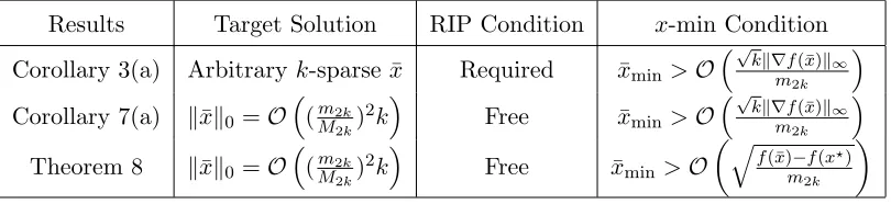
Results Target Solution RIP Condition x-min Condition
Corollary 3(a) Arbitrary k-sparse ¯x Required x¯min>O
√
kk∇f(¯x)k∞
m2k
Corollary 7(a) kx¯k0=O
(m2k
M2k)
2k Free x¯
min>O
√
kk∇f(¯x)k∞
m2k
Theorem 8 kx¯k0=O(m2k
M2k)
2k Free x¯
min >O
q
f(¯x)−f(x?)
m2k
Table 2: Comparison of Theorem 8 against Corollary 3 and Corollary 7.
Remark 9 The main message conveyed by Theorem 8 is: Ifk¯=Om22k
M2 2k
k
and the nonzero
elements in x¯ are significantly larger than the value p(f(¯x)−f(x?))/m
2k, then GraHTP
will output x(t) whose top ¯k entries are exactly the supporting set of x¯. The implication of this result is that in order to recover certain ¯k-sparse signals, one may run GraHTP with a properly relaxed sparsity level kuntil convergence and then preserve the top ¯kentries of the
k-sparse output as the final estimation.
In Table 2, we summarize the sparsity recovery results established in Theorem 8, Corol-lary 3 and CorolCorol-lary 7. We claim that the x-min condition in Theorem 8 is no stronger than those in Corollary 3 and Corollary 7. Indeed, when ¯x 6= x?, from the restricted strong-convexity off and the fact x>y≤ kxk∞kyk1 we can derive the following inequality:
f(¯x)−f(x?)≤ k∇f(¯x)k
2
∞kx¯−x?k21
2m2kkx¯−x?k2
.
It can be verified that the factor ¯l=kx¯−x?k2
1/kx¯−x?k2 is valued in the interval [1, k+ ¯k] if ¯x6= x?. Since k > ¯k, we then always have p(f(¯x)−f(x?))/m
2k ≤ √
kk∇f(¯x)k∞/m2k.
The closer ¯lis to 1, the weaker lower bound condition can be imposed on ¯xminin Theorem 8. In the extreme case when ¯l = 1, the ¯xmin condition becomes ¯xmin > O(k∇f(¯x)k∞/m2k)
which is not dependent on factor √k and thus is weaker than those in Corollary 3 and Corollary 7.
4.2 Sparsity Recovery of x?
Given a target solution ¯x, the following result gives some sufficient conditions under which the sparse estimator x? is able to exactly recover the supporting set of ¯x. A proof of this result is provided in Appendix C.2.
Theorem 10 Assume thatf isM2k-smooth andm2k-strongly convex. Letx¯be an arbitrary
¯
k-sparse vector with ¯k ≤ k. Then supp(¯x) = supp(x?,k¯) if either of the following two conditions holds:
(1) x¯min > 4.59
√ k
m2k k∇f(¯x)k∞;
(2) k≥1 +4M2k2
m2 2k
¯
k andx¯min>2.3
q
f(¯x)−f(x?)
Remark 11 Theorem 10 shows that when using sparsity level k ≥ k¯, the top k¯ entries of the k-sparse global minimizer x? is exactly the support of x¯ if x¯min is significantly larger than √kk∇f(¯x)k∞/m2k. By using a more relaxed sparsity level as in condition (2),
the top k¯ entries of x? is exactly the support of x¯ when x¯min is significantly larger than
p
(f(¯x)−f(x?))/m
2k. Note that Theorem 10 is valid without imposing bounding
assump-tions on restricted strong condition number.
We now compare the support recovery result in Theorem 10 for the `0-estimator (1) to those known for the following`1-regularized estimator:
min
x∈Rpf(x) +λkxk1, (4)
wheref(x) is a convex loss function andλis the regularization strength parameter. When the loss function is quadratic, a set of sufficient conditions were derived by Wainwright (2009) to guarantee exact sparsity recovery of Lasso-type estimators. For more general loss functions, a unified sparsity recovery analysis was presented in the paper of Li et al. (2015). We summarize in below a comparison between Theorem 10 and those sparsity recovery results for `1-regularized estimators (Li et al., 2015) with respect to several key conditions:
• Local structured smoothness/convexity condition: Theorem 10 only requires first-order local structured smoothness/convexity conditions (i.e., RSC/RSS) while the results obtained by Li et al. (2015, Theorem 5.1, Condition 1) rely on certain second-order and third-order local structured smoothness conditions.
• Irrepresentablility condition: Theorem 10 is free of the so called irrepresentablility condition which is typically required to guarantee the sparsistency of `1-regularized estimators (Li et al., 2015, Theorem 5.1, Condition 3).
• x-min condition: Comparing to the x-min condition derived by Li et al. (2015, Theorem 5.1, Condition 4) which is of order O(√kk∇f(¯x)k∞), the x-min condition (1) in Theorem 10 is comparable at the same order while the x-min condition (2) is sharper since pf(¯x)−f(x?)/m
2k≤ √
kk∇f(¯x)k∞/m2k.
We comment that the above key differences also apply to the comparison between Theorem 8 for GraHTP and the sparsity recovery results for`1-regularized estimators. In Section 5.1, we will further specify our results to the setting of sparse linear regression and make a comparison against those sparsity recovery results for Lasso-type estimators (Wainwright, 2009).
5. Applications to Sparsity-Constrained M-estimation
We now specify GraHTP and its analysis to the M-estimation problem which is a popular formulation in statistical machine learning. Given a set ofnindependently drawn data sam-ples {x(i)}n
i=1, the M-estimation problem is defined as to minimize the following empirical risk function averaged over the samples:
f(w) = 1 n
n X
i=1
whereφis a loss function andwis a set of adjustable parameters. The sparsity-constrained M-estimation problem is then given by
min
w f(w), subject tokwk0 ≤k. (5)
In the subsections to follow, we will consider three instances of this model: linear regression, logistic regression and Gaussian precision matrix estimation.
5.1 Sparsity-constrained Linear Regression
Given a ¯k-sparse parameter vector ¯w, we assume the samples are generated according to the linear model v(i) = ¯w>u(i)+ε(i) where ε(i) are n i.i.d. sub-Gaussian random variables with parameterσ. The sparsity-constrained least squares regression model is then given by
min
w f(w) =
1 2n
n X
i=1
kv(i)−w>u(i)k2, subject to kwk0 ≤k. (6)
In this case, GraHTP (and FGraHTP) reduces to the conventional HTP (and IHT) of which the parameter estimation performance has been extensively studied in compressed sensing (Foucart, 2011; Blumensath & Davies, 2009). Here we illustrate the sparsity recov-ery results we established in Section 4 and compare them against those for `1-estimators. Supposeu(i) are drawn from Gaussian distribution with covariance matrix Σ0. Then it holds with high probability thatf(w) has RSC constant m2k≥λmin(Σ)− O(¯klogp/n) and RSS constant M2k ≤ λmax(Σ) +O(¯klogp/n), andk∇f( ¯w)k∞ = O
σplogp/n
. Assume
that k ≥ k¯. We summarize in below the implications of our sparsity recovery results in sparse linear regression:
• Sparsity recovery of GraHTP. Corollary 3 shows that if ¯wmin >O
σ√klogp/n λmin(Σ)
and
λmax(Σ)
λmin(Σ) is well upper bounded, then after sufficient iteration GraHTP and FGraHTP
withk= ¯kwill guarantee support recovery supp(x(t)) = supp(¯x) with high probability. Corollary 7 indicates that when using certain relaxed sparsity levelk=Oλ2max(Σ)
λ2
min(Σ)
¯ k,
GraHTP and FGraHTP are able to guarantee supp(x(t)) ⊇ supp(¯x) without as-suming bounded condition number. Since f(¯x) − f(x?) ≤ ¯lk∇f(¯x)k2∞
2m2k where ¯l = kx¯−x?k2
1/kx¯−x?k2∈[1, k+ ¯k], Theorem 8 implies that if ¯wmin >O
σ√¯llogp/n λmin(Σ)
and
k= Oλ2max(Σ)
λ2
min(Σ)
¯
k, then after finite iteration GraHTP will guarantee supp(x(t),k¯) = supp(¯x) with high probability.
• Sparsity recovery of the least squares estimator (6). Let w? be the global k-sparse minimizer of (6). Theorem 10 shows that supp(w?,k¯) = supp( ¯w) holds with high
probability if ¯wmin >O
σ√klogp/n λmin(Σ)
. To compare our sparsity recovery results for
`0-estimators against those established by Wainwright (2009, Theorem 1) for Lasso-type estimators, the signal-noise-ratio condition of ¯wmin >O
σ√klogp/n λmin(Σ)
in that paper. The key difference is that our analysis is valid without imposing the irrepresentablility condition on design matrix which is required in the sparsity recovery analysis of Lasso-type estimators.
5.2 Sparsity-constrained Logistic Regression
Logistic regression is one of the most popular models in statistical machine learning (Bishop, 2006). In this model the relation between the random feature vector u ∈ Rp and its
associated random binary label v∈ {−1,+1}is determined by the conditional probability
P(v|u; ¯w) = exp(2vw¯
>u)
1 + exp(2vw¯>u), (7)
where ¯w ∈ Rp denotes parameter vector. Given a set of n independently drawn data
samples {(u(i), v(i))}n
i=1, logistic regression learns the parameters so as to minimize the following logistic loss function:
l(w) :=−1
nlog
Y
i
P(u(i)|v(i);w) = 1 n
n X
i=1
log(1 + exp(−2v(i)w>u(i))),
which is known to be convex. Unfortunately, in high-dimensional setting, i.e., n < p, the problem can be underdetermined and thus its minimum is not unique. A conventional way to handle this issue is to impose `2-regularization to the logistic loss to avoid singularity. The `2-penalty, however, does not promote sparse solutions which are often desirable in high-dimensional learning tasks. The sparsity-constrained`2-regularized logistic regression is then given by
min
w f(w) =l(w) +
λ 2kwk
2, subject to kwk
0 ≤k, (8)
whereλ >0 is the regularization strength parameter. Obviouslyf(w) isλ-strongly convex. The cardinality constraint enforces the solution to be sparse.
Verifying restricted smoothness and strong convexity. Let U = [u(1), ..., u(n)]∈
Rp×nbe the design matrix andσ(z) = 1/(1 + exp(−z)) be the sigmoid function. In the case of`2-regularized logistic loss considered in this section we have ∇f(w) =U a(w)/n+λw in which the vectora(w)∈Rnis given by [a(w)]i =−2v(i)(1−σ(2v(i)w>u(i))), and the Hessian ∇2f(w) =UΛ(w)U>/n+λI where Λ(w) is ann×ndiagonal matrix whose diagonal entries
[Λ(w)]ii= 4σ(2viw>ui)(1−σ(2viw>ui)). Given an integers, recall thatλmax(A, s) denotes the largest s-sparse eigenvalue of a positive semi-definite matrix A and λmin(A, s) denotes the smallests-sparse eigenvalue ofA. Assume that the algorithm is initialized with all-zero vector. Then it can be verified thatf(w) is (λmax(U U>, s)+λ)-smooth and (γs+λ)-strongly
convex whereγs := minf(w)≤f(0)λmin(UΛ(w)U>, s).
Bounding the value of k∇f( ¯w)k∞. We now bound the infinity norm k∇f( ¯w)k∞
which controls the estimation error and sparisty recovery bounds of GraHTP/FGraHTP. In the following derivation, we assume that the joint density of the random vector (u, v)∈Rp+1 is given by the following exponential family distribution:
P(u, v; ¯w) = exp
vw¯>u+B(u)−A( ¯w)
where
A( ¯w) := log X
v={−1,1}
Z
Rp
expvw¯>u+B(u)du
is the log-partition function. The term B(u) characterizes the marginal behavior of u. Obviously, the conditional distribution of v given u, P(v | u; ¯w), is given by the Bernoulli distribution in (7). By doing some elementary manipulations (see, e.g., Wainwright & Jor-dan, 2008) we can obtain the following standard result which shows that the first derivative of the logistic log-likelihoodl(w) yields the cumulants of the random variablesv[u]j:
∂l ∂[w]j
= 1 n
n X
i=1
n
−v(i)[u(i)]j+Ev[v[u(i)]j |u(i)] o
. (10)
Here the expectation Ev[· |u] is taken over the conditional distribution (7). We introduce
the following sub-Gaussian condition on the random variate v[u]j.
Assumption 1 For all j, we assume that there exists constantσ >0 such that for all ζ,
E[exp(ζv[u]j)]≤exp σ2ζ2/2
.
This assumption holds when [u]j are sub-Gaussian (e.g., Gaussian or bounded) random
variables. The following result establishes the bound ofk∇f( ¯w)k∞.
Proposition 12 If Assumption 1 holds, then with probability at least 1−4p−1,
k∇f( ¯w)k∞≤4σ
p
lnp/n+λkw¯k∞.
A proof of this result is provided in Appendix D.1. If we choose λ = O(plnp/n), then with overwhelming probabilityk∇f( ¯w)k∞vanishes at the rate of O(
p
lnp/n). This bound is superior to the bound obtained by Bahmani et al. (2013, Section 4.2) which is not van-ishing as sample size increases. Based on the above discussion, we can similarly specify our parameter estimation and sparsity recovery results to sparse logistic regression. Here we omit the detailed specification of results for the sake of redundance reducing.
5.3 Sparsity-constrained Gaussian Precision Matrix Estimation
As an important class of sparse learning problems for exploring the interrelationship among a large number of random variables, the sparse Gaussian precision (inverse covariance) matrix estimation problem has received significant interest in a variety of scientific and engineering domains, including computational biology, natural language processing and document analysis.
Let x be a p-variate random vector with zero-mean Gaussian distribution N(0,Σ). Its¯ density is parameterized by the precision matrix ¯Ω = ¯Σ−1 0 as
φ(x; ¯Ω) = p 1
(2π)p(det ¯Ω)−1 exp
−1
2x
>¯
Ωx
.
components of x, on the other hand, can be represented by a graph G = (V, E) in which the vertex setV has p elements corresponding to [x]1, ...,[x]p, and the edge setE consists
of edges between node pairs {[x]i,[x]j}. The edge between [x]i and [x]j is excluded from
E if and only if [x]i and [x]j are conditionally independent given other variables. This
graphical model is known as Gaussian Markov random field (GMRF) (Edwards, 2000). Thus for multivariate Gaussian distribution, estimating the support of the precision matrix
¯
Ω is equivalent to learning the structure of GMRFG.
Given i.i.d. samples Xn={x(i)}ni=1 drawn fromN(0,Σ), the negative log-likelihood, up¯ to a constant, can be written in terms of the precision matrix as
L(Xn; ¯Ω) :=−log det ¯Ω +hΣn,Ω¯i,
where Σn is the sample covariance matrix. We are interested in the problem of estimating
a sparse precision ¯Ω with no more than a pre-specified number of off-diagonal nonzero entries. For this purpose, we consider the following cardinality constrained log-determinant program:
min
Ω0L(Ω) :=−log det Ω +hΣn,Ωi, s.t. kΩ
−k
0 ≤2k, (11)
where Ω− is the restriction of Ω on the off-diagonal entries, kΩ−k0 = |supp(Ω−)| is the cardinality of the supporting set of Ω− and the integerk >0 controls the number of edges, i.e., |E|, in the graph.
Verifying restricted smoothness and strong convexity. It can be verified that the Hessian matrix of L(Ω) is given by ∇2L(Ω) = Ω−1⊗Ω−1, where ⊗denotes the Kronecker product operator. Suppose that kΩ−k0 ≤ s and αsI Ω βsI for some 0 < αs ≤ βs.
Due to the fact that the eigenvalues of Kronecker products of symmetric matrices are the products of the eigenvalues of their factors, it holds that βs−2I Ω−1 ⊗Ω−1 α−s2I. Therefore we haveβs−2≤ k∇2L(Ω)k ≤α−2
s which implies thatL(Ω) isβ−s2-strongly convex
andα−s2-smooth. Inspired by this property, we consider applying GraHTP to the following variant of problem (11):
min
αIΩβIL(Ω), s.t. kΩ
−k
0 ≤2k, (12)
where 0< α≤β are two constants which respectively lower and upper bound the eigenval-ues of the desired solution. To roughly estimateα andβ, we employ a rule proposed by Lu (2009, Proposition 3.1) for the`1-regularized log-determinant program. Specifically, we set
α= (kΣnk2+nξ)−1, β =ξ−1(n−αTr(Σn)),
whereξ is a small enough positive number (e.g.,ξ= 10−2 as used in our implementation). Bounding the value of |∇L( ¯Ω)|∞. It is standard to know that |∇L( ¯Ω)|∞ =|Σn−
¯
Σ|∞=O(
p
logp/n) with probability at least 1−c0p−c1 for some positive constantsc0 and
c1 and sufficiently large n (see, e.g., Ravikumar et al., 2011, Lemma 1). Therefore, with overwhelming probability we have |∇L( ¯Ω)|∞=O(
p
constraint. To address this issue, we need to accordingly modify the debiasing step (S3) of GraHTP to minimizeL(Ω) over the constraints αIΩβI and supp(Ω)⊆F(t):
min
αIΩβIL(Ω), s.t. supp(Ω)⊆F
(t). (13)
Since this problem is convex, any off-the-shelf convex solver can be applied for optimiza-tion. In our implementation, we resort to the alternating direction method of multipliers (ADMM) (Boyd et al., 2010; Yuan, 2012) which has been observed to be efficient in our numerical practice. The implementation details of ADMM for solving the subproblem (13) are deferred to Appendix D.2. The modified GraHTP for sparse Gaussian precision matrix estimation is outlined in Algorithm 2.
Algorithm 2:A Modified GraHTP for Sparse Gaussian Precision Matrix Estimation.
Initialization: Ω(0) with k(Ω(0))−k0≤2kand αI Ω(0)βI (typically Ω(0) =αI),
t= 1.
Output: Ω(t). repeat
(S1) Compute ˜Ω(t)= Ω(t−1)−η∇L(Ω(t−1));
(S2) Let ˜F(t)= supp(( ˜Ω(t))−,2k) be the indices of ( ˜Ω(t))− with the largest 2k absolute values andF(t)= ˜F(t)∪ {(1,1), ...,(p, p)};
(S3) Compute Ω(t)= arg minL(Ω);αIΩβI,supp(Ω)⊆F(t) ; t=t+ 1;
until halting condition holds;
6. Experimental Results
This section is devoted to illustrating the empirical performance of GraHTP/FGraHTP when applied to sparse learning tasks. Our algorithms are implemented in Matlab 7.12 running on a desktop with Intel Core i7 3.2G CPU and 16G RAM.
6.1 Sparsity-constrained Linear Regression
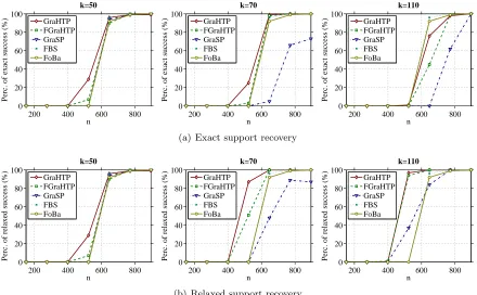
We conduct a group of Monte-Carlo simulation experiments on sparse linear regression model to verify the sparsity recovery results presented in Section 4.
Data generation. We consider a synthetic data model in which the sparse parameter ¯
wis ap= 500 dimensional vector that has ¯k= 50 nonzero entries drawn independently from a Gaussian distribution with significant mean. Each data sampleuis a normally distributed dense vector. The responses are generated byv= ¯w>u+εwhereεis a standard Gaussian noise. We allow the sample size n to be varying and for each n, we generate 100 random copies of data independently.
200 300 400 500 0 20 40 60 80 100 n
Perc. of exact success (%)
k=50 GraHTP FGraHTP GraSP FBS FoBa
200 300 400 500
0 20 40 60 80 100 n
Perc. of exact success (%)
k=70 GraHTP FGraHTP GraSP FBS FoBa
200 300 400 500
0 20 40 60 80 100 n
Perc. of exact success (%)
k=110 GraHTP FGraHTP GraSP FBS FoBa
(a) Exact support recovery
200 300 400 500
0 20 40 60 80 100 n
Perc. of relaxed success (%)
k=50 GraHTP FGraHTP GraSP FBS FoBa
200 300 400 500
0 20 40 60 80 100 n
Perc. of relaxed success (%)
k=70 GraHTP FGraHTP GraSP FBS FoBa
200 300 400 500
0 20 40 60 80 100 n
Perc. of relaxed success (%)
k=110 GraHTP FGraHTP GraSP FBS FoBa
(b) Relaxed support recovery
Figure 2: Sparse linear regression on simulated data: chance of success curves for support recovery under varying sample size and sparsity level.
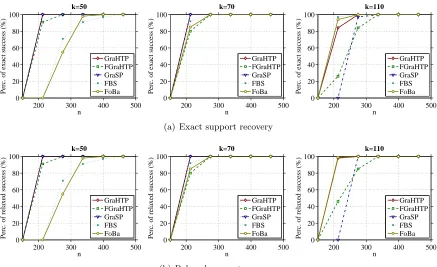
simultaneously selects at each iteration k nonzero entries and update their values via ex-ploring the topkentries in the previous iterate as well as the top 2kentries in the previous gradient. FBS is a forward-selection-type method which iteratively selects an atom from the dictionary and minimizes the objective function over the linear combinations of all the selected atoms. FoBa is an adaptive forward-backward greedy selection algorithm which al-lows elimination of selected variables when the objective value does not increase significantly. We use two metrics to measure the support recovery performance. We say arelaxed support recovery is successful if supp( ¯w) ⊆ supp(w(t)) and an exact support recovery is successful if supp( ¯w) = supp(w(t),¯k). We replicate the experiment over the 100 trials and record the percentage of relaxed success and percentage of exact success for each configuration of the pair (n, k).
Results. Figure 2 shows the percentage of exact (relaxed) success curves as functions of sample sizen, under different sparsity levelsk∈ {50,70,110}. From these curves we can make the following observations:
• For each curve, the chance of success increases as sample size n increases. This is as expected because the larger sample size is, the easier the x-min conditions can be fulfilled so as to guarantee exact support recovery;
conducted in GraHPT can significantly improve the accuracy of sparsity recovery, especially in noisy settings.
• The left panel of Figure 2 shows that when k = ¯k, GraHTP/FGraHTP and GraSP are comparable and they all significantly outperform FBS and FoBa, especially when the sample size is relatively small. This observation suggests that hard-thresholding-type methods are more accurate than forward and/or backward selection methods for sparsity recovery with exact sparsity level. The middle panel shows that for slightly increased sparsity levelk= 70, GraHTP and GraSP still exhibit superior performance, while the performance gap among all the considered algorithms decreases. From the right panel we can see that for relatively large k >¯k, FBS, Foba and GraHTP have much better performance than FGraHTP and GraSP.
From the above observations we conclude that GraHTP is able to achieve better trade-off between accuracy and stability of sparsity recovery than the other considered methods.
6.2 Sparsity-constrained Logistic Regression
We present in this subsection the experimental results on several synthetic and real-data sparse logistic regression tasks.
6.2.1 Monte-Carlo simulation
In this group of Monte-Carlo experiments, we use a simulated data to verify the spar-sity recovery performance of GraHTP and FGraHTP on logistic regression model. The sparse parameter and design matrix are generated in an identical way to that of the lin-ear regression model. The data labels, v ∈ {−1,1}, are generated randomly according to the Bernoulli distribution P(v = 1|u; ¯w) = exp(2 ¯w>u)/(1 + exp(2 ¯w>u)). The same ex-periment protocol as used in the previous linear regression setting applies here. Inspired by Theorem 8 and the discussion in Section 5.2, we set the step-size η = 2M1
2k where M2k = λmax(U U>,2k) +λ. The sparse eigenvalue λmax(U U>,2k) can be computed using the truncated power method (Yuan & Zhang, 2013).
Results. For different sparsity levelsk≥k¯, Figure 3 shows the chance of exact (relaxed) success curves as functions of sample size n. Again, from these curves we can observe that: 1) in a wide range of sparsity level, GraHP achieves better trade-off between accuracy and stability than the other considered sparsity recovery methods; and 2) GraHTP consistently outperforms FGraHTP in noisy settings when using k >k¯.
6.2.2 Real data experiments
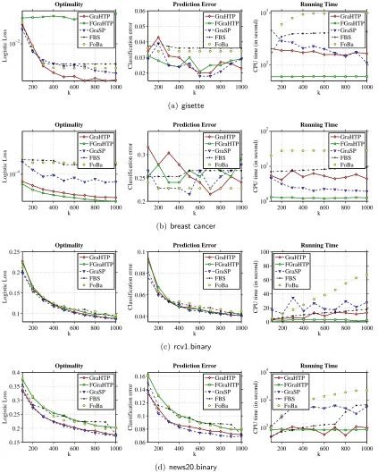
We further illustrate the performance of GraHTP/FGraHTP on real data for binary logistic regression. The data used for evaluation include twodense data setsgisette (Guyon et al., 2005) andbreast cancer(Hess et al., 2006), and twosparsedata setsrcv1.binary(Lewis et al., 2005) and news20.binary (Keerthi & DeCoste, 2005). Table 3 summaries the statistics of these data sets. For each data set, we test with sparsity parametersk∈ {100,200, ...,1000}
200 400 600 800 0 20 40 60 80 100 n
Perc. of exact success (%)
k=50 GraHTP FGraHTP GraSP FBS FoBa
200 400 600 800
0 20 40 60 80 100 n
Perc. of exact success (%)
k=70 GraHTP FGraHTP GraSP FBS FoBa
200 400 600 800
0 20 40 60 80 100 n
Perc. of exact success (%)
k=110 GraHTP FGraHTP GraSP FBS FoBa
(a) Exact support recovery
200 400 600 800
0 20 40 60 80 100 n
Perc. of relaxed success (%)
k=50 GraHTP FGraHTP GraSP FBS FoBa
200 400 600 800
0 20 40 60 80 100 n
Perc. of relaxed success (%)
k=70 GraHTP FGraHTP GraSP FBS FoBa
200 400 600 800
0 20 40 60 80 100 n
Perc. of relaxed success (%)
k=110 GraHTP FGraHTP GraSP FBS FoBa
(b) Relaxed support recovery
Figure 3: Sparse logistic regression on simulated data: chance of success curves for support recovery under varying sample size and sparsity level.
Datasets Training Size Testing Size Dimensionality
gisette 6,000 1,000 5,000
breast cancer 54 79 22,283
rcv1.binary 20,242 20,000 47,236
news20.binary 10,000 9,996 1,355,191
Table 3: Statistics of data sets used in binary logistic regression experiment.
Results. The objective value, test classification error and CPU running time curves under varying sparsity levelkare plot in Figure 4. From these curves we have the following observations:
• On optimality: GraHTP is superior to the other considered algorithms in most cases. FGraHTP is less optimal ongisettedata, while it is comparable to the other algorithms on the other three data sets.
200 400 600 800 1000 10−2 k Logistic Loss Optimality GraHTP FGraHTP GraSP FBS FoBa
200 400 600 800 1000
0.02 0.03 0.04 0.05 0.06 k Classification error Prediction Error GraHTP FGraHTP GraSP FBS FoBa
200 400 600 800 1000
102
103
k
CPU time (in second)
Running Time GraHTP FGraHTP GraSP FBS FoBa (a)gisette
200 400 600 800 1000
10−4 k Logistic Loss Optimality GraHTP FGraHTP GraSP FBS FoBa
200 400 600 800 1000
0.2 0.25 0.3 k Classification error Prediction Error GraHTP FGraHTP GraSP FBS FoBa
200 400 600 800 1000
100
101
102
k
CPU time (in second)
Running Time GraHTP FGraHTP GraSP FBS FoBa
(b) breast cancer
200 400 600 800 1000
0.1 0.15 0.2 0.25 k Logistic Loss Optimality GraHTP FGraHTP GraSP FBS FoBa
200 400 600 800 1000
0.04 0.06 0.08 0.1 k Classification error Prediction Error GraHTP FGraHTP GraSP FBS FoBa
200 400 600 800 1000
0 20 40 60 80 100 k
CPU time (in second)
Running Time GraHTP FGraHTP GraSP FBS FoBa (c) rcv1.binary
200 400 600 800 1000
0.15 0.2 0.25 0.3 0.35 0.4 k Logistic Loss Optimality GraHTP FGraHTP GraSP FBS FoBa
200 400 600 800 1000
0.06 0.08 0.1 0.12 0.14 0.16 k Classification error Prediction Error GraHTP FGraHTP GraSP FBS FoBa
200 400 600 800 1000
102
103
104
k
CPU time (in second)
Running Time GraHTP FGraHTP GraSP FBS FoBa (d) news20.binary
0.02 0.04 0.06 0.08 0.1 0 0.05 0.1 λ Classification error Prediction Error GraHTP FGraHTP Lasso−APG
0.02 0.04 0.06 0.08 0.1 102
103
λ
CPU time (in second)
Running Time
GraHTP FGraHTP Lasso−APG
(a)gisette
2 4 6 8 10 x 10−3 0.22 0.24 0.26 0.28 0.3 0.32 λ Classification error Prediction Error GraHTP FGraHTP Lasso−APG
2 4 6 8 10
x 10−3 101
102
λ
CPU time (in second)
Running Time
GraHTP FGraHTP Lasso−APG
(b) breast cancer
2 4 6 8 10 x 10−5 0.04 0.045 0.05 λ Classification error Prediction Error GraHTP FGraHTP Lasso−APG
2 4 6 8 10
x 10−5 101
102
λ
CPU time (in second)
Running Time
GraHTP FGraHTP Lasso−APG
(c)rcv1.binary
1 2 3 4 5
x 10−4 0.05 0.1 0.15 0.2 λ Classification error Prediction Error GraHTP FGraHTP Lasso−APG
1 2 3 4 5
x 10−4 102
103
λ
CPU time (in second)
Running Time
GraHTP FGraHTP Lasso−APG
(d) news20.binary
Figure 5: Sparse logistic regression on real data: comparison between GraHTP/FGraHTP and Lasso-type estimator in classification error and CPU running time.
• On execution time: FGraHTP is the most efficient one and GraHTP is the runner-up except on breast cancer. Particularly, as shown in Figure 4(d) that the computa-tional advantage of FGraHTP/GraHTP over the other considered methods becomes significant onnews20.binary which is relatively large in scale.
To summarize, GraHTP and FGraHTP are able to achieve desirable trade-off between accuracy and efficiency on the considered data sets.
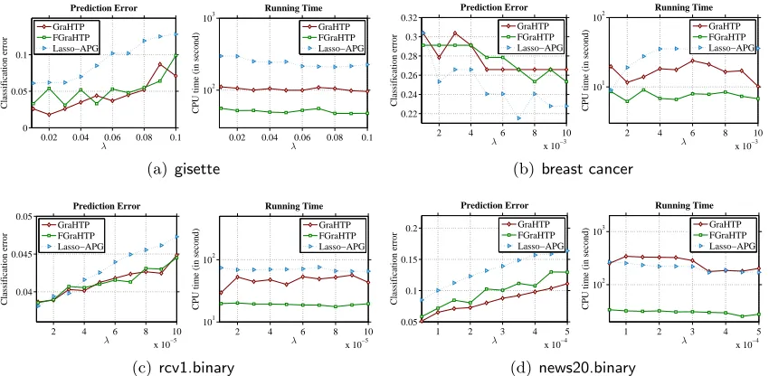
Comparison against Lasso-type estimator. We have also conducted a set of ex-periments to compare GraHTP/FGraHTP against the Lasso-type estimator (4) for `1 -regularized sparse learning. To make a fair comparison, we first solve the Lasso-type esti-mator (4) using an accelerated proximal gradient method (Beck & Teboulle, 2009), which we call LasAPG, and then run GraHTP with the sparsity level of the LasAPG so-lution. Figure 5 shows the test classification error and CPU running time curves under varying regularization parameter λ. We can observe from this group of results that: (1) GraHTP and FGraHTP outperform Lasso-APG in classification accuracy on three out of the four data sets in use; and (2) FGraHTP is the most efficient one on all the data sets and GraHTP is faster than Lasso-APG on three of the data sets. Based on these observations, we can conclude that GraHTP and FGraHTP tend to be more accurate and efficient than Lasso-type estimator when their output solutions are at the same sparsity level.
6.3 Sparsity-constrained Gaussian Precision Matrix Estimation
50 100 150 200 0
20 40 60 80 100
Dimensionality p
Frobenius norm
Estimation Error
GraHTP GraSP FBS FoBa GLasso
50 100 150 200
0.2 0.4 0.6 0.8 1
Dimensionality p
F−Score
Structure Recovery
GraHTP GraSP FBS FoBa GLasso
50 100 150 200
10−2
100
102
Dimensionality p
CPU time (in second)
Running Time
GraHTP GraSP FBS FoBa GLasso
Figure 6: Sparse precision matrix estimation on simulated data: Matrix Frobenius norm loss, support recovery F-score and CPU running time curves under varying data dimensionality. The larger the F-score, the better the support recovery perfor-mance.
6.3.1 Monte-Carlo Simulation
Our simulation study employs the sparse precision matrix model ¯Ω = Θ +σI where each off-diagonal entry in Θ is generated independently and equals 1 with probability P = 0.1 or 0 with probability 1−P = 0.9. Θ has zeros on the diagonal, and σ is chosen so that the condition number of ¯Ω is p. Let ¯Σ = ¯Ω−1 be the covariance matrix. We generate a training sample of sizen= 100 fromN(0,Σ), and an independent sample of size 100 from¯ the same distribution for tuning the parameterk. The numerical performance is evaluated with different values ofp∈ {30,60,120,200}, replicated 100 times each.
We compare the modified GraHTP (as outlined in Algorithm 2) with GraSP, FBS and FoBa. To adopt GraSP to sparse precision matrix estimation, we modify the algorithm with a similar two-stage strategy as used in the modified GraHTP such that it can han-dle the eigenvalue bounding constraint in addition to the sparsity constraint. FBS and FoBa have already been applied to sparse precision matrix estimation problems in litera-ture (Yuan & Yan, 2013; Jalali et al., 2011). Also, we compare GraHTP with Graphical Lasso (GLasso) which is one of the representative Lasso-type convex estimators for `1 -penalized log-determinant program (Friedman et al., 2008). The quality of precision matrix estimation is measured by its distance to the truth in Frobenius norm and the support recovery F-score. The larger the F-score, the better the support recovery performance.
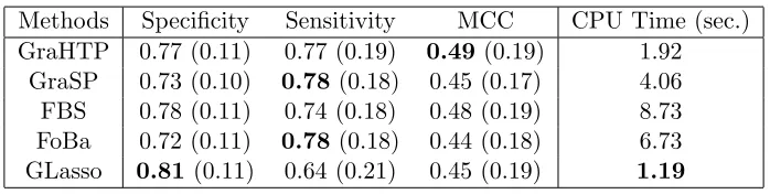
Methods Specificity Sensitivity MCC CPU Time (sec.) GraHTP 0.77 (0.11) 0.77 (0.19) 0.49 (0.19) 1.92
GraSP 0.73 (0.10) 0.78 (0.18) 0.45 (0.17) 4.06 FBS 0.78 (0.11) 0.74 (0.18) 0.48 (0.19) 8.73 FoBa 0.72 (0.11) 0.78 (0.18) 0.44 (0.18) 6.73 GLasso 0.81 (0.11) 0.64 (0.21) 0.45 (0.19) 1.19
Table 4: Sparse precision matrix estimation on breast cancer data: comparison of average (std) classification accuracy and average CPU running time over 100 replications.
6.3.2 Real Data
We consider the task of LDA (linear discriminant analysis) classification of tumors using the breast cancer data set. This data consists of 133 subjects, each of which is associated with 22,283 gene expression levels. Among these subjects, 34 are with pathological complete response (pCR) and 99 are with residual disease (RD). The pCR subjects are considered to have a high chance of cancer free survival in the long term. Based on the estimated precision matrix of the gene expression levels, we apply LDA to predict whether a subject can achieve the pCR state or the RD state.
Experiment protocol. In this experiment, we follow the same protocol as what was used in the paper of Cai et al. (2011). The data are randomly divided into the training and test sets. In each random division, 5 pCR subjects and 16 RD subjects are ran-domly selected to constitute the test data, and the remaining subjects form the training set with size n = 112. By using two-sample t test, p = 113 most significant genes are selected as covariates. Following the LDA framework, we assume that the normalized gene expression data are normally distributed as N(µl,Σ), where the two classes are as-¯
sumed to have the same covariance matrix, ¯Σ, but different means, µl, l = 1 for pCR
state and l = 2 for RD state. Given a test data sample x, we calculate its LDA scores, δl(x) =x>Ωˆˆµl− 12µˆ>l Ωˆˆµl+ log ˆπl, l = 1,2, using the precision matrix ˆΩ estimated by the
considered methods. Here ˆµl = (1/nl)Pi∈classlxi is the within-class mean in the training
set and ˆπl=nl/nis the proportion of classl subjects in the training set. The classification
rule is ˆl(x) = arg maxl=1,2δl(x). Clearly, the classification performance is directly affected
by the estimation quality of ˆΩ. Hence, we assess the precision matrix estimation perfor-mance on the test data and compare GraHTP with GraSP, FBS, FoBa and GLasso. We use a 6-fold cross-validation on the training data for tuning the sparsity level parameter in `0-estimators and the regularization strength parameter in GLasso. We replicate the experiment 100 times.
(MCC) criteria as used by Cai et al. (2011):
Specificity = TN
TN + FP, Sensitivity =
TP TP + FN,
MCC = p TP×TN−FP×FN
(TP + FP)(TP + FN)(TN + FP)(TN + FN),
where TP and TN stand for true positives (pCR) and true negatives (RD), respectively, and FP and FN stand for false positives/negatives, respectively. The larger the criterion value, the better the classification performance. Since one can adjust decision threshold in any specific algorithm to trade-off specificity and sensitivity (increase one while reduce the other), the MCC is more meaningful as a single performance metric. Table 4 lists the averages and standard deviations, in the parentheses, of the three classification criteria over 100 replications. It can be observed that GraHTP is quite competitive to the leading methods in all the three metrics. The average CPU running time of each considered method is listed in the rightmost column of Table 4.
7. Conclusion
In this article, we proposed GraHTP as a generalization of HTP from compressed sensing to the generic problem of sparsity-constrained loss minimization. The main idea is to force the gradient descent iteration to be sparse via hard thresholding. Theoretically, we proved that under mild conditions, GraHTP converges geometrically and its estimation error is controlled by the restricted norm of gradient at the target sparse solution. Under prop-erly strengthened conditions, we further established the sparsity recovery performance of GraHTP which to our knowledge has not been systematically analyzed elsewhere in liter-ature. Also, we have proposed and analyzed the FGraHTP algorithm as a fast variant of GraHTP without applying the debiasing operation after truncation. Empirically, we showed that GraHTP and FGraHTP are superior or competitive to the state-of-the-art greedy pur-suit methods when applied to sparse learning problems including linear regression, logistic regression and precision matrix estimation. To conclude, simply combining gradient descent with hard thresholding leads to an accurate and computationally tractable procedure for solving sparsity-constrained loss minimization problems.
Acknowledgments
The authors would like to thank the anonymous referees for their constructive comments which are extremely helpful for improving this work. Xiao-Tong Yuan and Ping Li were partially supported by NSF-Bigdata-1419210, NSF-III-1360971, ONR-N00014-13-1-0764, and AFOSR-FA9550-13-1-0137. Xiao-Tong Yuan is also partially supported by NSFC-61522308 and Tencent AI Lab Rhino-Bird Joint Research Program (No.JR201801). Tong Zhang was supported by NSF-IIS-1407939 and NSF-IIS-1250985.
Appendix A. Technical Lemmas
Lemma 13 Let x be a k-sparse vector andy =x−η∇f(x). Iff is M2k-smooth, then the
following inequality holds:
f(yk)≤f(x)−
1−ηM2k
2η kyk−xk
2. Proof Since f is M2k-smooth, it follows that
f(yk)−f(x)≤h∇f(x), yk−xi+
M2k
2 kyk−xk 2
ξ1
≤ − 1
2ηkyk−xk
2+ M2k
2 kyk−xk 2 =− 1−ηM2k
2η kyk−xk
2,
where “ξ1” follows from the fact thatyk is the bestk-support approximation toy such that kyk−yk2 =kyk−x+η∇f(x)k2 ≤ kx−x+η∇f(x)k2 =kη∇f(x)k2,
which implies 2ηh∇f(x), yk−xi ≤ −kyk−xk2.
Lemma 14 Assume thatf isms-strongly convex. Then for any kx−x0k0 ≤sit holds that
kx−x0k ≤
s
2 max{f(x)−f(x0),0}
ms
+ 2k∇F∪F0f(x
0)k
ms
,
where F =supp(x) and F0=supp(x0).
Proof Since f is ms-strongly convex, we have
f(x)≥f(x0) +h∇f(x0), x−x0i+ ms 2 kx−x
0k2
≥f(x0)− k∇F∪F0f(x0)kkx−x0k+ms
2 kx−x
0k2,
where the second inequality follows from Cauchy-Schwarz inequality. From this above inequality we can see that if f(x)≤f(x0), then
kx−x0k ≤ 2k∇F∪F0f(x
0)k
ms
.
If otherwisef(x)> f(x0), then we have
kx−x0k ≤k∇F∪F0f(x
0)k+p
k∇F∪F0f(x0)k2+ 2ms(f(x)−f(x0))
ms
≤2k∇F∪F0f(x
0)k+p
2ms(f(x)−f(x0))
ms
.
Lemma 15 Assume that f is ms-strongly convex and Ms-smooth. For any index set F
with cardinality |F| ≤s and any x, y with supp(x)∪supp(y)⊆F, if η∈(0,2ms/Ms2), then kx−y−η∇Ff(x) +η∇Ff(y)k ≤
p
1−2ηms+η2Ms2kx−yk,
and p1−2ηms+η2Ms2<1.
Proof By adding two copies of the inequality (2) withx andy interchanged and applying Theorem 2.1.5 in the textbook (Nesterov, 2004) on the supporting setF, we can show that
(x−y)>(∇f(x)− ∇f(y))≥mskx−yk2, k∇Ff(x)− ∇Ff(y)k ≤Mskx−yk.
Then for any η >0 we have
kx−y−η∇Ff(x) +η∇Ff(y)k2 ≤(1−2ηms+η2Ms2)kx−yk2.
It is clear that 1−2ηms+η2Ms2 ≥1−m2s/Ms2 ≥ 0. The condition η < 2ms/Ms2 implies p
1−2ηms+η2Ms2 <1. This proves the lemma.
Lemma 16 Assume that f is Ms-smooth and ms-strongly convex. Let F and F0 be two
index sets with cardinality |F ∪F0|=s. Let x = arg minsupp(y)⊆F f(y) and supp(x0) ⊆F0. Then for any η∈(0,2ms/Ms2), the following two inequalities hold:
k(x−x0)Fk ≤
ρkx0F0\Fk
1−ρ +
ηk∇F∪F0f(x0)k
1−ρ , (14)
kx−x0k ≤ kx 0 F0\Fk
1−ρ +
ηk∇F∪F0f(x0)k
1−ρ , (15)
where ρ=p1−2ηms+η2Ms2 <1.
Proof Since x is the minimum of f(y) restricted over the supporting set F, we have
h∇f(x), zi= 0 whenever supp(z)⊆F. Then
k(x−x0)Fk2
=hx−x0,(x−x0)Fi
=hx−x0−η∇F∪F0f(x) +η∇F∪F0f(x0),(x−x0)Fi −ηh∇F∪F0f(x0),(x−x0)Fi
ξ1
≤p1−2ηms+η2Ms2kx−x0kk(x−x0)Fk+ηk∇F∪F0f(x0)kk(x−x0)Fk,
where “ξ1” follows from Lemma 15. Let us abbreviate ρ =
p
1−2ηms+η2Ms2. After
simplification, we have
k(x−x0)Fk ≤ρkx−x0k+ηk∇F∪F0f(x0)k. (16)
It follows that
kx−x0k ≤k(x−x0)Fk+k(x−x0)F0\Fk
After rearrangement we obtain
kx−x0k ≤k(x−x
0)
F0\Fk
1−ρ +
ηk∇F∪F0f(x0)k
1−ρ
=
kx0F0\Fk
1−ρ +
ηk∇F∪F0f(x0)k
1−ρ .
(17)
By combining (16) and (17) we get
k(x−x0)Fk ≤
ρkx0F0\Fk
1−ρ +
ηk∇F∪F0f(x0)k
1−ρ .
This proves the desired bounds in this lemma.
The following lemma is established by Shen & Li (2016, Theorem 1) for bounding the estimation error of hard-thresholding operation. This result will be extensively used in our analysis.
Lemma 17 Let b ∈Rp be an arbitrary p-dimensional vector and a∈
Rp be any k-sparse vector. Denote k¯=kak0 ≤k. Then, we have the following universal bound:
kbk−ak2 ≤νkb−ak2, ν= 1 +
β+p(4 +β)β
2 , β =
min{k, p¯ −k}
k−¯k+ min{k, p¯ −k}.
Appendix B. Proofs of Main Theorems in Section 3
The technical proofs of main results in Section 3 are collected in this appendix section.
B.1 Proof of Theorem 2
Before proving Theorem 2, we first present two lemmas which are respectively key to the proof of part(a) and part(b) of Theorem 2.
Lemma 18 Assume thatf isM3k-smooth and m3k-strongly convex. Let x¯ be an arbitrary
k-sparse vector. Then at time instance t, for any η ∈(0,2m3k/M32k), GraHTP will output
x(t) satisfying
kx(t)−x¯k ≤ ρ
1−ρkx
(t−1)−x¯k+2ηk∇2kf(¯x)k
1−ρ ,
where ρ=
q
1−2ηm3k+η2M32k <1.
Proof Denote ¯F = supp(¯x). Since x(t) is the minimum of f(x) restricted over the sup-porting setF(t), it is directly known from the inequality (15) in Lemma 16 that
kx(t)−x¯k ≤ k(x
(t)−x¯) ¯
F\F(t)k
1−ρ +
ηk∇F(t)f(¯x)k