http://www.sciencepublishinggroup.com/j/jeee doi: 10.11648/j.jeee.20170505.17
ISSN: 2329-1613 (Print); ISSN: 2329-1605 (Online)
Analysis of Current Density in Soil for Resistivity
Measurements and Electrical Grounding Designs
Jie Liu, Farid Paul Dawalibi, Sharon Tee
Department of Research and Development, Safe Engineering Services & Technologies ltd., Laval, Canada
Email address:
[email protected] (Jie Liu)
To cite this article:
Jie Liu, Farid Paul Dawalibi, Sharon Tee. Analysis of Current Density in Soil for Resistivity Measurements and Electrical Grounding Designs. Journal of Electrical and Electronic Engineering. Vol. 5, No. 5, 2017, pp. 198-208. doi: 10.11648/j.jeee.20170505.17
Received: November 15, 2017; Accepted: November 22, 2017; Published: December 6, 2017
Abstract:
The design of electrical grounding systems is crucial to ensure people's safety and equipment integrity. The performance of the grounding system is critically dependent on the characteristics of the local soil surrounding the grounding system. Some wrong concepts and assumptions on soil electrical properties are still prevalent among professionals regarding soil resistivity measurements and grounding designs. The objective of this paper is to examine the current density in the earth surrounding measurement electrodes and electrical grounding systems and discuss the effects of soil structures on measurements and grounding related studies. The analyses described here are based on electromagnetic field theory. First, this paper examines soil resistivity measurements using the Wenner method in three typical, but different soil structure models, by exploring the distribution of earth current density in the soil surrounding the current injection electrodes. The computed results are illustrated using appropriate plots to understand better the influence of soil structure and characteristics on the current penetration across the soil layers. Furthermore, a detailed study on the influence of nearby buried grounding systems on soil resistivity measurements was also carried out. Finally, the performance of grounding systems in the three soil structure models has been studied in order to gain an intuitive understanding of the effects of soil structures on grounding. The results clarify and invalidate some misleading arguments used by a few practicians. All computed results are summarized in appropriate tables and figures which should provide helpful visual clues and useful information when planning soil resistivity measurements and designing electrical grounding systems.Keywords:
Soil Resistivity Measurements, Substation Grounding System, Earthing, Wenner Resistivity Method, Earth Current Distribution1. Introduction
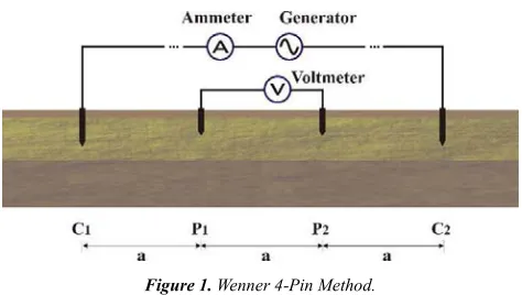
The design of electrical grounding systems can be a complex task but is essential to ensure people's safety and equipment integrity. Among various parameters which need to be considered during the design phase, the surrounding soil in which the grounding system is embedded is the most important one because it can affect significantly the grounding system performance. The soil structure model and its characteristics can be determined based on appropriate soil resistivity measurements. Therefore, the in-situ soil resistivity measurement is essential prior to any grounding design effort. The Wenner 4-Pin method of resistivity testing illustrated in Figure 1 is often used to provide the necessary field data for an accurate determination of the electrical soil structure model.
Figure 1. Wenner 4-Pin Method.
two potential electrodes (P1 and P2) placed along a straight line between the current-injection electrodes. The electrodes are all equally spaced. The spacing is increased from short distances of a fraction of a meter to distances on the order of the grounding system diagonal and more. Then, the so-called “apparent” resistivity is computed assuming an equivalent uniform soil model using the known expression 2πaV/I (in ohm-m), where “a” is the electrode (pin) spacing in meters,
V is the measured voltage in volts, and I is the injected current in amperes. In a uniform soil, the apparent resistivity is the actual resistivity of the soil. However, for a soil with multiple horizontal layers, the apparent resistivity measured at a certain pin spacing is a value representing the equivalent resistivity of entire stack of soil layers as seen by the electrodes at that particular spacing. Obviously, when the adjacent current and potential electrodes are very close to each other, resistivities of the shallow surface layers are dominant. When the electrodes are far apart, equivalent resistivities corresponding to the combined stack of soil layers at greater depths are reported, since the current can spread further downwards on its way from one outer electrode to the other. In fact, there is no simple relationship between the measured apparent resistivity and actual layer resistivities at depths comparable to the electrode spacing as some simple interpretation rules given in some documentations suggest.
The grounding system performance is heavily dependent on the soil structure and characteristics. When a fault occurs at a substation, a large amount of current is injected into the grounding system. This current flows throughout the grounding system, and leaks into the surrounding earth. A good understanding and accurate computation of the current distribution along the bare ground conductors and its dissipation in the surrounding earth are critical to predict the performance of a grounding system.
Many studies on soil resistivity measurements and grounding system designs have already been carried out and reported in several papers [1-7]. A number of interesting papers involving similar topics and their applications have been also published in recent years [8-13].
In this paper, however, one of the primary focuses is on current densities in the soil surrounding the current electrodes used to carry out the soil resistivity measurements. They have been explored in great detail in order to gain an intuitive understanding of what happens when the current is injected into one of the outer current electrodes and collected at the other one for different pin spacings. All analyses were carried out assuming three typical soil structure models, a uniform soil, a two layer soil model consisting of low-over-high resistivity layers, and a two-layer soil model consisting of high-over-low resistivity layers.
Another focus of this paper deals with the presence of nearby bare metallic structures, such as an existing nearby grounding system or any long bare metallic pipes (or its mitigation conductors) buried in the vicinity of the measurement traverse, which can seriously distort the measured soil resistivity values. The distortion of the current
density distribution in the soil due to such nearby metallic structures is displayed and discussed in order to provide a better overall understanding of the physical phenomenon that takes place in this case. A 100 ohm-m uniform soil is assumed in this study in order to concentrate solely on the influence of nearby metallic structures.
Finally, the paper focusses on the distribution of earth currents emanating from grounding systems in various soil structures. The computed results are shown graphically to illustrate the influence of soil structures on the performance of grounding systems.
Note that the uniform and two-layer soil models have been selected because they are the most representative ones that can be used in such a short technical paper. Other types of soils such as those involving finite volumes of heterogeneous materials can be studied in a similar way.
2. Methodology
To determine electrically equivalent layered soil structure models based on measured soil resistivity data, a standard inversion method for interpreting soil measurement data is employed. This computation method is based on numerical techniques usually called ‘Error Function Minimization’ [14-15]. It determines the parameters of the presumed soil model that will minimize the sum of the squares of the difference between the measured and computed apparent resistivities (Least-Square minimization algorithm). However, in this study, the direct soil resistivity computation process is used to emulate the resistivity measurement results that would be obtained in the field if the assumed soil model was present at the measurement site location. That is to say, a soil structure is selected first and a series of apparent resistivity values will then be computed up to sufficiently large pin spacings to reveal information regarding the deep soil characteristics based on the simulated soil resistivity test.
The analyses and computations of the soil resistivity measurements and grounding system performance are based on electromagnetic field theory [16], which is an extension to low frequencies of the moment method used in antenna theory. By solving Maxwell’s electromagnetic field equations, the method allows the computation of the current distribution as well as the charge or leakage current distribution in a network consisting of both aboveground and buried conductors with arbitrary orientations and which are bare or coated. It is an exact method that eliminates all of the assumptions mentioned in the conventional method. It accounts for attenuation, phase-shift and propagation effects in the electromagnetic fields when moving away from the current sources.
The distribution of the electric field and especially of the current density in the earth surrounding the electrodes and electrical grounding systems represent important physical parameters in the design of grounding systems and help better understand the effects of soil structures in grounding studies.
deduced from the computed electric field according to the following expression:
(1/
)
J
=
ρ ωε
+
j
⋅
E
(1)Where:
E: Electric field (V/m)
J: Current density (A/m2)
ρ: Soil resistivity (ohm-m)
ω: Angular frequency (rad/sec)
ε: Soil permittivity (F/m)
The current density vector components are complex quantities, with magnitude and phase. In this study, the magnitude of the resultant of the current density, i.e., the square root of
|
Jx
|
2+ |
Jy
|
2+ |
Jz
|
2, is computed and examined throughout the entire study.3. Simulations and Computation Results
3.1. Soil Resistivity Measurements
The purpose of the soil resistivity measurements related to the electrical grounding design is to assist in the determination of an appropriate soil model which should be used to evaluate the effect of the underlying soil characteristics on the performance of a grounding system. For grounding system studies, the soil is often typically modeled as a horizontally layered, isotropic electrical medium. Soil resistivity measurements are carried out according to the Wenner 4-Pin method [6-7] for the following three typical soil models:
(a).A 100 ohm-m uniform soil.
(b).A soil having a top layer resistivity of 100 ohm-m with a thickness of 5 m and a bottom layer resistivity of 5,000 ohm-m.
(c).A soil type consisting of a high resistivity layer of 5,000 ohm-m with a thickness of 5 m, over a low resistivity layer of 100 ohm-m.
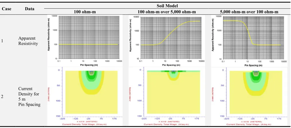
First, these three soil models have been predefined and the apparent resistivities have been computed using the direct soil resistivity computation process for a series of pin spacings starting at 0.1, 0.2, 0.3, 0.5, 0.7, 1, 2, 3, 5, 7, 10, … up to 5,000 m, i.e., very short and large pin spacings to adequately approach the resistivity of the top layer and that of the bottom layer in the case of a two layer soil model. The computed apparent resistivities have been plotted as shown in Case 1 of Table 1 as a function of the pin spacing used in the measurements.
Furthermore, the soil resistivity measurements in the three typical soil models, assuming a 1 A current injected in the current electrodes, have been simulated and analyzed using the electromagnetic field based software for a specific spacing of 5 m, 50 m, 500 m, and 1,000 m, respectively. Figure 2 shows an illustration of the measurement setup and of the soil current density distribution. The earth current densities have been computed over a vertical surface placed along the current and potential electrodes just beneath and perpendicular to the earth surface. Table 1 (Cases 2 to 5) shows the plots of the
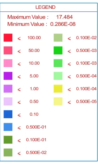
computed current density magnitude as a function of the pin spacing. Note that the current density is plotted in A/m2 and all of them have the same current density legend as shown in Figure 3.
Figure 2. An illustration of the measurement setup and of the soil current density distribution.
Figure 3. Current density plot legend.
The following observations can be made from these computation results:
(a).Different soil structures affect the apparent resistivity measurements in different ways as shown in the curves of Case 1 of Table 1.
(b).In a 100 ohm-m uniform soil, the apparent resistivity is always 100 ohm-m, as expected.
(c).In a soil having a 5 m thickness of 100 ohm-m top layer over a bottom layer of 5,000 ohm-m, the bottom layer resistivity is barely perceptible until the pin spacing reaches about 3 m. When the pin spacing is equal to the top layer thickness of 5 m, the apparent resistivity is 147 ohm-m. When the pin spacing is 10 m, the apparent resistivity is only 264 ohm-m. This definitely invalidates the commonly advocated notion
LEGEND
Maximum Value : 17.484
Minimum Value : 0.286E-08
100.00
50.00
10.00
5.00
1.00
0.50
0.10
0.500E-01
0.100E-01
0.500E-02
0.100E-02
0.500E-03
0.100E-03
0.500E-04
0.100E-04
that the soil resistivity at depth “a” is approximatively the same as the apparent resistivity at spacing “a”. Even when the pin spacing is equal to 50 m, the apparent resistivity is still 1,105 ohm-m far from the 5,000 ohm-m expected value. It is only when the pin spacing is about 1,000 m that the apparent resistivity reaches 4,617 ohm-m which is reasonably close to the expected bottom resistivity value.
(d).However, in a soil with a top 5 m thick high resistivity layer of 5,000 ohm-m over a low resistivity bottom layer of 100 ohm-m, when the pin spacing is 5 m, the measurement already suggests the presence of a low resistivity layer because the apparent resistivity drops to 3,473 ohm-m. At 50 m spacing, the measurement indicates an apparent resistivity value of 102.8 ohm-m which is essentially the expected bottom low resistivity layer.
These different behaviors are shown graphically by the current density plots displayed in Table 1 (Cases 2 to 5) in detail. The current density distribution is highly dependent on the soil structure.
In Case 2 of Table 1, the current electrodes are close together (spacing of 5 m). The resistivity near the surface of the earth is detected easily since most of the current flowing remains near the surface of the earth. This is particularly true for the 100 ohm-m over 5,000 ohm-m soil, most of the current passes through the top layer. However, in the 5,000 ohm-m over 100 ohm-m soil case, a large amount of the current penetrates rapidly into the low resistivity layer. That is why the apparent resistivity is 3,473 ohm-m at this short pin spacing.
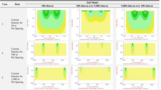
When the electrodes are spaced further apart, resistivities corresponding to soil layers at greater depths should be detected, since the current can spread further downwards on its way from one current electrode to the other. In Case 3 of Table 1, it is clear that at a spacing of 50 m, the 100 ohm-m
over 5,000 ohm-m soil case exhibits an apparent resistivity of 1,105 ohm-m though still far from the expected 5,000 ohm-m value. It is also obvious that a large amount of the current still passes through the top layer. On the other hand, in the 5,000 ohm-m over 100 ohm-m soil case, most of the current goes through the low resistivity bottom layer, that is why the apparent resistivity indicates a value of 102.8 ohm-m. This type of soil is quite sensitive to variations in soil resistivity with depth.
Cases 4 and 5 of Table 1 show that at a large spacing of 500 m and 1,000 m, the current for the 100 ohm-m over 5,000 ohm-m soil case is forced to circulate between the two current electrodes mainly through the bottom high resistivity layer despite the presence of a conductive top soil. The apparent resistivities are 4,038 ohm-m and 4,617 ohm-m, now getting close to the expected 5,000 ohm-m, though a small amount of current is still flowing in the top layer. Similarly, almost the entire current circulates between the pair of outer current electrodes through the bottom layer in the case of a 5,000 ohm-m over 100 ohm-m soil case. In this case, the apparent resistivity is almost equal to the expected value of 100 ohm-m.
This again emphasizes that it is certainly impossible to predict what pin spacing is required to determine the soil resistivity at a given depth. A comparison of the figures for the three types of soils suggests that the expectation or assumption that the measurement will provide the soil resistivity at the same depth as the pin spacing is a misleading argument.
The apparent resistivity reflects the response of all soil layers where the current must flow while travelling from one current electrode to reach the other current electrode as shown in Table 1. This is why the soil resistivity inversion algorithm is used to interpret measured data and determine an electrically equivalent soil structure.
Table 1. Apparent resistivities and current density distributions.
Case Data Soil Model
100 ohm-m 100 ohm-m over 5,000 ohm-m 5,000 ohm-m over 100 ohm-m
1 Apparent Resistivity
2
Case Data Soil Model
100 ohm-m 100 ohm-m over 5,000 ohm-m 5,000 ohm-m over 100 ohm-m
3
Current Density for 50 m Pin Spacing
4
Current Density for 500 m Pin Spacing
5
Current Density for 1,000 m Pin Spacing
3.2. Soil Resistivity Measurements in the Existence of Bare Metallic Structures Nearby
As can be seen from the above measurements, in general, apparent resistivity curves change smoothly and do not exhibit sudden changes although some resistivity variations may occur due to small local soil discontinuities, interference in the measurements such as stray currents in earth or inadequate sensitivity of the measuring equipment. However, the existence of bare metallic structures of significant length in the vicinity of measurement traverses may lower and distort measured resistivity values, such as extensive underground metallic water pipes or gas pipes equipped with mitigation wires, building foundations or grounding grids. These buried metallic structures will introduce alternative
electrical paths from one current electrode to another and result in false resistivity measurement predictions. In this part of the paper, the main objective is to study the influence of a buried metallic structure, i.e., a nearby existing grounding grid on soil resistivity measurements when the current pin spacing is varied from short to large values.
A series of soil resistivity simulation scenarios have been carried out with or without the presence of a nearby buried grounding grid. Figure 4 shows a plan view of the soil resistivity measurement electrode arrangement of the Wenner 4-Pin method and an adjacent 50 m x 100 m 16-mesh grounding grid buried at a depth of 0.5 m in a 100 ohm-m uniform soil. The measurement traverse runs parallel to the grid structure at a distance of 10 m from the edge of the grid.
Figure 5 shows the simulated measurement results along the traverse, i.e., apparent resistivities as a function of the current pin spacing (or total traverse spacing) starting from 0.9 m to 1,500 m, with and without the metallic structure, respectively. The resistivity curve corresponding to the case without the metallic structure is the red horizontal line; the “measured” soil resistivity for each spacing is 100 ohm-m regardless of the spacing, as expected. With the metallic structure, the yellow resistivity curve shows the measured “apparent” resistivities. This resistivity curve is no longer a straight horizontal line and the degree of deviation from the red horizontal line shows the intensity of the influence of the nearby metallic structure. In general, the measured “apparent” resistivities are quite close to the true soil resistivity of 100 ohm-m when the current pin spacing is either short or large compared to the structure size. The biggest distortion happens when the current pin spacing is about 100 m which is the length of the metallic structure.
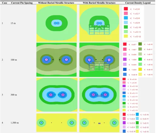
The current density distribution in the earth surrounding the current and potential electrodes has been analyzed and the results are shown in Table 2 in order to explain what happens to the resistivity measurements when there is a
buried metallic structure in the vicinity of the measurement traverse. Four representative scenarios for a current pin spacing of 15 m, 100 m, 300 m, and 1,500 m have been studied.
When the electrodes are close together, say, the current pin spacing is 15 m as shown in Case 1 of Table 2, the current density distribution around the electrode area (marked in blue), in the case with the metallic structure, exhibits the same pattern as in the case without the metallic structure, although a current density distortion within the area of the metallic structure can still be obversed. The reason is that the distance between the current electrodes and the metallic structure is 10 m and therefore, it is a relatively longer path for the current to take this rather long detour to travel between the current electrodes than travelling through soil where the area of the path available to the current increases as the square of the distance. Therefore, almost all the current will directly go through the soil and the measured apparent resistivity is 98.55 ohm-m which is very close to the true soil resistivity of 100 ohm-m. The buried structure clearly has little effect on the measurement.
Figure 5. Simulated apparent resistivity measurement results with or without a nearby buried metallic structure.
When the electrode spacing increases, the current electrodes are relatively far from each other and the soil current expanding out of each electrode is aware of the presence of a good conducting layer of meshed conductors on one side of the traverse that can serve as a favorable path. Indeed, the figures corresponding to a current pin spacing of 100 m in Case 2 of Table 2 clearly illustrate how the current density distributes in the soil throughout the entire area. In this case, the injected current at one of the electrodes is very close to the edge of the metallic structure; it is just 10 m compared to the distance to the other current electrode which
black dot) is shown as a dark yellow-green color, which is roughly two times larger than the one with a light grey-green color corresponding to the case of a nearby buried metallic
structure as indicated on the color legend. Note also that the current density within the structure area is much less than in other areas.
Table 2. Current density distributions with or without the existence of a buried metallic structure in a 100 ohm-m uniform soil.
Case Current Pin Spacing Without Buried Metallic Structure With Buried Metallic Structure Current Density Legend
1 15 m
2 100 m
3 300 m
4 1,500 m
On the other hand, when the current pin spacing becomes larger than the length of the metallic structure, say, 300 m as shown in Case 3 of Table 2, the current electrodes are far from the structure and therefore the influence from the structure is reduced gradually. However, the potential electrodes are still close to the structure and as a result, there is still less current density distribution between the potential electrodes and the measured apparent resistivity is 79.43 ohm-m as shown in Figure 5.
When the current pin spacing increases even further, the influence of the metallic structure becomes smaller and smaller. At the end, in the case that the current pin spacing reaches 1,500 m, the current density distribution is practically identical to the case without the metallic structure as shown in Case 4 of Table 2. Note that the figures are not at the same
scale with respect to each other.
3.3. Grounding System Performance
The electrical grounding system plays an extremely important role under fault conditions. Faults can damage equipment and facilities and lead to injuries, and even fatalities. When a large amount of short circuit current is injected into the grounding system, it flows throughout the grounding system and leaks into the surrounding earth from the bare ground conductors. The grounding system performance depends directly on the structure and characteristics of the soil. The design of grounding systems can be a complex task, since there are many variables, such as geometrical proportions of the grounding system, soil structure model, and ground conductor arrangement that can affect the behavior of the grounding system. Several articles [3-5] have studied the influence of those variables on the grounding system performance. The last part of this paper expands on this subject by focusing essentially on the current density distribution in the earth for different types of soil structures.
Figure 6 shows a plan view of three grounding grids with the following attributes.
(a).For Model (a), a 50 m x 100 m 36-mesh small grounding grid.
(b).For Model (b), a 100 m x 200 m large grid with the same number of meshes as for (a).
(c).For Model (c), a 100 m x 200 m large grid with 144 meshes and a mesh size equal to that of (a).
Figure 6. Plan view of the studied grounding grids.
All grids are buried at a depth of 0.5 m in the three typical soil models used in the previous study of soil resistivity measurements.
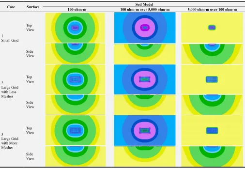
The leakage current densities for these three soil models have been computed and shown in Table 3. Note that current
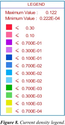
densities have been plotted on surfaces located at various depths in a 3D-spot fashion representing typical scans as shown in Figure 7. However, in Table 3, the current densities are displayed as two, 2D-spot surface plots, one corresponding to a horizontal surface located 1 m below the earth surface (top view) and the other one corresponding to a vertical surface across the center of the grid (side view) to easily see the distributions of the leakage current in more detail. The current densities are plotted in A/m2 and they all have the same legend as shown in Figure 8.
Figure 7. Current density distribution as a 3D-spot scan plot.
Figure 8. Current density legend.
The figures shown in Table 3 allow us to provide the following summary and conclusions:
(a).In the case of a 100 ohm-m uniform soil, the current density has a very similar pattern on the horizontal and vertical surfaces. The current spreads from the grounding system equally in all directions horizontally and vertically. The current moves away smoothly. However, this is no longer the case for the other two soil models. There are sudden changes when the soil resistivity varies.
(b).In the case of a 100 ohm-m over a 5,000 ohm-m soil, most of the current selects the less resistive top layer to
LEGEND
Maximum Value : 0.122 Minimum Value : 0.222E-04
0.30
0.10
0.700E-01
0.300E-01
0.100E-01
0.700E-02
0.300E-02
0.100E-02
0.700E-03
0.300E-03
0.100E-03
flow and much less current goes downwards. The current density in the top layer is considerably larger than the one for the uniform soil. Note that even when the grid is buried in a low resistivity layer, the current density inside the grid area is still the lowest while the current density around the perimeter conductors is the highest. This illustrates that the low frequency current tends to flow along conductors laterally first rather than downwards in the soil even when the grid is in the low resistivity layer.
(c).However, in the case of a 5,000 ohm-m over a 100 ohm-m soil, the current hardly moves laterally in the high resistive top layer and dissipates rapidly downwards to the bottom conductive layer.
(d).For the case of a large grid, the area size of the grounding system increases four times compared to the small grid, as shown in the figures in Cases 2 and 3 of
Table 3. Therefore, the current will distribute easily over a rather large area. However, it is interesting to see that the current density distribution varies at large distances in a similar way for both the small and large grids in all three different soil structures. This indicates that the current at a certain distance from the grounding system always spreads to remote earth roughly as hemispherical equipotential lines regardless of the shape of the grid.
(e).When the number of conductors increases, i.e., with more meshes, the overall current density distribution, as shown in the figures in Case 3 of Table 3, is not much different from the computation results shown in Case 2 of Table 3. It is clear that the number of grid conductors does not affect the current distribution in the earth significantly.
Table 3. Leakage current density distributions in the soil around the grounding grid (top and side views).
Case Surface Soil Model
100 ohm-m 100 ohm-m over 5,000 ohm-m 5,000 ohm-m over 100 ohm-m
1 Small Grid
Top View
Side View
2 Large Grid with Less Meshes
Top View
Side View
3 Large Grid with More Meshes
Top View
Side View
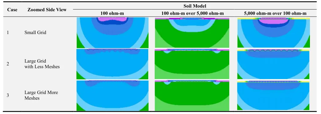
In order to look at more details of the current density at the areas that are close to the grounding grid, zoomed results on the vertical surface across the center of the grid have been plotted in Table 4. The following observations can be made:
(a).In the case of a 100 ohm-m uniform soil, the current tends to rise and fall from the center to the edge of the grid. The current density shows a lot of variation and the current density around the edge of the grid is very high. In particular, when the grid is large, the injected
(b).In the case of a 100 ohm-m over a 5,000 ohm-m soil model, the grid is in the low resistivity layer. As expected, the current density is much larger at the conductor end than in the middle. However, this phenomenon is quite significant in this type of soil due to the presence of a high resistivity layer beneath the low resistivity layer. The high resistivity layer prevents the current from going downwards. It is evident that the current flows away laterally in the top layer over a great distance.
(c).On the contrary, if the grid is in the high-resistivity layer as in the case of a 5,000 ohm-m over a 100 ohm-m soil, very little current flows in the top high resistivity layer away from the grid. The current has a tendency to go downwards quickly near the grid towards the bottom low resistivity soil and the variation of the leakage current density along each conductor is relatively small. That is why the current distribution is fairly uniform along almost all the conductors as shown in the figures.
Table 4. Leakage current density distributions in the soil around the grounding grid (zoomed side view).
Case Zoomed Side View Soil Model
100 ohm-m 100 ohm-m over 5,000 ohm-m 5,000 ohm-m over 100 ohm-m
1 Small Grid
2 Large Grid with Less Meshes
3 Large Grid More Meshes
4. Conclusion
The design of electrical grounding systems is crucial to ensure people's safety and equipment integrity. The performance of the grounding system is critically dependent on the characteristics of the local soil surrounding the grounding system.
This paper focused on three main aspects of grounding design, namely soil resistivity measurements in various soil model structures, effects of nearby buried metallic structures on such measurements and finally, performance of grounding grids in layered soils. The paper illustrates graphically the results for the three important aspects of grounding design while clarifying and invalidating some concepts and assumptions that are still prevalent among some electrical designers nowadays.
In the first part, soil resistivity measurements using the Wenner method in three typical, but different soil structure models, were examined by exploring the distribution of earth current density in the soil surrounding the current injection electrodes. The results show that the apparent resistivity measured at one specific spacing cannot be used to conclude what the real resistivity is at a certain depth. The computed results are illustrated using appropriate plots to understand better the influence of soil structure and characteristics on the current penetration across the soil layers. In the second part of the paper, a detailed study on the influence of nearby buried grounding systems on soil resistivity measurements
was carried out. The study shows that when a measurement traverse runs parallel to a nearby large metallic structure, a significant error can be introduced. Caution should be taken to minimize the influence of buried metallic structures on soil resistivity measurements. Finally, the last part of the paper focused on the behavior and performance of grounding systems with various grid sizes and mesh sizes in three typical soil structures. All scenarios have been studied to better illustrate and understand the effects of soil structures on grounding.
All computed results are summarized in appropriate tables and figures which should provide helpful visual clues and useful information when planning soil resistivity measurements and designing electrical grounding systems.
Acknowledgements
The authors wish to thank Dr. Simon Fortin and Mr. Robert Southey of SES for their constructive comments and assistance.
References
[1] F. P. Dawalibi and D. Mukhedkar, "Parametric Analysis of Grounding Grids," IEEE Transactions on PAS Vol. 98, No. 5, Sept.-Oct. 1979, pp. 1659-1668.
[3] F. P. Dawalibi and N. Barbeito, "Measurements and Computations of the Performance of Grounding Systems Buried in Multilayer Soils," IEEE Transactions on PWRD, Vol. 6, No. 4, October 1991, pp. 1483-1490.
[4] F. P. Dawalibi, J. Ma, and R. D. Southey, "Behaviour of Grounding Systems in Multilayer Soils: a Parametric Analysis," IEEE Transactions on Power Delivery, Vol. 9, No. 1, January 1994, pp. 334-342.
[5] H. Lee et al., “Efficient Grounding Designs in Layered Soils,” IEEE Trans. Power Del., vol. 13, No. 3, pp. 745–751, Jul. 1998. [6] J. Ma and F. P. Dawalibi, "Study of Influence of buried Metallic Structures on Soil Resistivity Measurements," IEEE Transactions on Power Delivery, Vol. 13, No. 2, April 1998, pp. 356-363.
[7] R. D. Southey and F. P. Dawalibi, “Improving the Reliability of Power Systems with More Accurate Grounding System Resistance Estimates,” in Proc. Int. Conf. Power Syst. Technol., Oct. 2002, vol. 1, pp. 98–105.
[8] H. Zhao, S. Fortin and F. P. Dawalibi, “Analysis of Grounding Systems Including Freely Oriented Plates of Arbitrary Shape in Multilayer Soils,” IEEE Transactions on Industry Applications, Vol. 51, No. 6, November/December 2015, pp. 5189-5197. [9] S. Fortin, N. Mitskevitch and F. P. Dawalibi, “Analysis of
Grounding Systems in Horizontal Multilayer Soils Containing Finite Heterogeneities,” IEEE Transactions on Industry Applications, Vol. 51, No. 6, November/December 2015, pp. 5095-5100.
[10] J. Liu, F. P. Dawalibi and B. F. Majerowicz, “Gas Insulated
Substation Grounding System Design Using the Electromagnetic Field Method,” The 5th China International Conference on Electricity Distribution (CICED), Shanghai China, September 5-6, 2012.
[11] X. Wu, V. Simha, and R. J. Wellman, “Strategies for designing a large EHV station ground grid with drastically different soil structures,” Transmission and Distribution Conference and Exposition (T&D), 2016 IEEE/PES. Dallas, TX, USA, 3-5 May 2016.
[12] A. Ackerman, P. K. Sen, and C. Oertli, “Designing Safe and Reliable Grounding in AC Substations with Poor Soil Resistivity: An Interpretation of IEEE Std. 80,” IEEE Transactions on Industry Applications, Vol. 49, Issue. 4, July-Aug. 2013, pp. 1883-1889.
[13] M. Nassereddine, J. Rizk, M. Nagrial, and A. Hellany, “Substation and Transmission Lines Earthing System Design under Substation Fault,” Electric Power Components and Systems, Volume 43, 2015 - Issue 18, September 2015, pp. 2010-2018.
[14] F. P. Dawalibi and F. Donoso, "Integrated Analysis Software for Grounding, EMF, and EMI," IEEE Computer Applications in Power, Vol. 6, No. 2, April 1993, pp. 19-24.
[15] R. S. Baishiki, C. K. Osterberg, and F. P. Dawalibi, "Earth Resistivity Measurements Using Cylindrical Electrodes at Short Spacings," IEEE Transactions on Power Delivery, Vol. 2, No. 1, January 1987, pp. 64-71.