Transmission Wheeling Pricing in Embedded Cost Using
Modified Amp-Mile and MVA Utility Factor Methods
Gaurav Jain
1,*, Dheeraj Kumar Palwalia
2, Anuprita Mishra
31,2Department of Electrical Engineering, Rajasthan Technical University, Kota, India
3Department of Electrical Engineering, Technocrats Institute of Technology, Bhopal, India
Received 11 January 2019; received in revised from 27 February 2019; accepted 28 March 2019
Abstract
Transmission wheeling pricing is one of the decisive aspects of present open access electricity market. Various
methods are available for transmission; however, no method is proved to diverse operating conditions of the power
system. These methods are not able to quantify the full recovery of embedded cost. All the variables i.e. remaining
charges, used circuit capacity are not counted in the existing methods. This paper explicates two methods, Modified
Amp-Mile method, and MVA Utility Factor method, to recover the embedded cost. Modified Amp-Mile method is a
customized form of existing Amp-Mile method. In the MVA Utility Factor method, cost allocation is based on
Marginal Participation (MP). It evaluates the cost, using sensitivity analysis of network power. The proposed
methods are tested on an IEEE 6-bus system and further verified on Hadoti region real 37-bus system. All the results
are presented in Full Recovery Model (FRM) and Partial Recovery Model (PRM).
Keywords: transmission wheeling pricing, embedded cost recovery, open access, power system economics
1.
Introduction
In reference to the Indian electrical network, Power Plant and electrical utilities are connected to the same transmission
network. A nodal point is required to decide transmission pricing by independent power producers and electrical utilities both.
The action of one buyer creates an effect on other participants; hence practical cost allocation becomes difficult to investigate
[1]. However, transmission cost allocation is a complicated issue in deregulated power system [2]. In past years, different
methods for allocation of transmission cost in electric networks are proposed by researchers. Capacity usage related to each
transaction is calculated for all transmission lines by applying existing methods i.e. Average Participation method, Marginal
Participation method, Distribution Factors, Equivalent Bilateral Exchange method, Z-bus method, and Cooperative Game
Theory.
In open access, electricity market allotment of embedded cost is one of the important aspects [3]. Each utility has to find a
solution with the characteristics of its transmission system and degree of deregulation adopted. Various methods are employed
at all operational conditions of diverse power systems to obtain such a solution. No technique is capable of evaluating the entire
embedded cost. Any usage-based cost allocation method must contain three features, i.e. accurate algorithms for transmission
usage evaluation, equitable allocation rules and full recovery of embedded cost. Based on the above features, cost allocation
signifies to identify cost causer for incurring these costs. To determine the causer may be complicated because the non-linear
nature of power flow equalities causes difficulty to nature of power flow equations [4].
Existing methodologies used for transmission wheeling pricing are classified into rolled-in methods and
usage-basedmethods. The rolled-in methods do not provide price signals that are cost reflective and are subdivided into two
methods, i.e. Postage Stamp Method and Contract Path Method. In Postage Stamp Method, electric utilities allocate the fixed
cost among its users having firm contracts [5]. Whereas, in Contract Path Method [6] managed power would be confined to an
artificially specified path through the transmission system. On the other hand, usage-based methods require power flow
execution of the transmission system and divided into various sub-categories, i.e. MW-Mile, Modulus, MVA-Mile, and
Amp-Mile methods. MW-Mile methodology [7] is the pricing strategy for the recovery of fixed transmission costs on the basis
of actual power flow of the transmission network. In the Modulus method, all mediators have to pay for the actual capacity use
and additional reserve [8]. MVA-Miles method is an augmented version of MW-miles; it takes into account the range of the
use of network due to their active and reactive power injection/drawn [9]. Whereas, Amp-Mile method is based on the current
flow in the system.
Marginal Participation (MP) methods dominate tracing flow methods as there is no electrical principle behind the tracing
flow [10]. It is implemented where tracing flow is significantly less. It allocates transmission charges to either generators or
demand nodes. The allocation between generators and demands is decided exogenously, therefore it distorts the vocational
signal. It assigns power flow sensitivity in each line due to power injection at each bus and the network usage cost. Sensitivities
or utility factors evaluated as per MP are used to predict the changes in losses, voltages and different branch flow due to change
in loads and generations [11]. These sensitivities capture the effects of unbalanced network parameters, load and generator
locations. In marginal participation methods, the Amp-Mile method is enough to attain the aim for the transmission network.
Even though it has some limitation, i.e. it cannot be implemented on EHV networks and cannot allocate entire embedded cost.
Hence, additional charges are required to be imposed on agents. In practice, the Extent of Use (EU) is never 100% of the
circuit’s capacity. Therefore, the grid looks underutilized and lastly service cost based on the network usage will be smaller
than embedded cost. Other costs are incurred through supplementary charges [12].
In transmission wheeling, there are many challenges occur to find out proper coat allocation. Some challenge is to
promote the efficiency of the day-to-day operation of the bulk power market. To resolve the problem of signal locational
advantages for investment in generation and demand. To increase the investment in the transmission system for saving
customer cost in the energy market. Recover the costs of existing transmission assets, which has been investment by the
transmission company. In transmission pricing, incremental cost is directly available from economic dispatch. These pricing
methods are well suited for rapid on line costing, but limited to presenting economic effects on the wheeling utility’s
production cost and total system losses. The main focus is to find ways and means to generate and inject more competition,
thereby forcing the conventional monopolistic power market to a competitive market. The transmission of open access has
been introduced into the electric power supply industry to alter the traditionally monopolized market. It is desired that
transmission prices and payment do not disturb decisions for new generation investment, for generator and for consumer
demand. At same time charging must be achieved in a simple and fair form, realistic and adequate for real-time application as
well as transparent enough to be politically acceptable. In wheeling,methodology compute a high priority problem due to
growth in transmission facilities, cost differentials between utility companies, and dramatic growth in non-utility generation
capacity.
The Modified Amp method in the full recovery model and MVA utility factor method in full/partial recovery model is
analyzed in this paper. Cost comparison analysis of the different method is show benefits of Modified Amp method in
transmission pricing. The embedded cost allocations using a different method at different percentage loading are evaluated. A
real 37-bus system and IEEE 6-bus system network is used in the case study to prove efficiency and applicability of the
proposed method. In this paper, the nonlinearity of sensitivity indices of Modified Amp method and MVA utility factor has
2.
Wheeling Pricing Methodologies
The pricing methodology adopted by each utility is depending on the characteristic of the transmission or distribution
network. Therefore, a particular pricing methodology cannot be applied for all conditions as each methodology has its specific
characteristics. Deregulated environment reduces the tariff for consumers and improves the efficiency for power suppliers in
the long run. Transmission pricing has been categorized on the basis of their operating principles i.e. Marginal/Incremental
cost-based pricing [13], Embedded cost-based pricing [14], and combination of Embedded with Incremental cost-based
pricing [15].
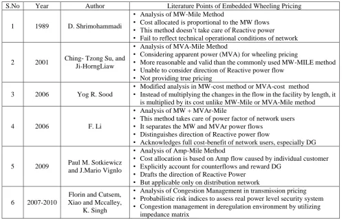
Table 1 Literature methodology in embedded wheeling pricing from past to present
S.No Year Author Literature Points of Embedded Wheeling Pricing
1 1989 D. Shrimohammadi
• Analysis of MW-Mile Method
• Cost allocated is proportional to the MW flows
• This method doesn’t take care of Reactive power
• Fail to reflect technical operational conditions of network
2 2001 Ching- Tzong Su, and
Ji-HorngLiaw
• Analysis of MVA-Mile Method
• Considering apparent power (MVA) for wheeling pricing
• More reasonable and valid than the commonly used MW-MILE method
• Unable to consider direction of Reactive power flow
• Not providing true pricing
3 2006 Yog R. Sood
• Modified analysis in MW-cost method or MVA-cost method
• Instead of multiplying the changes in the flow in the facility by length, it is multiplied by its cost unlike MW-Mile or MVA-Mile method
4 2006 F. Li
• Analysis of MW + MVAr-Mile
• This method takes care of power factor of network users
• It separates the MW and MVAr power flows
• Distinguishes direction of Reactive power flow
• Acknowledges full cost-benefit of network users, especially DG
5 2009 Paul M. Sotkiewicz
and J.Mario Vignlo
• Analysis of Amp-Mile Method
• Cost allocation is based on Amp flow caused by individual customer
• Explicitly account for counterflows and reward DG
• Drafts the direction of Reactive Power
• But applicable only on distribution network
6 2007-2010
Florin and Cutsem, Xiao and Mccalley,
K. Singh
• Analysis of Congestion Management in transmission pricing
• Probabilistic risk indices to assess real power level security system
• Congestion management in deregulation environment by utilizing impedance matrix
2.1. Marginal/ incremental cost-based pricing methods
Marginal pricing or marginal wheeling rates are also called an extension of the spot-pricing theory. Spot pricing is a
method for pricing electricity that maximizes the economic efficiency of the power system [16]. It is difficult to estimate
transmission pricing using marginal cost based pricing method as the income would not be sufficient for financing the
investment. However, a theory of social benefit, which maximizes real-time price of real and reactive powers, is considered
[17]. It flattens the peak power demand and fills the valley of demand. The allocation of transmission payments among
different agents depends upon the total energy consumed. An algorithm for optimal pricing includes transmission cost beside
generation cost in electricity supply. The report of optimal pricing calculation has to be sent to all the participants. The
marginal cost could be minimized with the inclusion of FACTS devices in an overloaded transmission system. FACTS devices
can change power flows by using system parameters. Using spot pricing and marginal cost theories active and reactive power
transition costs is calculated while voltage-dependent load models were observed [18].
Incremental cost methodologies are defined in two parts as short run and long run cost. Short run marginal/incremental
cost or spot pricing is economic. It has some bidding to power transmission systems such as entire transmission costs not
recovered, the charges acquired exceedingly volatile, rationale for transmission charges and the transmission system is
data with uncertainties. It is difficult to obtain convincing prices as many non-deterministic factors are involved [19]. All
system costs (existing transmission system, operation, and expansion) are allocated among the system users in proportion to
their EU (Extent of Use) of the transmission resources. The charge for basic transmission service is usually the component of
overall transmission service charges.
2.2. Embedded cost-based pricing methods
Embedded cost is defined as the revenue required paying for all existing or any new facilities added to the power system
during the contract for transmission service. In general form adequate remuneration of transmission systems and easy to
implement. The embedded cost methods allocate the total system cost among the transmission customers, based on Extent of
Use (EU) rule. In embedded methods, all system costs (existing transmission system, operation, and expansion) are allocated
among the system users in proportion to their Extent of Use (EU) of the transmission resources. They can be classified as
rolled-in methods and usage-based methods. The main shortcoming of the rolled-in methods is ignorance of actual system
operation. As a result, they are likely to send incorrect economic signals to transmission customers. But this problem has
overcome by usage-based methods as it evaluates EU in the framework of either load flow or optimal power flow. Embedded
costs methods are used by the utilities to allocate existing transmission facilities to the transmission wheeling transaction.
Table 1 represents the literature survey of embedded wheeling pricing. This table easily describes embedded wheeling cost
strategy in electricity market from past to present stage.
2.2.1. Active power flow based methods
The capacity of transmission network used for a transaction is a function of the magnitude of electric power, transmission
lines length, and facilities involved in the active power transaction. Capacity value provides an equitable means of allocating
the cost of transmission facilities among users of the firm transmission service. It takes full account of current generation cost
and capacities as well as the transmission of the demand in space and time. The mw-mile method is used to evaluate the
transmission pricing leads to the effective recovery of all embedded costs. It includes an analysis of relative reliability
contributions of each generator to the unscheduled transmission capacity in a circuit. All transmission users are liable to wages
the actual use of capacity and transmission reserves. In practice, it is improper for those who make limited usage of the
network.
2.2.2. Real power flow based methods
J. Bialek proposed a tracing flow method for evaluating the flow of electricity through power networks [20]. It allows
quantification of active or reactive power flows from a particular source to a specific load, the contribution from each generator,
power load flow and losses in a line. Kirschen’s method is based on the solution of a series of load flows. It calculates the
contribution of the generator to the loads, line flows and transmission pricing. J. Bialek proposed another tracing flow
methodology is known as Unifying Tracing-based methodology of transmission pricing for inter-system trades. It is easy,
transparent and fast. It can also deal effectively with circular flows.
An up-gradation of MW-Mile method was introduced in the year 2001. The upgrade technique is called a MVA-Mile
method which reflects the EU of transmission facilities in the system. It enforces to power flow and considers apparent power.
It is reasonable and valid in comparison to the commonly used MW-mile method, but big wheeling charge may pick up the
total generation cost. Monetary Path method is also based on tracing flow concept, which proposes an even measurement for
transmission usages by active and reactive powers. Reactive power allocation method determines real and imaginary currents
to handle the system losses and loop flow. The traces from current sources to current sinks are then converted to power
contributions. MVA method is economic to resolve difficult reactive power pricing and costing issues. All the methods are
2.3. Composite embedded and marginal cost-based pricing methods
TThis methodology includes both the existing system cost and marginal costs of transmission transactions to evaluate the
collective transmission pricing part by embedded cost and marginal pricing method. The marginal cost based pricing is used to
transmission price services. It requires supplement revenue generation as a pricing scheme is not able to care financially to the
transmission service providers. This approach discriminates between operating and embedded costs. It develops separate
methods in respect of each of these components. The capacity utilized as well as consistency benefits derived by different users
for investment recovery payout of charges for investment recovery are considered. It also includes marginal pricing approach
to the recovery of operating cost. It is a simple novel method used for topological analysis of power flows based transmission
supplement charge allocation in the network. Its result is positive in counter-flow contributions from all the users. Revenue of
transmission company divided into marginal cost and supplementary charges. The marginal cost is evaluated by FRM model to
estimate the total transmission cost (cost allocation and remaining charges). In supplementary charges, the cost is evaluated by
PRM model. Whereas, locational charges and post stamp charges method is used to estimate the supplementary charges. Both
methods are used to evaluate remaining charges in supplementary cost. The supplementary charges are allocated in real power
as well as reactive power load through MW-Mile, MVA-Mile method. This charge for usage of a separate transmission asset is
divided into a locational and non-locational component. Wheeling charging strategy and unused capacity of the asset are
shown in Fig. 1.
Fig. 1 Wheeling charging strategy
2.4. Amp-mile method
The Amp-Mile method is an embedded cost allocation method for the medium voltage distribution network. It is based on
the Extent of Use (EU) for circuits is measured in terms of the contribution of each customer to the current flow i.e. the power
to current distribution factors (APIDFlkt& RPIDFlkt), at any instant of time. It is the least control of system stability (steady state
and transient) in the distribution system. Current capacity increases up to the thermal limit. So current flows may attribute
network customers, therefore method is acknowledged as “Amp-mile” or “I-mile” methodology [1]. Thus different Extent of
Use (EU) is found out using current distribution factors and used to accomplish allocation of cost. Unambiguously accounts for
flow direction to provide better long-term price signals and to alleviate potential constraints [20]. Steps to allocate embedded
t t
t lk k
lk t
l APIDF PL AEoUL
AI
(1)
t t
t lk k
lk t
l
APIDF PG
AEoUG
AI
(2)
t t
t lk k
lk t
l
RPIDF QL REoUL
AI
(3)
t t
t lk k
lk t
l RPIDF QG REoUG
AI
(4)
where, 𝐴𝐸𝑜𝑈𝐿𝑡𝑙𝑘 is Active EU of circuit 𝑙 at time 𝑡 due to demand at 𝑘𝑡ℎ bus, 𝐴𝐸𝑜𝑈𝐺𝑙𝑘𝑡 is Active EU of circuit 𝑙 at time 𝑡 due to generation at 𝑘𝑡ℎ bus, 𝑅𝐸𝑜𝑈𝐿𝑡𝑙𝑘 is Reactive EU of circuit 𝑙 at time 𝑡 due to demand at 𝑘𝑡ℎ bus, 𝑅𝐸𝑜𝑈𝐺𝑙𝑘𝑡 is Reactive EU of circuit 𝑙 at time 𝑡 due to generation at 𝑘𝑡ℎ Bus, 𝐴𝑃𝐼𝐷𝐹𝑙𝑘𝑡 is Active power to current distribution factor of circuit 𝑙 at time 𝑡 due to demand at 𝑘𝑡ℎ bus, 𝑅𝑃𝐼𝐷𝐹𝑙𝑘𝑡 is Active power to current distribution factor of circuit 𝑙 at time 𝑡 due to demand at 𝑘𝑡ℎ bus.
Various methods are not able to quantify the EU of a transmission network for both active and reactive power flows. The
Amp-Mile method became the base of the research. Limitations of Amp-Mile method have been identified through numerical
value. Based on these corrections Modified Amp-Mile method is proposed. It recommends applicability on EHV networks by
putting more prominence on stability limits. A step ahead introduced a new usage-based cost allocation technique- MVA
Utility Factor method with two models: Full Recovery and Partial Recovery Model. It carries the advantages of Modified
Amp-Mile method. It is based on marginal participation; therefore obtained utility factors are prone to the choice of slack bus.
Therefore distinct slack bus notion has been proposed to allocate the embedded cost of EHV networks. Distinct slack bus
notion is different from dispersed slack bus concept. The intermediate stages of nonlinear sensitivities are found using
modified NR based load flow. The relationship between flow and power injection/withdrawal is nonlinear. The novel
sensitivity patterns could assist ISO to forecast day-ahead transmission. In full recovery model total EU for all the lines
remains unity under all loading conditions.
3.
Proposed Methodology
The amp-mile method has some limitations. When the system has fully loaded this method do not recover the full
embedded cost. It is relevant only on radial networks since currents are comparative to the thermal capacity of the distribution
network (high R/X ratio). It is stated that circuit currents are an approximately linear function of active and reactive power at
the bus in a radial network. In Amp-Mile a reconciliation factor is needed to find EU factors for a given line sum to unity. It
confers only two types of sensitivities (Eq.(5)) in the form of Transmission factors CUPF (Current Utility Active Factor) and
CUQF (Current Utility Reactive Factor). The common transmission factor for demand/generation transmutation at the same
bus with a difference of sign.
l dk l gk
I
P
I
P
(5)l dk l gk
I
Q
I
Q
(6)where, 𝐼𝑙is the absolute value of the current through circuit l, 𝑃𝑑𝑘 is the active power withdrawal due to demand at 𝑘𝑡ℎ bus, 𝑃𝑔𝑘
is the active power withdrawal due to generation at 𝑘𝑡ℎ bus, 𝑄𝑑𝑘is the reactive power withdrawal due to demand at 𝑘𝑡ℎ bus,
3.1. Modified amp-mile method
The modified Amp-Mile method identifies the nonlinear or linear nature of sensitivities depending on location and
topological conditions. Its charges allocation has not been stable at variable load levels and different period of time. It indicates
that the current sensitivity indices CUPFtlk and CUQFtlk are exhibiting nonlinear nature with respect to active and reactive
powers (injection/withdrawal) at a bus of EHV network. Modified NR based load flow is used to find current sensitivity
indices. In the modified Amp-Mile method, reconciliation factor is not required to furnish the total EU for a given line equal to
unity. It selects new distinct slack bus perception to resolve the load flow values. Entire embedded cost of EHV networks is
allocated by using non-linear sensitivities and new distinct slack bus notion.
If a system has large chances of increase in load and generation on the same bus, comparisons could be made between
∂Il⁄∂Pdk and ∂Il⁄∂Pgk. Therefore, current sensitivity indices are expressed as t
ldk l dk
CUPF I P (7)
t
lgk l gk
CUPF I P (8)
t
ldk l dk
CUQF I Q (9)
t
lgk l gk
CUQF I Q (10)
where, 𝐶𝑈𝑃𝐹𝑙𝑑𝑘𝑡 is Current utility active factor of 𝑙𝑡ℎline w.r.t.𝑘𝑡ℎ demand bus at 𝑡𝑡ℎinstant, 𝐶𝑈𝑃𝐹𝑙𝑔𝑘𝑡 is Current utility active factor of 𝑙𝑡ℎline w.r.t.𝑘𝑡ℎ generator bus at 𝑡𝑡ℎ instant, 𝐶𝑈𝑄𝐹𝑙𝑑𝑘𝑡 is Current utility reactive factor of 𝑙𝑡ℎline w.r.t.𝑘𝑡ℎ demand bus at 𝑡𝑡ℎinstant, 𝐶𝑈𝑄𝐹𝑙𝑔𝑘𝑡 is Current utility reactive factor of 𝑙𝑡ℎline w.r.t.𝑘𝑡ℎ generator bus at 𝑡𝑡ℎinstant.
The applicability of the modified Amp-Mile method is on EHV networks, by putting more prominence on stability limits,
instead of thermal capability. In Eq. (5), there should be dissimilarity between CUPFlkt and CUQFlkt for load/generation given in Eqs. (7-10). The expressions of dissimilar EU’s are
where, 𝐴𝐸𝑈𝐷𝑙𝑘𝑡 is Active extent of use by 𝑘𝑡ℎ bus demand for 𝑙𝑡ℎ line at 𝑡𝑡ℎ instant, 𝐴𝐸𝑈𝐺𝑙𝑘𝑡 is Active extent of use by 𝑘𝑡ℎ
bus generation for 𝑙𝑡ℎ line at 𝑡𝑡ℎ instant, 𝑅𝐸𝑈𝐷𝑙𝑘𝑡 is Reactive extent of use by 𝑘𝑡ℎ bus demand for 𝑙𝑡ℎ line at 𝑡𝑡ℎ instant,
𝑅𝐸𝑈𝐺𝑙𝑘𝑡 is Reactive extent of use by 𝑘𝑡ℎ bus generation for 𝑙𝑡ℎ line at 𝑡𝑡ℎ instant, 𝑃𝑑𝑘𝑡 is Active demand on 𝑘𝑡ℎ bus at 𝑡𝑡ℎ
instant, 𝑃𝑔𝑘𝑡 is Active generation on 𝑘𝑡ℎ bus at 𝑡𝑡ℎinstant, 𝑄𝑑𝑘𝑡 is Reactive demand on 𝑘𝑡ℎ bus at 𝑡𝑡ℎ instant, 𝑄𝑔𝑘𝑡 is Reactive
generation on 𝑘𝑡ℎ bus at 𝑡𝑡ℎinstant, 𝐼𝑙𝑡 is Absolute current in 𝑙𝑡ℎ line at 𝑡𝑡ℎinstant.
The reconstruction of the algorithm to evaluate CUPFlkt and CUQFlkt inherently attributes the efficacy of slack bus power. It provides true sensitivities, re-establishing and offered a close approximation of circuit currents.
The expression of the absolute value of Ilt will turn to
Substitute used circuit cost at tth instant (UCClt) equal to unity to find the allocation of embedded cost. Consequently adapted circuit cost at tthinstant (ACClt) would be equal to CClt and therefore the relation of locational charges change as given below
? )
t t t t t t
lk ldk dk l l dk dk l
AEUD CUPF P I I P P I (11)
? )
t t t t t t
lk lgk gk l l gk gk l
AEUG CUPF P I I P P I (12)
? )
t t t t t t
lk ldk dk l l dk dk l
REUD CUQF Q I I Q Q I (13)
? )
t t t t t t
lk lgk gk l l gk gk l
REUG CUQF Q I I Q Q I (14)
1 nbus
t t t t t t t t t
l ldk dk lgk gk ldk dk lgk gk
k
I CUPF P CUPF P CUQF Q CUQF Q
where, 𝐴𝐿𝑡𝑘is Active Locational charge due to active demand on 𝑘𝑡ℎ bus at 𝑡𝑡ℎinstant, 𝐴𝐺𝑘𝑡 is Active Locational charge due to active generation on 𝑘𝑡ℎ bus at𝑡𝑡ℎinstant, 𝑅𝐿𝑡𝑘 is Reactive Locational charge due to reactive demand on 𝑘𝑡ℎ bus at 𝑡𝑡ℎ instant,
𝑅𝐺𝑘𝑡 is Reactive Locational charge due to reactive generation on 𝑘𝑡ℎ bus at 𝑡𝑡ℎinstant, 𝐶𝐶𝑙𝑡 is a level cost for each hour.
The expression of remaining circuit charges (𝑅𝐶𝐶𝑡) are
So the total cost of the modified Amp-Mile method in the full recovery model is
The modified Amp-Mile method increases allocation equivalent to full recovery model in proportion to assorted EU’s.
The EU’s of all circuits would be unity under all loading conditions and no need to calculate remaining (supplementary or
non-vocational) charges. Therefore, keeping UCC equal to unity and evaluate transmission charges plus capacity charges
simultaneously. Transmission network participants have to pay for used/unused capacity in proportion to their EU. It is
justified by the need for system meeting reliability, stability and security criteria for all customer.
3.2. MVA utility factor method
The MVA Utility Factor method allocates the entire embedded cost of transmission networks. It carries the advantages of
previously discussed modified Amp-Mile method. The non-linear patterns of MVA utility factors have been furnished and
distinct slack bus notion has been promoted to allocate the embedded cost of power networks. It provides better promises for
payments to counterflow creators and gives assurance for prudent implementation.
In the proposed technique individual participant’s impact on the system is recognized through MVA flow caused by them.
Therefore, a method is called an MVA Utility Factor method. It is a significant method because no question arises in relation to
current limits for the reason that MVA flows can be increased under specified constraints of the power network. It wiped out
limits of the modified Amp-Mile method and exploits load flow and derives non-linear sensitivities (MVAUF).
This illustrates a true understanding of the network and causes a fair allocation. In MVA utility factor method, unequal
sensitivities at a bus having active/reactive generation and load are represented as [21].
where, 𝑀𝑉𝐴𝑃𝑈𝐹𝑙𝑑𝑘𝑡 is MVA utility active factor of 𝑙𝑡ℎline w.r.t.𝑘𝑡ℎ bus demand at 𝑡𝑡ℎinstant, 𝑀𝑉𝐴𝑃𝑈𝐹𝑙𝑔𝑘𝑡 is MVA utility active factor of 𝑙𝑡ℎ line w.r.t.𝑘𝑡ℎ bus generator at 𝑡𝑡ℎinstant, 𝑀𝑉𝐴𝑄𝑈𝐹𝑙𝑑𝑘𝑡 is MVA utility reactive factor of 𝑙𝑡ℎline w.r.t.𝑘𝑡ℎ bus demand at 𝑡𝑡ℎ instant, 𝑀𝑉𝐴𝑄𝑈𝐹𝑙𝑔𝑘𝑡 is MVA utility reactive factor of 𝑙𝑡ℎline w.r.t.𝑘𝑡ℎbus generator at 𝑡𝑡ℎinstant.
1
line
n
t t t
k lk l
l
AL AEUD CC
(16)
1
line
n
t t t
k lk l
l
AG AEUG CC
(17)
1
line
n
t t t
k lk l
l
RL REUD CC
(18)
1
line
n
t t t
k lk l
l
RG REUG CC
(19)
1
[ ] 0
line
n
t t t
l l
l
RCC CC CC
(20)
?
tk kt tk ktTotal Cost
AL
AG
RL
RG
(21)t t
lgk ldk
MVAPUF MVAPUF (22)
t t
lgk ldk
The transmission network though EHV network does not follow the same for some of the generator buses using load flow.
It obtains either equal or unequal sensitivities at generator buses in EHV networks. Therefore, Eqs. (22-23) does not reflect true
operating conditions. Many cost allocation methodologies suggested following load flow to avoid unequal sensitivities. It
established four different utility factors corresponding to generator buses in EHV networks irrespective of equal or unequal
sensitivities. MVA flow of a line can be expressed using utility factors of Eqs. (24-27) are
where, 𝑀𝑉𝐴𝑙𝑡 is the absolute value of MVA through circuit l, 𝑃𝑑𝑘𝑡 is the active power withdrawal due to demand at 𝑘𝑡ℎ bus at
𝑡𝑡ℎ instant, 𝑃
𝑔𝑘𝑡 is the active power withdrawal due to generation at 𝑘𝑡ℎ bus at 𝑡𝑡ℎ instant, 𝑄𝑑𝑘𝑡 is the reactive power withdrawal
due to demand at 𝑘𝑡ℎ bus at 𝑡𝑡ℎ instant, 𝑄𝑔𝑘𝑡 is the reactive power withdrawal due to generation at 𝑘𝑡ℎ bus at 𝑡𝑡ℎ instant. Formulation of MVAUF’s is evaluated using modified NR based load flow. Thus attributes the effect of slack bus power. These buses are self-regulating and bounds for each of the generators. It maintains a constant voltage at buses; consequently,
no change in line flow occurs due to change in a reactive generation. Expression of Absolute MVA in lthline at tthinstant (MVAtl) are
The MVAUF’s from Eqs. (24-27) are employed for the evaluation of EOU by each participant, equations given as:
It is concluded that total EU due to all participants is unity even though the system is not fully loaded. This methodology
is utilized to develop two types of allocation models; Partial Recovery Model (PRM) and Full Recovery Model (FRM).
3.2.1. Partial recovery model (PRM)
In this modal, a part of the embedded cost is allocated on the basis of electricity usage and remaining charges are imposed
on the participants. The two types of charges are;
PUBC: Charge allocated to participants based on the real usage of the network.
RC: This portion of allocation reflects a charge to recover the cost of the unused network capacity. It is revealing the
security issue of the power system and has to be imposed on all participants. Expressions of PUBC and RC are:
t t t
ldk l dk
MVAPUF MVA P (24)
t t t
lgk l gk
MVAPUF MVA P (25)
t t t
ldk l dk
MVAQUF MVA Q (26)
t t t
lgk l gk
MVAQUF MVA Q (27)
1 nbus
t t t t t t t t t
l ldk dk lgk gk ldk dk lgk gk
k
MVA MVAPUF P MVAPUF P MVAQUF Q MVAQUF Q
(28)
t t t t
lk ldk dk l
AEUD MVAPUF P MVA (29)
t t t t
lk lgk gk l
AEUG MVAPUF P MVA (30)
t t t t
lk ldk dk l
REUD MVAQUF Q MVA (31)
t t t t
lk lgk gk l REUG MVAQUF Q MVA
Both models by a utility depend on its transmission system and extent of deregulation espoused. (32)
1 nline
t t t
dk lk l
l
PUBCP AEUD ACC
where, 𝑃𝑈𝐵𝐶𝑃𝑑𝑘𝑡 is Partial recovery usage-based charges for active demand on 𝑘𝑡ℎ bus at 𝑡𝑡ℎ instant, 𝑃𝑈𝐵𝐶𝑃𝑔𝑘𝑡 is Partial recovery usage-based charges for active generation on 𝑘𝑡ℎ bus at 𝑡𝑡ℎ instant, 𝑃𝑈𝐵𝐶𝑄𝑑𝑘𝑡 is Partial recovery usage-based charges for reactive demand on 𝑘𝑡ℎ bus at 𝑡𝑡ℎ instant, 𝑃𝑈𝐵𝐶𝑄𝑔𝑘𝑡 is Partial recovery usage-based charges for reactive generation on 𝑘𝑡ℎbus at 𝑡𝑡ℎ instant.
Let 𝐶𝐶𝑙𝑡 is levelized hourly cost of 𝑙𝑡ℎcircuit and annual circuit cost will be𝐶𝐶𝑙𝑡× 8760.Then corresponding adapted circuit cost 𝐴𝐶𝐶𝑙𝑡 at 𝑡𝑡ℎ instant is
where𝑈𝐶𝐶𝑙𝑡 is the used circuit capacity of line 𝑙 for time 𝑡, and defined by
where 𝐶𝐴𝑃𝑙 is MVA capacity of the line. The Remaining Charge (RC) express as
3.2.2. Full recovery model (FRM)
Accomplishes total recovery of embedded cost by substituting 𝑈𝐶𝐶𝑙𝑡 unity in Eq. (37); consequently, 𝐴𝐶𝐶𝑙𝑡 would be equal to 𝐶𝐶𝑙𝑡. Expressions of FUBC are:
where 𝐹𝑈𝐵𝐶𝑃𝑑𝑘𝑡 is Full recovery usage-based charges for active demand on 𝑘𝑡ℎbus at 𝑡𝑡ℎinstant, 𝐹𝑈𝐵𝐶𝑃𝑔𝑘𝑡 is Full recovery usage-based charges for active generation on 𝑘𝑡ℎbus at 𝑡𝑡ℎinstant, 𝐹𝑈𝐵𝐶𝑄𝑑𝑘𝑡 is Full recovery usage-based charges for reactive demand on 𝑘𝑡ℎbus at 𝑡𝑡ℎInstant, 𝐹𝑈𝐵𝐶𝑄𝑔𝑘𝑡 is Full recovery usage-based charges for reactive generation on 𝑘𝑡ℎbus at 𝑡𝑡ℎinstant.
In FRM, the Eq. (38) for Remaining Charges can be modified accordingly and expressed as:
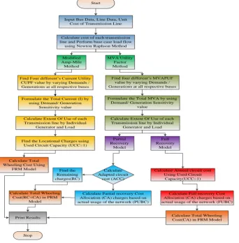
Using an analysis of both methodologies a flow chart is shown in Fig. 2. Data input and newton raphson analysis is the
same in both methods. Current utility factor logic has been used in mod amp mile method similarly;
1 nline
t t t
gk lk l l
PUBCP AEUG ACC
(34)
1 nline
t t t
dk lk l
l
PUBCQ REUD ACC
(35)
1 nline
t t t
gk lk l
l
PUBCQ REUD ACC
(36)
t t t
l l l
ACC UCC CC (37)
/
t t
l l l
UCC MVA CAP (38)
1 nline
t t t
l l
l
RC CC ACC
(39)
1 nline
t t t
dk lk l
l
FUBCP AEUD CC
(40)
1 nline
t t t
gk lk l
l
FUBCP AEUG CC
(41)
1 nline
t t t
dk lk l
l
FUBCQ REUD CC
(42)
1 nline
t t t
gk lk l
l
FUBCQ REUG CC
(43)
1
0 nline
t t t
l l
l
RC CC CC
MVA sensitivity analysis has been used to calculate the MVA utility factor method. Used circuit capacity (UCC=1) unity
value is used to calculate annual circuit cost which is defined FRM wheeling value in both methods. MVA utility factor PRM
model represent adapted circuit cost to evaluate Cost Allocation (CA) and Remaining Charges (RC) in the network.
Start
Input Bus Data, Line Data, Unit Cost of Transmission Line
Calculate cost of each transmission line and Perform base case load flow
using Newton Raphson Method
Modified Amp-Mile Method MVA Utility Factor Method
Find four different’s MVAPUF value by varying Demands / Generations at all respective buses
Formulate the Total MVA by using Demand/ Generation Sensitivity
value
Calculate Extent Of Use of each Transmission line by Individual
Generator and Load Find Four different’s Current Utility
CUPF value by varying Demands / Generations at all respective buses
Partial Recovery Model Full Recovery Model
Calculate Annual circuit cost Using Used Circuit
Capacity(UCC=1)
Calculate Partial recovery Cost Allocation (CA) charges based on actual usage of the network (PUBC)
Calculate Adapted circuit cost (ACC) Find the Remaining charges(RC)
Calculate Total Wheeling Cost(RC+CA) in PRM
Model
Stop Print Results
Calculate Full recovery Cost Allocation (CA) charges based on actual usage of the network (FUBC)
Calculate Total Wheeling Cost(CA) in FRM Model Formulate the Total Current (I) by
using Demand/ Generation Sensitivity value
Calculate Extent Of Use of each Transmission line by Individual
Generator and Load
Find the Locational Charges using Used Circuit Capacity (UCC=1)
Calculate Total Wheeling Cost Using
FRM Model
Fig. 2 Flow chart of mod amp-mile and MVA utility factor methods
4.
Case Study and Results
The proposed methodologies have to be employed on some real-time system or IEEE standard bus system to prove its
efficiency and reliability. In this paper, a real-time 37 bus system and one IEEE standard 6 bus system is used as a case study
and respective results are discussed. In the case study, Modified Amp-Mile method is applied using full recovery modal,
whereas, MVA utility factor method is applied using both modals i.e. full and partial recovery modal. Single line diagram of
real-time 37 bus system is shown in Fig.3. The system has 2 generation bus and 48 transmission corridors at 220 kV and 132
kV voltage level. The generation capacity of 1300 MW is assumed as base load condition and total load connected on the
system is 911 MW. It is assumed in this analysis that load customer would pay 100% of the transmission cost of services to the
transmission utility. The annual revenue requirement of transmission facility is 843.56 Crs-INR. The embedded cost to be
allocated is assumed proportional to the length of individual transmission lines in Rupee/hr. The comprehensive detail and
various parameters of the 37 bus system are given in Table 2. Data of total load connected is collected of each feeder Whereas,
bus data represent the bus voltage, active/reactive value of generated power and total load connected in different buses. In line
data values represent the load connection information for every node , value of the impedance in each line of the system and
Fig. 3 North Indian Real Test System (Power Map of 37 bus Hadoti Region)
Table 2 Cost of generation and load (Rupee / hr.) for real 37 bus system
Bus data of 37-bus Transmission System Line Data of 37-bus Transmission System Bus
no. Bus voltage Power generated Load
Node
Connection Impedance(p.u.)
Line Charging
Magnitude Angle P Q P Q From To R X (p.u.) B/2
(pu) (deg) (MW) (MVAr) (MW) (MVAr) 1 2 0.00024 0.001275 0
1 1 0 1300 0 0 0 1 5 0.0056 0.02975 0
2 1.01 0 0 0 0 0 1 3 0.00896 0.0476 0
3 1.02 0 0 0 0 0 2 6 0.00672 0.0357 0
4 1 0 0 0 0 0 2 15 0.0306397 0.0794612 0
5 1.02 0 0 0 0 0 2 21 0.0132314 0.0343144 0
6 1 0 0 0 0 0 2 22 0.01001 0.02596 0
7 1 0 0 0 18 7.1 2 23 0.0206388 0.0535248 0
8 0.98 0 0 0 28 10.17 2 7 0.0295022 0.0765112 0
9 0.99 0 0 0 10 3.3 2 18 0.03822 0.09912 0
10 0.98 0 0 0 20 7.27 2 36 0.000455 0.00118 0
11 0.98 0 0 0 20 7.24 3 4 0.00456384 0.0242454 0
12 0.99 0 0 0 26 8.52 3 8 0.0352625 0.09145 0
13 1 0 0 0 20 6.57 3 17 0.00864045 0.0224082 0
14 1.03 0 0 0 14 4.61 3 35 0.000455 0.00118 0
15 0.98 0 0 0 40 11.68 4 28 0.01630064 0.0865972 0
16 0.98 0 0 0 20 5.82 4 9 0.0186732 0.0484272 0
17 1 0 0 0 35 12.69 4 12 0.05027295 0.1303782 0
18 1 0 0 0 25 9.87 4 13 0.03069976 0.079617 0
19 0.98 0 0 0 30 7.53 4 17 0.0142506 0.0369576 0
20 0.98 0 0 0 40 10.04 4 19 0.03586401 0.09301 0
21 1 0 0 0 42 16.6 4 34 0.000455 0.00118 0
22 1 0 0 0 80 31.64 5 15 0.00728 0.01888 0
23 0.99 0 0 0 85 33.6 6 31 0.00738848 0.0392513 0
24 0.98 0 0 0 29 7.28 6 21 0.0219583 0.0569468 0
25 1 0 0 0 20 4.98 6 23 0.0219583 0.0569468 0
26 0.99 0 0 0 35 8.76 6 24 0.0281372 0.0729712 0
27 1 0 0 0 30 7.53 6 37 0.000455 0.00118 0
28 1 0 300 0 0 0 8 9 0.175266 0.0454536 0
29 1.02 0 0 0 0 0 8 10 0.0219947 0.0570412 0
30 0.98 0 0 0 35 8.76 8 11 0.053235 0.13806 0
31 1.02 0 0 0 0 0 12 14 0.0344799 0.0894204 0
32 0.98 0 0 0 25 6.25 15 16 0.02548 0.06608 0
33 1 0 0 0 35 8.76 18 20 0.02002 0.05192 0
34 1 0 0 0 42 13.8 19 20 0.02928289 0.0759424 0
35 1 0 0 0 25 9.09 20 24 0.0228046 0.0591416 0
36 1 0 0 0 50 19.75 20 25 0.0154245 0.040002 0
37 1 0 0 0 32 8.02 20 30 0.0250068 0.0648528 0
Table 2 Cost of generation and load (Rupee / hr.) for real 37 bus system (continued)
24 31 0.0153517 0.0398132 0 25 29 0.0336245 0.087202 0 26 29 0.0104923 0.0272108 0 27 29 0.0173628 0.0450288 0 28 29 0.00668 0.0354875 0 29 31 0.0079472 0.0422195 0 29 33 0.000455 0.00118 0 30 32 0.042345868 0.1098533 0 30 31 0.00637 0.01652 0
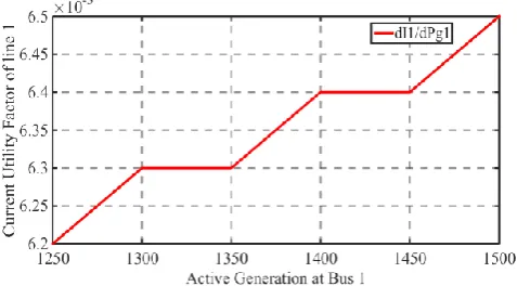
4.1. Non-linear nature of sensitivity indices
Load flow is being used either for transmission network or EHV network to obtain equal sensitivities and unequal
sensitivities. An inequality in curve nature is depending upon magnitude. Whereas, magnitude depending on the choice of
slack bus, location of generator bus and transmission line.During load flow, any bus can be assigned as a slack bus. Load flow
neglects longitudinal resistance, the conductance of network elements, reactive power flow and considers all voltages equal to
unity. In result, the magnitude of injection/withdrawal variation at any generation bus directly influences loss compensation.
Lines connected to the slack bus would have different flow variations and lines away from the slack bus would have less
impact. The equivalent feature is narrated in Rudnick’s method [4]. The evaluation of the total impact of injection/withdrawal
of electrical power is independent for each bus. Amount of allocation depends on currency cost impact. At bus payments are
made by the utility to participants, reflecting the proposed technique identifies the negative EU due to reactive demand.
(a) Non Linear CUPFt1g1 for 37 bus system (b) Non Linear CUPFt21d10 for 37 bus system
(c) Non Linear CUPFt9d7 for 37 bus system (d) Non Linear CUQFt16d9 for 37 bus system
Fig. 4 Nonlinear CUPF curve of generation and load in 37 bus system
Fig. 4(a-d) shows the nonlinear sensitivity behavior curves for modified Amp-Mile method. The real or reactive MVA
sensitivities would not be identical at generator buses. It exhibits nonlinear nature of sensitivities depending upon location and
topological conditions. Fig. 4(a-d) shows the nonlinear sensitivity curves for MVA utility factor method. The estimation and
non-linear sensitivities. Patterns of sensitivities assessed for variation of P and Q at all buses for different loading by employing
load flow analysis. The sensitivity patterns have many advantages for a deregulated market.
(a) Provide price signals for the future generation/demand expansion.
(b) Forecast transmission pricing, if used along with EU values.
(c) Congestion anticipation and used to manage congestion either by curtailing the demand.
(d) Assist ISO to carry out the day ahead scheduling in the deregulated electricity market.
(a) Non Linear MVAPUFt16g1 for 37 bus system (b) Non Linear CUPFt21d10 for 37 bus system
(c) Non-Linear CUPFt9d7 for 37 bus system (d) Non-Linear CUQFt16d9 for 37 bus system
Fig. 5 Nonlinear MVAPUF curve of generation and load in 37 bus system
4.2. Cost allocation andcost curve
Evaluate the total cost in Rupee/hr by using mathematical operation of both the proposed methods. For IEEE 6 bus
standard system, comparison of the proposed model (Partial Recovery Model and Full Recovery Model) has been brought
down. Cost Allocated (CA), Remaining Charge (RC), and Embedded Cost (EC) are to be compared for at all buses by
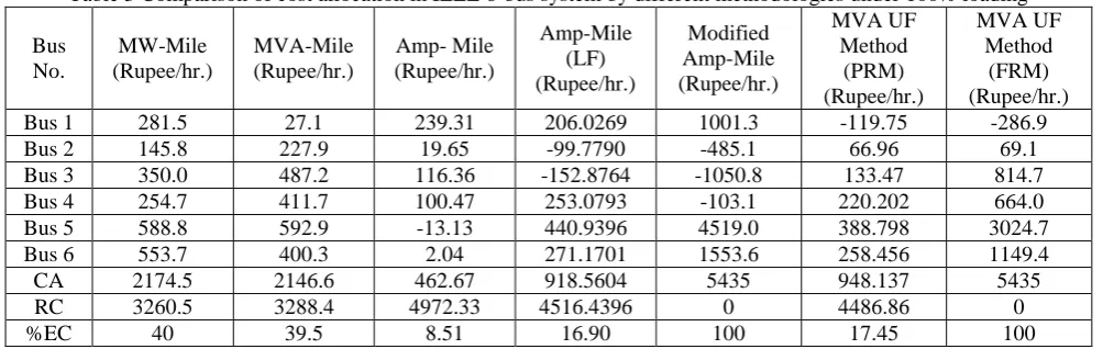
employing different techniques. Table 3 shows the comparison of all the costs including RC and % EC of each bus.
By observing Table 3, execution of the MVA Utility Factor method causes a striking reduction in cost allocated to Bus 1
(slack bus), as positive payments by all other methods are turning to negative payments. Likewise, cost allocation is negative to
Bus 5 load and positive to the first generator in Amp-Mile method. It shows reflecting payments are made by transmission
utility to load and recovered from generators, which seems unjustified. This problem gets resolved through proposed MVA
Utility Factor method using either Partial Recovery model or Full Recovery model. Realization of proposed modified
Amp-Mile and MVA utility factor method proved to be superior over MW-Mile method, MVA-Mile method, and Amp-Mile
method. Its advantages like FRM of EHV networks contrasting Amp-Mile tackles reactive power unlike MW-Mile and
anticipates the direction of reactive power not like MVA-Mile. The cost to be allocated in modified Amp-Mile and MVA
utility factor method is assumed proportional to the length of transmission lines in Rupee/hr. In IEEE 6 bus system the total
cost evaluated in modified Amp-Mile and MVA utility factor methods in FRM condition is 5435 Rupee/hr. Whereas, In PRM
as cost allocated or zero amount as remaining charges in modified Amp-Mile and MVA Utility Factor method (FRM only). All
the other existing methods along with proposed MVA Utility Factor method (PRM) have a significant amount as remaining
charges. Hence, these methods do not allocate 100% embedded cost. The negative sign represent the return cost given by the
transmission company.
Table 3 Comparison of cost allocation in IEEE 6-bus system by different methodologies under 100% loading
Bus No.
MW-Mile (Rupee/hr.)
MVA-Mile (Rupee/hr.)
Amp- Mile (Rupee/hr.)
Amp-Mile (LF) (Rupee/hr.)
Modified Amp-Mile (Rupee/hr.)
MVA UF Method
(PRM) (Rupee/hr.)
MVA UF Method
(FRM) (Rupee/hr.)
Bus 1 281.5 27.1 239.31 206.0269 1001.3 -119.75 -286.9
Bus 2 145.8 227.9 19.65 -99.7790 -485.1 66.96 69.1
Bus 3 350.0 487.2 116.36 -152.8764 -1050.8 133.47 814.7
Bus 4 254.7 411.7 100.47 253.0793 -103.1 220.202 664.0
Bus 5 588.8 592.9 -13.13 440.9396 4519.0 388.798 3024.7
Bus 6 553.7 400.3 2.04 271.1701 1553.6 258.456 1149.4
CA 2174.5 2146.6 462.67 918.5604 5435 948.137 5435
RC 3260.5 3288.4 4972.33 4516.4396 0 4486.86 0
%EC 40 39.5 8.51 16.90 100 17.45 100
The locational and remaining charges allocation at different loadings has been estimated using diverse cost allocation
techniques. The evaluated cost allocated under the different percentage of Base Case (BC) loading conditions by different
methodologies is shown in Table 4. It has been observed that the cost allocation by employing Modified Amp-Mile method is
constant for all loading conditions. The percentage embedded cost is 100% are zero remaining charges are allocated in
modified Amp-Mile method irrespective of loading of the system. Hence, Modified Amp-Mile method is seen to be the most
excellent method for full recovery modal only, under each loading condition. Before evaluating the cost of the system, check
the degree of congestion at BC loading specifically for overloading, to keep the system secured.
Table 4 Embedded cost (Rupee/hr.) allocation in IEEE 6-bus system by different methods at different % loading Methods
Loadings 50% 75% 100% 125% 150%
MW-Mile 1488.6 1860.6 2174.5 3045.2 2980.0
Rem. Cost (MW) 3946.4 3574.4 3260.5 2389.8 2455
MVA-Mile 1288.8 1672.6 2146.6 4100.3 3371.6
Rem. cost (MVA) 4146.2 3762.4 3288.4 1334.7 2063.4
Amp-Mile (Base) 190.153 252.19 462.67 713.08 1107.6
Rem. Cost(I-Mile) 5244.8 5182.8 4972.33 4721.9 4327.4
Amp-Mile(LF) 882.8 847.6 918.56 1098.9 1264.1
Rem. Cost (Amp-Mile(LF)) 4552.2 4587.4 4516.44 4336.1 4170.9
Mod. Amp-Mile 5435.0 5435.0 5435.0 5435.0 5435.0
Rem. cost (Mod. Amp-Mile) 0 0 0 0 0
Any generator bus can be assigned as a slack bus for estimation of cost and to find CUF’s. Consider another generator bus
as the new slack bus and then cost allocation associated withthe new slack bus has been evaluated. All the costs, CA, RC, and
%EC has been evaluated for the new slack bus by employing different methodologies and compare the results as shown in
Table 5.
The utilities have a different region with significant local load and generation. The injection in a given region may cause
an increment in the circuit flows all around the country. Resulting tariffs are sometimes nonspontaneous with generators that
are close to load centers in a given region receives high tariffs. Therefore the currency cost impact of the different slack bus by
implementing distinct slack bus notion is used. Results for depiction on the IEEE 6 bus system are given in Table 4 at Base
Case (BC) loading.
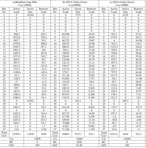
Embedded cost is evaluated using modified Amp-Mile and MVA utility factor method for 37 bus system in a similar
Table 6(c). Whereas, PRM costs are shown in Table 4 (b) for MVA utility factor method only. Table 4 illustrates the generation
and load cost allocates at different buses for active and reactive power. The allocations by FRM at all busses are given in Table
6(a) and (c).
Table 5 Cost impact (Rupee/ hr) of the new slack bus at 100% base
Bus No. Amp-Mile (LF) Slack Bus -Bus1
Mod. Amp-Mile Slack Bus-Bus1
Amp-Mile(LF) Slack Bus –Bus 2
Mod. Amp-Mile Slack Bus –Bus 2
Bus 1 206.0269 1001.3 60.4148 360.1
Bus 2 -99.7790 -485.1 234.5645 1042.3
Bus 3 -152.8764 -1050.8 -87.6418 -2317.3
Bus 4 253.0793 -103.1 144.6832 -272.8
Bus 5 440.9396 4519.0 344.1372 4615.5
Bus 6 271.1701 1553.6 157.5987 2007.2
CA 918.5604 5435 853.7567 5435
RC 4516.4396 0 3727.4866 0
%EC 16.90 100 15.71 100
It has been observed that the payments are made by transmission utility to participants due to the counter flow of power. In
37 bus system, the total cost evaluated is 13699 Rupee /hr. in Modified Amp-Mile and MVA Utility Factor methods (FRM
condition only.) Whereas, In PRM condition, MVA utility factor allocated cost is12699 Rupee/Hr. In Table 6 real 37 bus
system FRM model are recover the full Allocation Cost (AC) in both the technique. This result analysis represents the
beneficial effect of the proposed work. The remaining charges are also calculated by the postage stamp method. Compare the
remaining charges cost in IEEE 6 bus and real 37 bus system. The low remaining charges in real 37 bus test system are showing
the good stability in pricingwheeling market. That is more beneficial for generators and consumer in the electrical energy
market (real-world strategies).
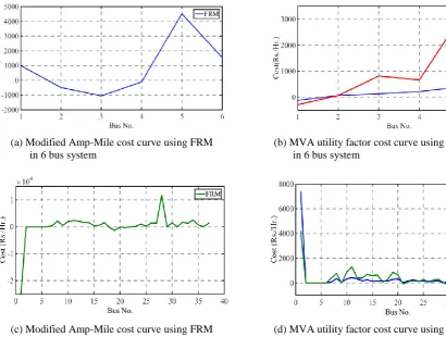
(a) Modified Amp-Mile cost curve using FRM in 6 bus system
(b) MVA utility factor cost curve using PRM & FRM in 6 bus system
(c) Modified Amp-Mile cost curve using FRM in 37 bus system
(d) MVA utility factor cost curve using PRM & FRM in 37 bus system
Table 6 Cost of generation and load (Rupee / hr.) for real 37 bus system
(a)Modified Amp-Mile Cost (FRM)
(b) MVA Utility Factor Cost(PRM)
(c) MVA Utility Factor Cost (FRM)
Bus Active Active Reactive Bus Active Active Reactive Bus Active Active Reactive
No. Load Gen Load No. Load Gen Load No. Load Gen Load
1 0 -24761 0 1 0 7371 0 1 0 4155 0
2 0 0 0 2 0 0 0 2 0 0 0
3 0 0 0 3 0 0 0 3 0 0 0
4 0 0 0 4 0 0 0 4 0 0 0
5 0 0 0 5 0 0 0 5 0 0 0
6 0 0 0 6 0 0 0 6 0 0 0
7 306.5 0 102.1 7 69.996 0 10.63 7 352.1 0 53.52
8 1832.8 0 339.4 8 311.17 0 48.64 8 674.9 0 103.3
9 495.7 0 39.2 9 48.233 0 5.087 9 -6 0 -8.438
10 1570.8 0 308.8 10 285.67 0 42.96 10 763.2 0 110.2
11 1929.3 0 397.1 11 380.01 0 56.01 11 1153.3 0 164.8
12 1892.2 0 236 12 294.2 0 37.56 12 359.9 0 45.51
13 1459.2 0 181.8 13 160.03 0 18.95 13 358.8 0 38.64
14 1372.9 0 210.7 14 226.81 0 27.36 14 632.1 0 70.26
15 404.9 0 46.7 15 124.06 0 10.79 15 529.7 0 46.38
16 507.9 0 70.7 16 132.13 0 11.11 16 597.2 0 50.32
17 1413.5 0 157.8 17 159.57 0 29.63 17 56.7 0 22.32
18 -272.2 0 -31.5 18 127.24 0 17.02 18 237.7 0 37.08
19 -1100.4 0 -165.4 19 270.3 0 22.51 19 797.9 0 64.66
20 -52.1 0 -51.6 20 311.26 0 22.83 20 617.9 0 54.82
21 -326.2 0 -17.3 21 34.024 0 3.751 21 -56.1 0 -11.68
22 37 0 -11.5 22 132.65 0 34.6 22 59.7 0 28.67
23 209.8 0 -74.8 23 203.7 0 51.1 23 142.4 0 48.96
24 997 0 74.2 24 160.32 0 9.624 24 121.6 0 1.48
25 202.8 0 -14.9 25 122.56 0 9.513 25 238.3 0 19.57
26 1384.6 0 49.9 26 95.874 0 8.288 26 130.1 0 7.14
27 1290.4 0 54.1 27 110.22 0 8.769 27 221.2 0 12.6
28 0 11822 0 28 0 162.1 0 28 0 289.1 0
29 0 0 0 29 0 0 0 29 0 0 0
30 1441.2 0 54.3 30 161.64 0 8.622 30 -119.7 0 -35.27
31 0 0 0 31 0 0 0 31 0 0 0
32 1623.4 0 154.4 32 267.23 0 16.05 32 457.1 0 10.19
33 1252.2 0 45.4 33 47.783 0 5.438 33 -1.6 0 -0.64
34 2253.4 0 253.3 34 189.05 0 21.16 34 -38.8 0 -4.04
35 656.5 0 93.1 35 79.808 0 15.34 35 30.3 0 11.71
36 1.4 0 1.1 36 4.022 0 0.582 36 -4.9 0 -0.71
37 14.6 0 1336 37 71.246 0 1.159 37 14.6 0 -9
Total
22799.1 -12939 3839 Total 4580.8 7533.1 555.1 Total 8321.6 4445 933.3
Cost Cost Cost
CA 13699 CA 12669 CA 13699
RC 0 RC 1030 RC 0
%EC 100 %EC 92.48 %EC 100
Fig. 6 show cost curve nature of PRM and FRM for MVA utility factor method, whereas, only FRM for Modified
Amp-Mile method. Fig. 6(a) and (b) are drawn by using data of Table 3, whereas, Fig. 6(c) and (d) are drawn by using data of
Table 6.
The price instability significantly affects the results of both the proposed methods. Fundamentally Modified Amp-Mile
and MVA Utility method shows different characteristics with the fluctuations in demand. Therefore, transmission price and
demand are the essential characteristics for the estimation of cost allocation. Variations in the curve are depending on the
magnitude. Proposed methodologies are fair, accurate and feasible for estimation of cost if the cost allocation is prepared as per
the demand. MVA utility factor technique is simple in application and provides price signals. The dissimilarity in the cost
curve shown in Fig. 6(b) is due to PRM allocation is 17.45% of the entire embedded cost and remaining 82.55% allocate
through supplementary charges, whereas, FRM allocated 100% embedded cost for both the methods. Similarly, in Fig. 6(d),
FRM allocates 100% embedded cost, but PRM allocates 92.48% of the entire embedded cost. In PRM energies due to the
Capacity (UCC), which is always less than unity. Hence, the quality of decrement may cause a disparity in the sign of
allocation of both the model as shown in Fig. 6.
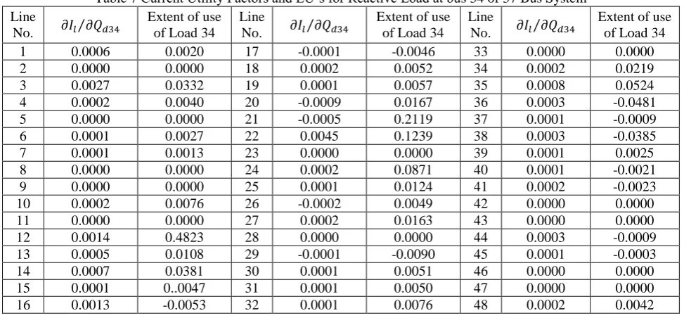
In results, current utility factor and EU’s are also used in both techniques. Implementation of this technique proved to be
superior over MW-Mile and MVA-mile method along with full recovery. Table 7 shows the current utility factor and EU’s of
reactive power, reflecting the direction of reactive power. Through cost allocation by these existing methods appear to be
uniform but due to mentioned limitations well through-out to be inexcusable.
Table 7 Current Utility Factors and EU’s for Reactive Load at bus 34 of 37 Bus System Line
No. 𝜕𝐼𝑙⁄𝜕𝑄𝑑34
Extent of use of Load 34
Line
No. 𝜕𝐼𝑙⁄𝜕𝑄𝑑34
Extent of use of Load 34
Line
No. 𝜕𝐼𝑙⁄𝜕𝑄𝑑34
Extent of use of Load 34
1 0.0006 0.0020 17 -0.0001 -0.0046 33 0.0000 0.0000
2 0.0000 0.0000 18 0.0002 0.0052 34 0.0002 0.0219
3 0.0027 0.0332 19 0.0001 0.0057 35 0.0008 0.0524
4 0.0002 0.0040 20 -0.0009 0.0167 36 0.0003 -0.0481
5 0.0000 0.0000 21 -0.0005 0.2119 37 0.0001 -0.0009
6 0.0001 0.0027 22 0.0045 0.1239 38 0.0003 -0.0385
7 0.0001 0.0013 23 0.0000 0.0000 39 0.0001 0.0025
8 0.0000 0.0000 24 0.0002 0.0871 40 0.0001 -0.0021
9 0.0000 0.0000 25 0.0001 0.0124 41 0.0002 -0.0023
10 0.0002 0.0076 26 -0.0002 0.0049 42 0.0000 0.0000
11 0.0000 0.0000 27 0.0002 0.0163 43 0.0000 0.0000
12 0.0014 0.4823 28 0.0000 0.0000 44 0.0003 -0.0009
13 0.0005 0.0108 29 -0.0001 -0.0090 45 0.0001 -0.0003
14 0.0007 0.0381 30 0.0001 0.0051 46 0.0000 0.0000
15 0.0001 0..0047 31 0.0001 0.0050 47 0.0000 0.0000
16 0.0013 -0.0053 32 0.0001 0.0076 48 0.0002 0.0042
By evaluating the non-linear curve, cost allocation, remaining charges, current utility factor, and EU’s. Some important
factors are originated. Both methods recover 100 embedded costs in a comparison to the existing method. When compare the
IEEE 6-bus and 37-bus system in MVAPUF PRM model. The cost allocation value is 17.45% and 92.48 % respectively.
Therefore 37-bus practical system cost allocation is more suitable as a comparison to the IEEE system. So both methodologies
are reliable for the practical transmission network. The non-linear nature of curve is used to assessing true portrayal of
operating condition load flow has followed to develop fair allocation. The sensitivity patterns can help ISO to forecast
day-ahead transmission cost as well as plan for day-ahead setting up of open access electricity market.
5.
Conclusions
In open access, electricity market allotment of embedded cost is one of the momentous facets. The two methodologies for
allocation of the embedded cost of transmission network i.e. Modified Amp-Mile method and MVA Utility Factor method
with two models: Full Recovery and Partial Recovery, has been employed in this paper.
The proposed method exploits marginal participation in the load flow framework. The nonlinear sensitivities for the current
utility of active and reactive powers have been discussed in this paper. The nonlinear sensitivities in power networks which
are used to anticipate congestion and transmission price forecasting.
Fair cost allocation in the presence of nonlinear sensitivities is solved by employing proposed Modified Amp-Mile
methodology. It is implemented on prices and sensitivities with respect to injections/withdrawals of power in the modern
electricity market.
MVA Utility Method in two different modals i.e. FRM and PRM is employed for estimation of fair cost allocation.
Non-linear sensitivities and distinct slack bus notion are promoted to allocate the partial or entire embedded cost of the
Results show that the wheeling charges for Modified Amp-Mile and MVA Utility Factor method have approached more
close solutions to MW-Mile, MVA-Mile and Amp-Mile methods for the 6-bus and 37-bus test system.
Comparison of other existing techniques for IEEE 6-bus system confirms the effectiveness of the proposed method. The
impact of loading on cost allocation by different methods has also been discussed.
Both methodologies also justify new distinct slack bus notion and negative payment to evaluate currency cost impact as
choice of slackbus affects cost allocation.
Proposed methods allocate 100% embedded cost and zero remaining charges. The outcomes of standard IEEE 6-bus and
real-time 37-bus systems show the validity and efficacy of the proposed techniques.
Conflicts of Interest
“The authors declare no conflict of interest.”
References
[1] P. M. Sotkiewicz and J. M. Vignolo, “Allocation of fixed costs in distribution networks with distributed generation,” IEEE Transaction on Power Systems, vol. 21, no. 2, pp. 639-652, May 2006.
[2] W. J. Lee, C. H. Lin and K. D. Swift, “Wheeling charge under a deregulated environment,” IEEE Transactions on Industry Applications, vol. 37, no. 1, pp. 178-183, February 2001.
[3] H. Hamada and R. Yokoyama, “Wheeling charge reflecting the transmission conditions based on the embedded cost method,” Journal of International Council on Electrical Engineering, vol. 1, no. 1, pp. 74-78, September 2011. [4] C. W. Yu and Y. K. Wong, “Analysis of transmission-embedded cost allocation schemes in open electricity markets,”
Resources, Energy and Development, vol. 3, no. 1, pp. 1-11, April 2006.
[5] J. Pan, Y. Teklu, S. Rahman, and K. Jun, “Review of usage-based transmission cost allocation methods under open access,” IEEE Transactions on Power Systems, vol. 15, no. 4, pp. 1218-1224, November 2000.
[6] S. M. H. Nabavi, S. Hajforoosh, S. Hajforosh, and N. A. Hosseinipoor, “Using tracing method for calculation and allocation of reactive power cost,” International Journal of Computer Applications, vol. 13, no. 2, pp. 14-17, January 2011.
[7] G. Jain, K. Singh, and D. K. Palwalia, “Transmission wheeling cost evaluation using MW-mile methodology,” Proc. IEEE 3rd International Conference in Nirma University (NUiCONE), Ahmedabad, pp. 6-8, December 2012.
[8] D. Shrimohammadi, P. R. Gribik, E. T. K. Law, J. H. Malinowski, and R. E. O’Donnell, “Evaluation of transmission network capacity use for wheeling transactions,” IEEE Transactions on Power System, vol. 4, pp. 1405-1413, October 1989. [9] F. Li, N. P. Padhy, J. Wang, and B. Kuri, “MW+MVAr-miles based distribution charging methodology,” IEEE Power
Engineering Society General Meeting, pp. 18-22, June 2006.
[10] H. M. Merrill and B. W. Erickson, “Wheeling rate based on marginal cost theory,” IEEE Transaction on Power System, vol. 4, no. 4, pp. 1445-1451, November 1989.
[11] D. K. Khatod, V. Pant, and J. Sharma, “A novel approach for sensitivity calculations in the radial distribution system,” IEEE Transaction on Power Delivery, vol. 21, no. 4, pp. 2048-2057, October 2006.
[12] L. J. Billera and D. C. Heath, “Allocation of shared costs: a set of axioms yielding a unique procedure,” Mathematic of Operational Research, vol. 7, no. 1, pp. 32-39, February 1982.
[13] D. Shirmohammadi, X. V. Filho, B. Gorenstin, and M. V. P. Pereira, “Some fundamental technical concepts about cost based transmission pricing,” IEEE Transactions on Power Systems, vol. 11, no. 2, pp. 1002-1008, May 1996.
[14] J. W. M. Lima, “Allocation of transmission fixed charges: an overview,” IEEE Transactions on Power Systems, vol. 11, no. 3, pp. 1409-1418, August 1996.
[15] R. R. Kovacs and A. L. Leverett, “A load flow based method for calculating embedded incremental and marginal cost of transmission capacity,” IEEE Transaction on Power System, vol. 9, no. 1, pp. 272-278, February 1994.
[16] L. Murphy, R. J. Kaye, and F. F. Wu, “Distributed spot pricing in radial distribution systems,” IEEE Transactions on Power Systems, vol. 9, no. 1, pp. 311-317, February 1994.
[17] J. Y. Choi, S. H. Rim, and J. K. Park, “Optimal real time pricing of real and reactive powers,” IEEE Transactions on Power Systems, vol. 13, no. 4, pp. 1226-1231, November 1998.