Settable Systems: An Extension of Pearl's Causal Model with Optimization, Equilibrium, and Learning

Settable Systems: An Extension of Pearl’s Causal Model with

Optimization, Equilibrium, and Learning

Halbert White [email protected]

Department of Economics

University of California, San Diego 9500 Gilman Drive

La Jolla, CA 92093, USA

Karim Chalak [email protected]

Department of Economics Boston College

140 Commonwealth Avenue Chestnut Hill, MA 02467, USA

Editor: Michael Jordan

Abstract

Judea Pearl’s Causal Model is a rich framework that provides deep insight into the nature of causal relations. As yet, however, the Pearl Causal Model (PCM) has had a lesser impact on economics or econometrics than on other disciplines. This may be due in part to the fact that the PCM is not as well suited to analyzing structures that exhibit features of central interest to economists and econo-metricians: optimization, equilibrium, and learning. We offer the settable systems framework as an extension of the PCM that permits causal discourse in systems embodying optimization, equi-librium, and learning. Because these are common features of physical, natural, or social systems, our framework may prove generally useful for machine learning. Important features distinguish-ing the settable system framework from the PCM are its countable dimensionality and the use of partitioning and partition-specific response functions to accommodate the behavior of optimizing and interacting agents and to eliminate the requirement of a unique fixed point for the system. Refinements of the PCM include the settable systems treatment of attributes, the causal role of ex-ogenous variables, and the dual role of variables as causes and responses. A series of closely related machine learning examples and examples from game theory and machine learning with feedback demonstrates some limitations of the PCM and motivates the distinguishing features of settable systems.

Keywords: causal models, game theory, machine learning, recursive estimation, simultaneous equations

1. Introduction

settable systems framework as an extension of the PCM that permits causal discourse in systems embodying these features.

Because optimization, equilibrium, and learning are features not only of economic systems, but also of physical, natural, or social systems more generally, our extended framework may prove use-ful elsewhere, especially in areas where empirical analysis, whether observational or experimental, has a central role to play. In particular, settable systems offer a number of advantages relative to the PCM for machine learning. To show this, we provide a detailed examination of the features and limitations of the PCM relevant to machine learning. This examination provides key insight into the PCM and helps to motivate features of the settable systems framework we propose.

Roughly speaking, a settable system is a mathematical framework describing an environment in which multiple agents interact under uncertainty. In particular, the settable systems framework is explicit about the principles underlying how agents make decisions, the equilibria (if any) result-ing from agents’ decisions, and learnresult-ing from repeated interactions. Because it is explicit about agents’ decision making, the settable systems framework extends the PCM by providing a decision-theoretic foundation for causal analysis (see, e.g., Heckerman and Shachter, 1995) in the spirit of influence diagrams (Howard and Matheson, 1984). However, unlike influence diagrams, the settable systems framework preserves the spirit of the PCM and its appealing features for empirical analysis, including its use of response functions and the causal notions that these support.

As Koller and Milch (2003, pp. 189-190) note in motivating their study of multi-agent influence diagrams (MAIDs), “influence diagrams [. . . ] have been investigated almost entirely in a single-agent setting.” The settable systems framework also permits the study of multiple single-agent interactions. Nevertheless, a number of settable systems features distinguishes them from MAIDs, as we discuss in Section 6.4. Among other things, settable systems permit causal discourse in systems with multi-agent interactions.

Some features of settable systems are entirely unavailable in the PCM. These include (1) ac-commodating an infinite number of agents; and (2) the absence of a unique fixed point requirement. Other features of settable systems rigorously formalize and refine or extend related PCM features, thereby permitting a more explicit causal discourse. These features include (3) the notion of at-tributes, (4) definitions of interventions and direct effects, (5) the dual role of variables as causes and responses, and (6) the causal role of exogenous variables.

For instance, for a given system, the PCM’s common treatment of attributes and background variables rules out a causal role for background variables. Specifically, this rules out structurally exogenous causes, whether observed or unobserved. This also limits the role of attributes in char-acterizing systems of interest. Because the status of a variable in the PCM is relative to the analysis and is entirely up to the researcher, a background variable may be treated as an endogenous vari-able in an alternative system if deemed sensible by the researcher, thereby permitting it to have a causal role. Nevertheless, the PCM is silent about how to distinguish between attributes, back-ground variables, and endogenous variables. In contrast, in settable systems one or more governing principles, such as optimization or equilibrium, provide a formal and explicit way to distinguish be-tween structurally exogenous and endogenous variables, permitting explicitly causal roles not only for endogenous but also for exogenous variables. Attributes are unambiguously defined as constants (numbers, sets, functions) associated with the system units that define fundamental aspects of the decision problem represented by the settable system.

ap-proaches to other work in order to keep a sharp and manageable focus for this paper. Thus, our goal here is to compare and contrast our approach with the PCM, which, along with structural equa-tion systems in econometrics, comprise the frameworks that primarily motivate settable systems. Nevertheless, some brief discussion of the relation of settable systems to Rubin’s treatment effect approach is clearly warranted. In our view, the main feature that distinguishes settable systems (and the PCM) from the Rubin model is the explicit representation of the full causal structure. This has significant implications for the selection of covariates and for providing primitive conditions that deliver unconfoundedness conditions as consequences in settable systems, rather than introducing these as maintained assumptions in the Rubin model. Explicit representation of the full causal struc-ture also has important implications for the analysis of “simultaneous” systems and mutually causal relations, which are typically suppressed in the Rubin approach. Finally, the allowance for a count-able number of system units, the partitioning device of settcount-able systems, and settcount-able systems’ more thorough exploitation of attributes also represent useful differences with Rubin’s model.

The plan of this paper is as follows. In Section 2, we give a succinct statement of the elements of the PCM and of a generalization due to Halpern (2000) relevant for motivating and developing our settable systems extension.

Section 3 contains a series of closely related machine learning examples in which we examine the features and limitations of the PCM. These in turn help motivate features of the settable sys-tems framework. Our examples involve least squares-based machine learning algorithms for simple artificial neural networks useful for making predictions. We consider learning algorithms with and without weight clamping and network structures with and without hidden units. Because learning is based on principles of optimization (least squares), our discussion relates to decision problems generally.

Our examples in Section 3 show that although the PCM applies to key aspects of machine learning, it also fails to apply to important classes of problems. One source of these limitations is the PCM’s unique fixed point requirement. Although Halpern’s (2000) generalization does not impose this requirement, it has other limitations. We contrast these with settable systems, where there is no fixed point requirement, but where fixed points may help determine system outcomes. The feature of settable systems delivering this flexibility is partitioning, an analog of the submodel and do operator devices of the PCM.

The examples of Section 3 do not involve randomness. We introduce randomness in Section 4, using our machine learning examples to discuss heuristic aspects of stochastic settable systems. We compare and contrast these with aspects of Pearl’s probabilistic causal model. An interesting feature of stochastic settable systems is that attributes can determine the governing probability measure. In contrast, attributes are random variables in the PCM. Straightforward notions of counterfactuals, interventions, direct causes, direct effects, and total effects emerge naturally from stochastic settable systems.

Section 5 integrates the features of settable systems motivated by our examples to provide a rigorous formal definition of stochastic settable systems.

analysis of systems where optimization and equilibrium mechanisms both operate to determine sys-tem outcomes. We relate our results to multi-agent influence diagrams (Koller and Milch, 2003) in Section 6.4.

In Section 7 we close the loop by considering examples from a general class of machine learning algorithms with feedback introduced by Kushner and Clark (1978) and extended by Chen and White (1998). These systems contain not only learning methods involving possibly hidden states, such as the Kalman filter (Kalman, 1960) and recurrent neural networks (e.g., Elman, 1990; Jordan, 1992; Kuan, Hornik, and White, 1994), but also systems of groups of strategically interacting and learning decision makers, as shown by Chen and White (1998). These systems exhibit optimization, equilibrium, and learning and map directly to settable systems, providing foundations for causal analysis in such systems.

Section 8 contains a summary and a discussion of research relying on the foundations provided here as well as discussion of directions for future work. An Appendix contains supplementary material; specifically, we give a formal definition of nonstochastic settable systems.

In a recent review of Pearl’s book for economists and econometricians, Neuberg (2003) ex-presses a variety of reservations and concerns. Nevertheless, Neuberg (2003, p. 685) recommends that “econometricians should read Causality and start contributing to the cross-disciplinary discus-sion of the subject that Pearl has begun. Hopefully mutual enlightenment will be the effect of our reading and talking about the book among ourselves and with the Bayesian causal network thinkers.” By examining aspects of what can and cannot be accommodated within Pearl’s framework, and by proposing settable systems as an extension of this framework designed to accommodate features of central interest to economists, namely optimization, equilibrium, and learning, we offer this paper as part of this dialogue.

2. Pearl’s Causal Model

Pearl’s definition of a causal model (Pearl, 2000, Def. 7.1.1, p. 203) provides a formal statement of the elements essential to causal reasoning. According to this definition, a causal model is a triple M := (u,v,f), where u :={u1, ...,um}is a collection of “background” variables determined outside

the model, v :={v1, ...,vn}is a collection of “endogenous” variables determined within the model, and f :={f1, ...,fn} is a collection of “structural” functions that specify how each endogenous variable is determined by the other variables of the model, so that vi= fi(v(i),u), i=1, ...,n.Here v(i)denotes the vector containing every element of v except vi. The integers m and n are finite. We

refer to the elements of u and v as system “units.”

Finally, the definition requires that f yields a unique fixed point for each u, so that there exists a unique collection g :={g1, ...,gn}such that for each u,

vi=gi(u) = fi(g(i)(u),u), i=1, ...,n.

In presenting the elements of the PCM, we have adapted Pearl’s original notation somewhat to facilitate the discussion to follow, but all essential elements of the definition are present and complete.

3. Machine Learning, the PCM, and Settable Systems

We now consider how machine learning can be viewed in the context of the PCM. We consider machine learning examples that fundamentally involve optimization, a feature of a broad range of physical, natural, and social systems.1 Specifically, optimization lies at the heart of most decision problems, as these problems typically involve deciding which of a range of possible options deliv-ers the best expected outcome given the available information. When machine learning is based on optimization, it represents a prototypical decision problem. As we show, certain important aspects of machine learning map directly to the PCM. This permits us to investigate which causal ques-tions are meaningful for machine learning within the PCM, and it motivates the modificaques-tions and refinements that lead to settable systems and the more extensive causal discourse possible there.

3.1 A Least-Squares Learning Example

Our first example considers predicting a random variable Y using a single random predictor X and an artificial neural network. In particular, we study the causal consequences for the optimal network weights of interventions to certain parameters of the joint distribution of the randomly generated X and Y .

More specifically, the output of an artificial neural network having a simple linear architecture is given by

f(X ;α,β) =α+βX.

We suppose that Y and X are randomly generated according to a joint distribution F_γ indexed by a vector of parametersγbelonging to the parameter spaceΓ.We thus view γas a variable whose values may range overΓ.For clarity, we suppose thatγis not influenced by our prediction (e.g., a weather forecast or an economic growth forecast).

We evaluate network performance in terms of expected squared prediction error loss,

L(α,β,γ) : =E_γ([Y−f(X ;α,β)]2) =

Z

[y−f(x;α,β)]2dFγ(x,y),

where E_γ(·)denotes expectation taken with respect to the distribution F_γ. Our goal is to obtain the best possible predictions according to this criterion. Accordingly, we seek loss-minimizing network weights, which solve the optimization problem

min

α,βL(α,β,γ).

This makes it explicit that the governing principle in this example is optimization.

Under mild conditions, least squares-based machine learning algorithms converge to the optimal weights as the size of the training data set grows. For clarity, we work for now with the optimal network weights.

For our linear network, the first order conditions necessary for an optimum are

(∂/∂α)L(α,β,γ) = −2E_γ([Y−α−βX]) =0, (∂/∂β)L(α,β,γ) = −2E_γ(X[Y−α−βX]) =0.

Letting µX:=Eγ(X),µY:=Eγ(Y),µX X:=Eγ(X2),and µXY :=Eγ(XY),we can conveniently

param-eterize F_γin terms of the momentsγ:= (µX,µY,µX X,µXY).(This parameterization need not uniquely

determine Fγ; that is, there may be multiple distributions Fγfor a givenγ.Nevertheless, thisγis the only aspect of the distribution that matters here.) We can then express the first order conditions equivalently as

µY−α−βµX = 0,

µXY−αµX−βµX X = 0.

Now consider how this system fits into Pearl’s causal model. Pearl’s model requires a system of equations in which the left-hand side variables are structurally determined by the right-hand side variables. The first order conditions are not in this form, but, provided µX X−µ2X >0,they can be

transformed to this form by solving jointly forαandβ:

α∗ _{= µ}

Y−[µX X−µ2X]−1(µXY−µXµY)µX,

β∗ _{= [µ}

X X−µ2X]−1(µXY−µXµY). (1)

We write(α∗,β∗)to distinguish optimized values from generic values(α,β).

This representation demonstrates that the PCM applies directly to this machine learning prob-lem. The equations in (1) form a system in which the background (or “structurally exogenous”) variables u := (u1,u2,u3,u4) = (µX,µY,µX X,µXY) =:γ determine the endogenous variables v :=

(v1,v2) = (α∗,β∗).The structural functions(f1,f2)are defined by f1(u) = u2−[u3−u2₁]−1(u4−u1u2)u1, f2(u) = [u3−u2₁]−1(u4−u1u2).

We observe that by the conventions of the PCM, the background variables u do not have formal status as causes, as we further discuss below.

In discussing the PCM, Pearl (2000, p. 203) notes that the background variables are often un-observable, but this is not a formal requirement of the PCM. In our example, we may view theγ variables as either observable or unobservable, depending on the context. For example, suppose we are given a linear least-squares learning machine as a black box: we know that it is a learning machine, but we don’t know of what kind. To attempt to determine what is inside the black box, we can conduct computer experiments in which we setγto various known values and observe the resulting values of(α∗,β∗).In this case,γis observable.

Alternatively, we may have a least-squares learning machine that we apply to a variety of data sets obeying the distribution Fγfor differing unknown values ofγ.In each case,γis unobservable, but we can generate as much data as we want from F_γ.

3.2 Learning with Clamping

Next, we study the effects on one of the optimal network weights of interventions to the other weight. For this, we consider the optimal network weights that arise when one or the other of the network weights is clamped, that is, set to an arbitrary fixed value. Specifically, consider

min

α L(α,β,γ) and minβ L(α,β,γ).

Clamping is useful in “nested” or multi-stage optimization, as

min

α,βL(α,β,γ) = minβ [minα L(α,β,γ)] and min

α,βL(α,β,γ) = minα [minβ L(α,β,γ)].

See, for example, Sergeyev and Grishagin (2001). Clamping is a central feature of a variety of powerful machine learning algorithms, for example, the restricted Boltzmann machine (e.g., Ackley et al., 1985; Hinton and Sejnowski, 1986; Hinton et al., 2006; Hinton and Salakhutdinov, 2006). Learning in stages is particularly useful in cases involving complex optimizations, as in the EM algorithm (Dempster, Laird, and Rubin, 1977).

The first order condition necessary for theβ-clamped optimum min_αL(α,β,γ)is

(∂/∂α)L(α,β,γ) =−2E_γ([Y−α−βX]) =0.

Equivalently, µY−α−βµX =0.Solving for the optimalαweight gives

˜ α∗_=µ

Y−βµX. (2)

We use the tilde notation to distinguish between the optimal weights with clamping and the jointly optimal weights obtained above.

Similarly, the first order condition necessary for theα-clamped optimum min_βL(α,β,γ)is

(∂/∂β)L(α,β,γ) =−2E_γ(X[Y−α−βX]) =0.

Equivalently, µXY−αµX−βµX X=0.Given µX X>0,the optimal weight with clamping is

˜

β∗_=µ−1

X X(µXY−αµX). (3)

Writing Equations (2) and (3) as a system, we have

˜ α∗_=µ

Y−βµX β˜∗=µ_{X X}−1(µXY−αµX). (4)

This resembles a structural system in the form of the PCM, except that here ˜α∗and ˜β∗appear on the left, instead ofαandβ.This difference is significant; we address this shortly.

Nevertheless, suppose for the moment that we ignore this difference and modify the system above to conform to the PCM by replacing ˜α∗and ˜β∗withαandβ:

We take u=γas above, but in keeping with our conforming modification, we now take(v1,v2) = (α,β). The structural functions become

˜

f1(u,v2) =u2−v2u1 f2(u˜ ,v1) =u−₃1(u4−v1u1).

This system falls into the PCM, with consequent causal status for v,provided there is a unique fixed point for each u.

Unfortunately, this fixed point requirement fails here. As is apparent from the equations in (5), the only necessary restriction on u is that u3=µX X>0.This is the requirement that X is not equal

to 0 with probability one. Nevertheless, it is readily verified that even with this restriction, the fixed point requirement fails for all u such that

u3−u2₁=µX X−µ2X =0.

This is the condition that X =µX with probability one, and µX can take any value, not just zero.

When this condition holds, there is an uncountable infinity of fixed point solutions to the equations in (5). Stated another way, the solution to the system is set-valued in this circumstance.

Because of the lack of a fixed point, the PCM does not apply and therefore cannot provide causal meaning for such a system. The inability of the PCM to apply to this simple example of machine learning with clamping is an unfortunate limitation. Because Halpern’s (2000) GPCM does not require a unique fixed point, it does apply here. Nevertheless, the lack of the potential response function in the GPCM prevents the desired causal discourse.

3.3 Settable Systems and Learning with Clamping

We now consider how these issues can be addressed. Our intent is to encompass this example while preserving the spirit of the PCM. This motivates and helps illustrate various features of our settable systems framework.

3.3.1 SETTABLEVARIABLES

We begin by taking seriously the difference in roles between(α,β)and(α˜∗,β˜∗)appearing in the equations in (4). In the simplest sense, the difference is that (α˜∗,β˜∗_{)and(α,β) appear on}

differ-ent sides of the equal signs: (α,β)appears on the right and(α˜∗,β˜∗)on the left. In the PCM, this difference is fundamentally significant, in that causal relations are asymmetric, with structurally de-termined (endogenous) variables on the left and all other variables on the right. In settable systems, we formalize these dual roles by defining settable variables as mappings

X

with a dual aspect:

X

1(0) : =α˜∗,

X

1(1):=α,

X

2(0) : =β˜∗,

X

2(1):=β. (6)

We call the 0−1 argument of the settable variables

X

the “role indicator.” When this is 0, the value of the variable is that determined by its structural equation. We call these values responses. In contrast, when the role indicator is 1, the value is not determined by its structural equation, but is instead set to one of its admissible values. We call these values settings. We require that a setting has more than one admissible value. That is, settings are variable.

implementation, alternative to that of the “do operator” in the PCM, of the “wiping out” operation first proposed by Strotz and Wold (1960) and later used by Fisher (1970).

Once we make explicit the dual roles of the system variables, several benefits become appar-ent. First, the equal sign no longer has to serve in an asymmetric manner. This makes possible implicit representations of causal relations in settable systems that are either not possible in the PCM, because the required closed-form expressions do not exist; or that are possible in the PCM only under restrictions permitting application of the implicit function theorem. Such implicit repre-sentations are often natural for responses satisfying first order conditions arising from optimization. To illustrate, consider how explicit representation of the dual roles of system variables modifies the learning with clamping system. The first order condition necessary for theβ-clamped optimum min_αL(α,β,γ)is now

µY−α˜∗−βµX=0.

That for theα-clamped optimum min_βL(α,β,γ)is now

µXY−αµX−β˜∗µX X =0.

The structural system thus has the implicit representation

µY−α˜∗−βµX = 0, (7)

µXY−αµX−β˜∗µX X = 0. (8)

3.3.2 SETTABLESYSTEMS AND THEROLE OFFIXEDPOINTS

A second benefit of making explicit the dual roles of the system variables is that unique fixed points do not have a crucial role to play in settable systems. This enables us to dispense with the unique fixed point requirement prohibiting the PCM from encompassing our learning with clamping example. This is not to say that fixed points have no role to play. Instead, that role is removed from the structural representation of the system and, to the extent relevant, operates according to the governing principle, for example, optimization or equilibrium. We discuss this further below.

To illustrate, consider the learning with clamping system above where the dual roles of the system variables are made explicit. Now there is no necessity of finding a fixed point for Equations (7) and (8). Each equation stands on its own, representing its associated clamped optimum.

The simplest case is that for ˜α∗.For every µX,µY,andβ, there is a unique solution,

˜ α∗_=µ

Y−βµX =: ˜r1(β,γ). We call ˜r1the response function for

X

1.

Next consider ˜β∗.Provided µX X>0,Equation (8) determines a unique value for ˜β∗,

˜

β∗_=µ−1

X X(µXY−αµX).

But what happens when µX X=0? This further implies µX =µXY =0.Consequently, any value will

µX X =0,we achieve a prediction, f(X ;α,β˜∗) =α,that requires the fewest operations to compute.

Formally, this gives

˜ β∗₌₁

{µX X>0}µ

−1

X X(µXY−αµX) =: ˜r2(α,γ),

where 1_{{µX X>0}}is the indicator function taking the value one when µX X>0,and zero otherwise. We

call ˜r2the response function for

X

2.

This example demonstrates that even when structural equations conforming to the PCM (i.e., Equation 5) do not have a fixed point, we can find unique response functions for each settable variable of the analogous settable system. We do this by applying the governing principle for the system (e.g., optimization), supplemented when necessary by further appropriate principles (e.g., parsimony of memory and computation).

Applying the settable variable representation in the equations in (6), we obtain a settable vari-ables representation for our learning with clamping example:

X

1(0) =˜r1(

X

2(1),γ),

X

2(0) =˜r2(

X

1(1),γ).

So far, the variableγhas not been given status as a settable variable. Although it does not have a dual aspect, it can be set to any of several admissible values (those inΓ), so it does have the aspect of a setting. Accordingly, we can define

X

0(1):=γ. To ensure that

X

0 is a well-defined settable variable, we must also specify a value for

X

0(0).By convention, we simply put

X

0(0):=

X

0(1). We call

X

0 fundamental settable variables. As these are determined outside the system, they are structurally exogenous.

We can now give an explicit settable system representation for our present example, that is, a representation solely in terms of settable variables:

X

1(0) =˜r1(

X

2(1),

X

0(1))

X

2(0) =˜r2(

X

1(1),

X

0(1)). 3.4 Causes and Effects: Settable Systems and the PCM

This section introduces causal notions appropriate to settable systems.

3.4.1 DIRECTCAUSALITY

We begin by considering our learning with clamping example, where

˜

α∗_{=˜r1(β,γ), β˜}∗_{=˜r2(α,γ).}

In particular, consider the equation ˜β∗=˜r2(α,γ).In settable systems, settings are variable, that is, they can take any of a range of admissible values. We view this as sufficient to endow them with potential causal status. Thus, we callαandγpotential causes of ˜β∗.

We say that a given element of (α,γ) does not directly cause ˜β∗ if ˜r2(α,γ)defines a function constant in the given element for all admissible values of the other elements of(α,γ).Otherwise, that element is a direct cause of ˜β∗.According to this definition, µY does not directly cause ˜β∗,

whereas µX,µX X,µXY,andαare direct causes of ˜β∗.

3.4.2 INTERVENTIONS ANDDIRECTEFFECTS INSETTABLESYSTEMS

Thenα1→α2:= (α1,α2)is an intervention toα,or, more formally, to

X

1.Similarly,(α1,γ1)→ (α2,γ2):= ((α1,γ1),(α2,γ2))is an intervention to(α,γ) (i.e., to(

X

1,

X

0)). The direct effect on a given settable variable of a specified intervention is the response difference arising from the in-tervention. In our clamped learning example, the direct effect on

X

2 of the interventionα1→α2 is

∆˜r2(α1,α2;γ) : =˜r2(α2,γ)−˜r2(α1,γ) = 1_{{µX X>0}}µ_{X X}−1(α1−α2)µX.

We emphasize that interventions are always well defined, as settings necessarily have more than one admissible value. Indeed, a key reason that we require settings to be variable is precisely to ensure that interventions to settable variables are always meaningful.

PCM notions related to the settable systems notion of intervention are the do operator and the “effect of action” defined in definition 7.1.3 of Pearl (2000); these specify a submodel associated with a given realization x for a given subset of the endogenous variables v.

3.4.3 EXOGENOUS ANDENDOGENOUSCAUSES

The notion of causality just defined contrasts in an interesting way with that formally given in the PCM. We have just seen thatγcan serve in the settable system as a direct cause of ˜β∗.Above, we saw thatγcorresponds to background variables u in the PCM. In the PCM, the formal concept of submodel and the do operator necessary to define causal relations are meaningful only for endoge-nous variables v. None of these concepts are defined for u; that is, u is not subject to counterfactual variation in the PCM.2Consequently, u does not have formal causal status in the PCM as defined in Pearl (2000, Chap. 7).

In the PCM, u thus has four explicit distinguishing features: it is(i)a vector of variables that (ii) are determined outside the system, (iii) determine the endogenous variables, and(iv) are not subject to counterfactual variation. An optional but common feature of u is: (v)it is unobservable. As a result, background variables cannot act as causes in the PCM; in particular, for a given system, the PCM formally rules out structurally exogenous unobserved causes.

In settable systems, we drop requirement (iv)for structurally exogenous variables. Thus, we allow for observed structurally exogenous causes such as a treatment of interest in a controlled experiment, which is typically directly set (and observed) by the researcher. We also allow for un-observable structurally exogenous causes, ensuring a causal framework that is not relative to the capabilities of the observer, as is appropriate to the macroscopic, non-quantum mechanical systems that are the strict focus of our attention here. Unobserved common causes are particularly relevant for the analysis of confounding, that is, the existence of hidden causal relations that may prevent the identification of causal effects of interest (see Pearl, 2000, Chap. 3.3-3.5). Also, unobserved struc-turally exogenous causes are central to errors-in-variables models where a strucstruc-turally exogenous cause of interest cannot be observed. Instead, one observes an version of this cause contaminated by measurement error. These models are the subject of a vast literature in statistics and econometrics (see, e.g., van Huffel and Lemmerling, 2002, and the references there).

Dropping (iv)in settable systems creates no difficulties in defining causal relations, as direct causality is a property solely of the response function on its domain. Moreover, by requiring that settings have more than one admissible value, we ensure that these domains contain at least two

points, making possible the interventions supporting definitions of effects in settable systems. We will return to this point shortly.

In the PCM, endogenous variables are usually observable, although this is not formally required. Structurally endogenous settable variables

X

may also be observable or not.

Fortunately, the PCM treats a variable as a background variable or an endogenous variable rel-ative to the analysis. If the effects of a variable are of interest, it can be converted to an endogenous variable in an alternative PCM. Nevertheless, the PCM does not provide guidance on whether to treat a variable as a background variable or an endogenous one. This decision is entirely left to the researcher’s discretion. For example, the “disturbances” in the Markovian PCM “represent back-ground variables that the investigator chooses not to include in the analysis” (Pearl, 2000, p. 68), but the PCM does not specify how an investigator chooses to include variables in the analysis. Nor is it clear that background variables are necessary to the analysis in the first place. For example, Dawid (2002, p. 183) states that “when the additional variables are pure mathematical fictions, introduced merely so as to reproduce the desired probabilistic structure of the domain variables, there seems absolutely no good reason to include them in the model.”

Settable systems permit but do not require background variables. Further, and of particular significance, in a settable system a governing principle such as optimization provides a formal way to distinguish between fundamental settable variables (exogenous variables) and other settable variables (endogenous variables). In particular, the decision problem determines if a variable is exogenous or endogenous. For instance, in our clamped learning example, the optimal network weights ˜α∗and ˜β∗minimize the loss function L(α,β,γ). On the other hand, although the elements ofγare variables, our learning example does not specify a decision problem that determines how these are generated. This distinction endows the variables ˜α∗and ˜β∗with the status of endogenous variables and the elements ofγwith the status of structurally exogenous variables.

Thus, carefully and explicitly specifying the decision problems and governing principles in settable systems provides a systematic way to distinguish between exogenous and endogenous vari-ables. This formalizes and extends the distinctions between the PCM endogenous and exogenous variables.

3.5 Unclamped Learning and Settable Systems

Now consider how our original unclamped learning example is represented using settable systems. We begin by recognizing that the solution to a given optimization problem need not be unique, but is in general a set. When the solution depends on other variables, the solution is in general a cor-respondence, not a function (see, e.g., Berge, 1963). Thus, we write the solution to the unclamped learning problem as

(A∗₍γ_),B∗₍γ_{)):=arg min}

α,β L(α,β,γ), whereA∗₍γ_)andB∗₍γ_{)define correspondences.}

Due to the linear network architecture, we can explicitly representA∗₍γ_)andB∗₍γ_)as

A∗₍γ_{) = {}α_{:[µX X−µ}2_X](α_{−µY) + (µXY−µXµY)µX =0},} B∗₍γ_{) = {}β_{:[µX X−µ}2_X]β_{−(µXY−µXµY) =0}.}

When µX X−µ2X >0,A∗(γ)andB∗(γ)each have a unique element, namely

α∗ _{= µ}

Y−[µX X−µ2X]−1(µXY−µXµY)µX,

β∗ _{= [µ}

X X−µ2X]−1(µXY−µXµY).

When µX X−µ2X =0, we can select a unique value from each ofA∗(γ) andB∗(γ). Choosing the

simplest representation and the simplest computation of the prediction yieldsα∗=µY andβ∗=0.

We thus represent optimal weights using response functions r1and r2as

α∗ _{= r1(γ):=µ}

Y−1{µX X−µ2X>0}[µX X−µ

2

X]−1(µXY−µXµY)µX,

β∗ _{= r}

2(γ):=1{µX X−µ2X>0}[µX X−µ

2

X]−1(µXY−µXµY).

These response functions do represent fixed points of the equations in (5). This illustrates the role that fixed points can play in determining the response functions. Observe, however, that we do not require a unique fixed point.

Applying the settable system definition of direct causality, we have that a given element ofγ, sayγi,does not directly causeα∗(resp. β∗) if r1(γ)(resp. r2(γ)) defines a function constant inγi

for all admissible values of the other elements ofγ.Otherwise, that element is a direct cause ofα∗ (resp.β∗). Here, each element ofγdirectly causes bothα∗andβ∗.

In this example, we have the settable system representation

X

1(0) =r1(

X

0(1)),

X

2(0) =r2(

X

0(1)),

where

X

0(0):=

X

0(1):=γ,

X

1(1):=α,

X

2(1):=βas before, but now

X

1(0):=α∗and

X

2(0):=β∗. Finally, we note that the system outputs of the clamped and unclamped systems are mutually consistent, in the sense that if we plug the responses of the unclamped system into the response functions(˜r1,˜r2)of the clamped system as settings, we obtain clamped responses that replicate the responses of the unclamped system. That is, putting

X

₁c(1) =

X

₁u(0)and

X

₂c(1) =

X

₂u(0),where we now employ the superscripts c and u to clearly distinguish clamped and unclamped system settable variables, we have

X

1u(0) =˜r1(

X

2u(0),

X

0(1)),

X

2u(0) =˜r2(

X

1u(0),

X

0(1)),

3.6 Partitioning in Settable Systems

In the PCM, the role of submodels (Pearl, 2000, Def. 7.1.2) is to specify which endogenous vari-ables are subject to manipulation; the do operator specifies which values the manipulated varivari-ables take. In settable systems, submodels and the do operator are absent. Nevertheless, settable systems do have an analog of submodels, but instead of specifying which variables are to be manipulated, a settable system specifies which system variables are free to respond to the others. In our learning examples, settable systems specify which variables are unclamped. In our first example, both vari-ables are unclamped. In the second example, the varivari-ables are considered one at a time, and each variable is unclamped in turn.

3.6.1 PARTITIONING

A formal mathematical implementation of these specifications is achieved by partitioning. Partition-ing operates on an index set

I

whose elements are in one-to-one correspondence to the structurally endogenous (non-fundamental) settable variables. In our learning examples, there are two such variables, so the index set can be chosen to be

I

={1,2}.

Let

I

be any set with a countable number of elements. A partitionΠis a collection of subsets Π1,Π2, ...of

I

that are mutually exclusive (Πa∩Πb=∅,a6=b) and exhaustive (∪bΠb=

I

).

Ex-amples are the elementary partition,Πe:={Πe

1, ...,Πen},whereΠe1:={1},Πe2:={2}, ...,and the global partitionΠg:={Πg₁},whereΠg₁:=

I

.

When

I

={1,2},these are the only two possible partitions: Πe={Πe

1,Πe2},whereΠe1={1} andΠe₂={2}; andΠg={Πg₁},whereΠg₁={1,2}.

We interpret the partition elements as specifying which of the system variables are jointly free to respond to the remaining variables of the system, according to the governing principle of the system (e.g., optimization). In our machine learning examples with

I

={1,2},the elementΠe₁={1}of the elementary partitionΠespecifies that variable 1 (i.e., ˜α∗) is free to respond to all other variables of the system (i.e.,(β,γ)), whereasΠe

2={2}specifies that variable 2 (i.e., ˜β∗) is free to respond to all other variables of the system (i.e.,(α,γ)). The elementΠg₁={1,2}of the global partition specifies that variables 1 and 2 (i.e.,(α∗_,β∗_{)) are jointly free to respond to all other variables of the system}

(i.e.,γ).

In settable systems, response functions are partition specific. WithΠe,we have

˜ α∗_=˜r

1(β,γ), β˜∗=˜r2(α,γ); withΠg_{,we have}

α∗_=r

1(γ), β∗=r2(γ)

for the response functions(˜r1,˜r2)and(r1,r2)defined above. This implies that the settable variables and the resulting causal relations are partition specific.

We note that the distinction between the response functions (˜r1,˜r2) and(r1,r2) is not due to additional constraints imposed on the optimization problem per se. Instead, the distinction follows from whether learning occurs with or without clamping and hence on whether or not alpha and beta respond jointly. Thus, different optimization problems yield different corresponding partitions and response functions.

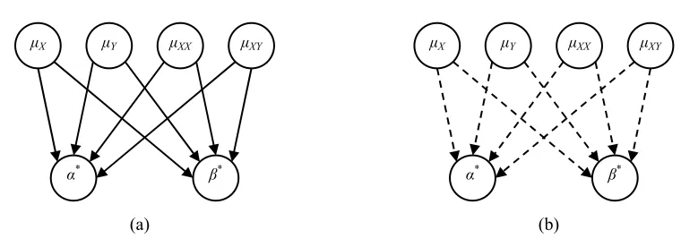
X Y XX XY X Y XX XY

!* "* !* "*

(a) (b)

Figure 1: PCM Directed Acyclic Graphs

3.6.2 SETTABLESYSTEMCAUSALGRAPHS

Given the applicability of the PCM to the unclamped learning example, this system has an associated PCM directed acyclic graph (DAG). The particular representation of this graph depends on whether or not the background variables are observable or not. Figure 1(a) depicts the case of observableγ and Figure 1(b) that of unobservableγ.The solid arrows in Figure 1(a) indicate that the background variables are observable, whereas the dashed arrows in Figure 1(b) indicate that the background variables are not observable.

In interpreting these graphs, note that the arrows, whether solid or dashed, represent the func-tional relationships present. They do not, however, represent causal relations, as in the PCM these are defined to hold only between endogenous variables, and no arrows link the endogenous variables here. Pearl (2000) often uses the term “influence” to refer to situations involving functional depen-dence, but not causal dependence. In this sense, the arrows in these DAGs represent “influences.”

In contrast, due to the lack of a fixed point, the PCM does not apply to the learning with clamping example. Necessarily, the PCM cannot supply a causal graph.

In settable systems, partitions play a key role in constructing causal graphs that represent direct causality relations. To see how, consider our clamped learning example. Here, µY(i.e.,

X

0,2(1)) does not directly cause ˜β∗(

X

2(0)), whereas µX,µX X,µXY,andα(

X

0,1(1),

X

0,3(1),

X

0,4(1),and

X

1(1)) are direct causes of ˜β∗ (

X

2(0)). We can succinctly and unambiguously state these causal relations in terms of settable variables by saying that

X

0,2 does not directly cause

X

2, whereas

X

0,1,

X

0,3,

X

0,4, and

X

1are direct causes of

X

2.

For each block Πb of a partition Π={Πb},we construct a settable system causal graph by

letting nodes correspond to settable variables. If one settable variable directly causes another, we draw an arrow from the node representing the cause to that representing the responding settable variable. Note that in contrast to the DAGs for the PCM, we represent all direct causal links as solid arrows, letting dashed nodes represent unobservable settable variables. The motivation for this is that unobservability is a property of the settable variable (the node), not the links between nodes.

(a)

0,4 0,3

0,2 0,1

1 2

(b)

0,4 0,3

0,2 0,1

1 2

Figure 2: Block-specific Settable System Causal Graphs for the Elementary Partition

0,4 0,3

0,2 0,1

1 2

Figure 3: Settable System Superimposed Causal Graph for the Elementary Partition

For convenience, we may superimpose settable system causal graphs. Superimposing Fig-ures 2(a) and 2(b) gives Figure 3. This is a cyclic graph. Nevertheless, this cyclicality does not represent true simultaneity; it is instead an artifact of the superimposition.

The settable system causal graph for the global partitionΠg={{1,2}}representing unclamped learning is depicted in Figure 4. Observe that this reproduces the connectivity of Figure 1. Note that in Figure 4, the nodes represent settable variables and the arrows represent direct causes. In Figure 1, the nodes represent background or endogenous variables and the arrows represent non-causal “influences.”

We emphasize that the causal graphs associated with settable systems are not necessary to the analysis. Rather, they are sometimes helpful in succinctly representing and studying causal rela-tions.

0,4 0,3

0,2 0,1

1 2

3.7 Further Examples Motivating Settable System Features

We now introduce two further features of settable systems, countable dimension and attributes, using examples involving machine learning algorithms and networks with hidden units. This provides further interesting contrasts between settable systems and the PCM.

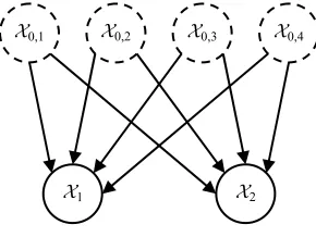
3.7.1 A MACHINELEARNINGALGORITHM ANDCOUNTABLEDIMENSIONALITY

So far, we have restricted attention to the optimal network weights for linear least-squares machine learning. Now consider the machine learning algorithm itself. For this, let

ˆµx,0=ˆµy,0=ˆµxx,0=ˆµxy,0=αˆ0=βˆ0=0, and perform the recursion

ˆµx,n = ˆµx,n−1+n−1(xn−ˆµx,n−1) ˆµy,n = ˆµy,n−1+n−1(yn−ˆµy,n−1)

ˆµxx,n = ˆµxx,n−1+n−1(x2n−ˆµxx,n−1)

ˆµxy,n = ˆµxy,n−1+n−1(xnyn−ˆµxy,n−1) (9) ˆ

βn = 1{ˆµxx,n−ˆµ2x,n>0}[ˆµxx,n−ˆµ

2

x,n]−1(ˆµxy,n−ˆµx,nˆµy,n)

ˆ

αn = ˆµy,n−βˆnˆµx,n, n=1,2, ....

Variables determined outside the system are the observed data sequences x := (x1,x2, ...)and y := (y1,y2, ...).Variables determined within the system are ˆµx:= (ˆµx,0,ˆµx,1, ...),ˆµy:= (ˆµy,0,ˆµy,1, ...),ˆµxx:=

(ˆµxx,0,ˆµxx,1, ...),ˆµxy:= (ˆµxy,0,ˆµxy,1, ...),αˆ = (αˆ0,αˆ1, ...),and ˆβ:= (βˆ0,βˆ1, ...).Under mild conditions, ˆ

αnconverges toα∗and ˆβnconverges toβ∗.

We now ask whether this system falls into the PCM. The answer is no, because the PCM requires the dimensions of the background and endogenous variables to be finite. Here these dimensions are countably infinite. The PCM does not apply. (As a referee notes, however, a countably infinite version of the PCM has recently been discussed by Eichler and Didelez, 2007).

In contrast, settable systems encompass this learning system by permitting the settable variables to be of countably infinite dimension. The definitions of direct causality and the notion of partition-ing operate identically in either the finite or the countably infinite case. Settable systems generally accommodate any recursive learning algorithm involving data sequences of arbitrary length.

3.7.2 LEARNING WITH AHIDDENUNITNETWORK ANDATTRIBUTES

To motivate the next feature of settable systems, we return to considering the effect on an optimal network weight of interventions to distributional parameters,γ,and another network weight. Now, however, we modify the prediction function to be that defined by

f(X ;α,β) =α φ(βX).

input-to-hidden weightβ, and a single hidden-to-output weightα. This elementary structure suffices to make our key points and keeps our notation simple.

Now the expected squared prediction error is

L(α,β,γ;φ):=Eγ([Y−α φ(βX)]2).

Here,γreverts to representing the general parameter indexing F_γ.The choiceγ:= (µX,µY,µX X,µXY)

considered above is no longer appropriate, due to the nonlinearity in network output induced by φ.Further, note the presence of the hidden unit activation functionφin the argument list of L.We make this explicit, asφcertainly helps determine prediction performance, and it has a key role to play in our subsequent discussion.

Now consider the clamped optimization problems corresponding to the elementary partitionΠe. This yields solutions

e

A∗₍β_,γ_;φ_{) : =arg min}

α∈AL(α,β,γ;φ),

e

B∗₍α_,γ_;φ_{) : =arg min}

β∈BL(α,β,γ;φ).

We ensure the existence of compact-valued correspondencesAe∗₍β_,γ_;φ_)andBe∗₍α_,γ_;φ_{)by (among} other things) takingA _andB _{to be compact subsets of}R_{. Elements ˜}α∗ _ofAe∗₍β_,γ_;φ_{) and ˜}β∗ _of e

B∗₍α_,γ_;φ_{)satisfy the necessary first order conditions}

E_γ([φ(βX)]2_)α˜∗_−E

γ(φ(βX)Y) = 0, E_γ(Dφ(β˜∗X)Y)−αE_γ[Dφ(β˜∗X)φ(β˜∗X)] = 0,

where Dφdenotes the first derivative of theφfunction. We caution that although these relations nec-essarily hold for elements ofAe∗₍β_,γ_;φ_)andBe∗₍α_,γ_;φ_{),not all(}α_,β_{)values jointly satisfying these} implicit equations are members of Ae∗₍β_,γ_;φ_{) and}Be∗₍α_,γ_;φ_{).Some solutions to these equations} may be local minima, inflection points, or (local) maxima.

The PCM does not apply here, due (among other things) to the absence of a unique fixed point. Nevertheless, settable systems do apply, using a principled selection of elements fromAe∗₍β_,γ_;φ₎ andBe∗₍α_,γ_;φ_{),respectively. We write these selections}

˜ α∗_=˜r

1(β,γ;φ), β˜∗=˜r2(α,γ;φ).

The feature distinguishing this example from our earlier examples is the appearance in the re-sponse functions of the hidden unit activation functionφ. The key feature ofφis that it takes one and only one value: φis the standard normal density. It is therefore not a variable. Consequently, it cannot be a setting, and it is distinct from any of the other objects we have previously examined. We define an attribute to be any object specified a priori that helps determine responses but is not variable. We associate attributes with the system units. Any attribute of the system itself is a system attribute; we formally associate system attributes to each system unit. Here,φis a system attribute. Because a unit’s associated attributes are constant, they are not subject to counterfactual variation. Nevertheless, attributes may differ across units.

of the system. The identity attribute is required by settable systems, as the identity labels are those explicitly used in the partitioning operation. The identity attribute is also a feature of the PCM, as background and endogenous variables are distinct types of objects, and elements of each distinct type have identifying subscripts.

When attributes beyond identity are present, they need not be distinct across units. For example, the quantity n appearing in several of the response functions in the learning algorithm of Equation (9) is an attribute shared by those units.

We emphasize that attributes are relative to the particular structural system, not somehow ab-solute. Some objects may be taken as attributes solely for convenience. For example, one might consider several different possible activation functions and attempt to learn the best one for a given problem. In such systems, the hidden unit activation is no longer an attribute but is an endogenous variable. In other cases, it may be more convenient to treat the activation function as hard-wired, in which case the activation function is an attribute. Indeed, any hard-wired aspect of the system is properly an attribute. Convenience may even dictate treating as attributes objects that are in prin-ciple variable, but whose degree of variation is small relative to that of other system variables of interest.

Other system aspects are more inherently attributes. Because of their fundamental role and their invariance, such attributes are easily taken for granted and thus overlooked. Our least-squares learning example is a case in point. Specifically, the loss function itself is properly viewed as an attribute.

A useful way to appreciate this is to consider the loss functions

Lp(α,β,γ):= Z

|y−f(x;α,β)|pdFγ(x,y), p>0.

In our examples so far, we always take p=2,so L=L2.Different choices are possible, yielding different loss functions. A leading example is the choice p=1.Whereas p=2 yields forecasts that approximate the conditional mean of Y given X, p=1 yields forecasts that approximate the conditional median of Y given X.

Because p is a constant specified a priori and because p helps determine the optimal responses, p is an attribute. When the forecaster’s goal is explicitly to provide a forecast based on the conditional mean, it makes little sense to consider values of p other than 2,because no other value of p is guaranteed to generally deliver an approximation to the conditional expectation. Put somewhat differently, it may not make much sense to attempt to endogenize p and choose an “optimal” value of p from some set of admissible values because the result of choosing different values for p is to modify the very goal of the learning exercise. Nor can one escape from attributes by endogenizing p; as long as there is some optimality criterion at work, this criterion is properly an attribute of the system.

Another important example of inherent attributes is provided by the sets S_{i that specify the} admissible values taken by the settings

X

i(1) and responses

X

i(0). These are properly specified

a priori; they take one and only one value for each unit i; and they play a fundamental role in determining system responses.

3.7.3 ATTRIBUTES IN THE PCM

In contrast, a somewhat ambiguous situation prevails in the PCM. Viewing attributes as a subset of those objects having no causal status, Pearl (2000, p. 98) states that attributes can be treated as elements of u, the background variables.3 This overlooks the key property we wish to assign to attributes: for a given unit, they are fixed, not variable. Such objects thus cannot belong to u if one takes the word “variable” at face value. In our view, assigning attributes to u misses the opportunity to make an important distinction between invariant aspects of the system units on the one hand and counterfactual variation admissible for the system unit values on the other. Among other things, assigning attributes to u interferes with assigning natural causal roles to structurally exogenous variables.

Further, just as for endogenous and exogenous variables, the PCM does not provide guidance about how to select attributes. In contrast, settable systems clearly identify attributes as invariant features of the system units that embody fundamental aspects of the decision problem represented by the settable system.

Below, we will further distinguish attributes from variables when we discuss stochastic settable systems.

3.8 A Comparative Review of PCM and Settable System Features

At this point, it is helpful to take stock of the features of settable systems that we have so far introduced and contrast these with corresponding features of the PCM.

(1) Settable systems explicitly represent the dual roles of the variables of structural systems us-ing settable variables. These dual roles are present but implicit in the PCM. Settable variables can be responses, or they can be set to given values (settings). The explicit representation of these dual roles in settable systems makes possible implicitly defined structural relations that may not be repre-sentable in the PCM. Further, these implicit structural relations may involve correspondences rather than functions. Principled selections from these correspondences yield unique response functions in settable systems.

(2) In settable systems, all variables of the system, structurally exogenous or endogenous, have causal status, in that they can be potential causes or direct causes. Further, no assumptions are made as to the observability of system variables: structurally exogenous variables may be either observable or unobservable; the same is true for structurally endogenous variables. In particular, this permits settable systems to admit unobserved causes and results in causal relations that are not relative to an observer. In contrast, the PCM admits causal status only for endogenous variables. For the PCM, structurally exogenous unobserved causes are ruled out. Although the PCM does permit treating background variables as endogenous variables in alternative systems, it is silent as to how to distinguish between exogenous and endogenous variables. On the other hand, the governing principles in settable systems provide a formal and explicit means for distinguishing between endogenous and exogenous variables.

(3) Settable systems admit straightforward definitions of interventions and direct effects. These notions, while present, are less direct in the formal PCM.

(4) In settable systems, partitioning permits specification of different mutually consistent ver-sions of a given structural system in which different groups of variables are jointly free to respond to the other variables of the system. In particular, system variables can respond either singly or jointly

to the other variables of the system, as illustrated by our examples of learning with or without clamp-ing. Similar exercises are possible in the PCM using submodels and the do operator, but the PCM requirement of a unique fixed point limits its applicability. Specifically, we saw that learning with clamping falls outside the PCM. Halpern’s (2000) GPCM does apply to such systems, but causal discourse is problematic, due to the absence of the potential response function. In settable systems, fixed points are not required, and causal notions obtain without requiring the potential response function. This permits settable systems to provide causal meaning in our examples of learning with or without clamping.

(5) Settable systems can have a countable infinity of units, whereas the PCM requires a finite number of units.

(6) In settable systems, attributes are a priori constants associated with the units that help deter-mine responses. In the PCM, attributes are not necessarily linked to the system units. Further, they are treated not as constants, but as background variables, resulting in potential ambiguity. The PCM is silent as to how to distinguish between attributes and variables.

Some features of settable systems, such as relaxing the assumption of unique fixed points (point 4) and accommodating an infinity of agents (point 5), are entirely unavailable in the PCM. The remaining settable systems features above rigorously formalize and extend or refine related PCM features and thus permit more explicit causal inference.

4. Stochastic Settable Systems: Heuristics

In the PCM, randomness does not formally appear until definition 7.1.6 (probabilistic causal model). Nevertheless, Pearl’s (2000) definitions 7.1.1 through 7.1.5 (causal model, submodel, effect of ac-tion, potential response, and counterfactual) explicitly refer to “realizations” pa or x of endogenous variables PA or X . These references make sense only if PA and X are interpreted as random vectors. Although u is not explicitly called a realization, the language of definition 7.1.1 further suggests that u is viewed as a realization of random background variables, U . This becomes explicit in definition 7.1.6, where PCM background variables U become governed by a probability measure P. Random-ness of endogenous variables is then induced by their dependence on U . In this sense, definitions 7.1.1 through 7.1.5 do not have fully defined content until definition 7.1.6 resolves the meaning of U,V,PA,and X.Nevertheless, definitions 7.1.1 through 7.1.5 are perfectly meaningful, simply viewing the referenced variables as real numbers.

The settable systems discussed so far are entirely non-stochastic: the settings and responses defined in Section 3 are real numbers, not random variables. Nevertheless, we can connect causal and stochastic structures in settable systems by viewing settings and responses as realizations of random variables, in much the same spirit as the PCM. In this section we discuss some specifics of this connection.

4.1 Introducing Randomness into Settable Systems

settings. Thus, in the hidden unit clamped learning example, we have random responses

˜

A∗=˜r1(B,C;φ), B˜∗=˜r2(A,C;φ).

Second, the underlying probability measure for settable systems can depend on the attribute vector, call it a, of the system. Whereas in the PCM attributes are “lumped together” with other background variables, and may therefore be random, this is not permitted in settable systems. In settable systems, attributes are specified a priori and take one and only one value, a. Because of its a priori status, this value is non-random.

It follows that the probability measure governing the settable system can be indexed by a. This is not an empty possibility; it has clear practical value. One context in which this practical value arises is when attention focuses only on the units of some subsystem of a larger system. For example, consider the least squares machine learning algorithm of the equations in (9), and focus attention on the subsystem

ˆ

B = 1_{Mˆxx−Mˆ2x>0}[

ˆ

Mxx−Mˆx2]−1(Mˆxy−MˆxMˆy),

ˆ

A = Mˆy−B ˆˆMx.

Note that we have modified the notation to reflect the fact that the settings ˆMx,Mˆy,Mˆxx,and ˆMxy

are now random variables. These generate realizations ˆµx,n,ˆµy,n,ˆµxx,n,and ˆµxy,n under a probability

measure Pn,which is that induced by the probability measure governing the random fundamental

settings{(X1,Y1), ...,(Xn,Yn)}.Note the explicit dependence of the probability measure Pnon the

attribute n.The fact that this probability measure can depend on attributes underscores their nature as a priori constants in settable systems.

4.2 Some Formal Properties of Stochastic Settable Systems

Given attributes a, we let(Ω,

F

,Pa)denote the complete probability space on which the settings and

responses are defined. Here,Ωis a set (the “universe”) whose elementsωindex possible outcomes (“possibilities”);

F

is aσ−field of measurable subsets ofΩwhose elements represent events; and Pa is a probability measure (indexed by a) on the measurable space(Ω,

F

)that assigns a number

Pa(F)to each event F∈

F

. See, for example, White (2001, Chap. 3) for an introductory discussion

of measurable spaces and probability spaces.

We decomposeωasω:= (ωr,ωs), withωr∈Ωr,ωs∈Ωs,so thatΩ=Ωr×Ωs. As we discuss

next, this enables distinct components ofωto underlie responses (ωr) and settings (ωs). This

facili-tates straightforward and rigorous definitions of counterfactuals and interventions. These notions in turn support a definition of direct effect.

To motivate the foundations for defining counterfactuals, again consider the hidden unit clamped learning example. Formally, the random settings(A,B,C) are measurable functions A :Ωs→R,

B :Ωs→R,and C :Ωs→Rm,m∈N.Lettingωsbelong toΩs,we take the setting values to be the

realizations

Observe that the settings depend only on theωs component ofω.We make this explicit in A(ωs),

B(ωs),and C(ωs),but leave this implicit in writing

X

0(ω,1),

X

1(ω,1),and

X

2(ω,1)for notational

convenience.

The responses are determined similarly:

˜

A∗(ω) = ˜r1(B(ωs),C(ωs),ωr;φ) =˜r1(

X

2(ω,1),

X

0(ω,1),ωr;φ) =:

X

1(ω,0),

˜

B∗(ω) = ˜r2(A(ωs),C(ωs),ωr;φ) =˜r2(

X

1(ω,1),

X

0(ω,1),ωr;φ) =:

X

2(ω,0).

Note that we now make explicit the possibility that the response functions may depend directly on ωr.This dependence was absent in all our previous examples but is often useful in applications, as

this dependence permits responses to embody an aspect of “pure” randomness. From now on, we will includeωras an explicit argument of the response functions.

In the deterministic systems previously considered, we viewed the fundamental setting

X

0(1) as a primitive object and adopted the convention that

X

0(0):=

X

0(1).Once settings and responses depend onω,it becomes necessary to modify our conventions regarding the fundamental settable variables

X

0,as

X

0 is no longer determined outside the system. The role of the system primitive is now played by ω, the primary setting. We represent this as the settable variable defined by

X

∗(ω,0):=

X

∗(ω,1):=ω. We now view

X

0(ω,0) as a response to ωs and we take

X

0(·,1):=

X

0(·,0).

In the current stochastic framework, the feature that distinguishes

X

0from other settable vari-ables is that the response

X

0(ω,0)depends only onωs,whereas responses of other settable variables

can depend directly on other settings and onωr. Given the availability of

X

∗,there is no guarantee or

requirement that such a settable variable

X

0 exists. Nevertheless, such fundamental stochastic set-table variables

X

0are often an important and useful feature in applications, as our machine learning examples demonstrate.

The definition of direct causality in stochastic settable systems is closely parallel to that in the non-stochastic case. Specifically, consider the partition Π={Πb},and suppose i belongs to the

partition elementΠb.Let

X

(b)(ω,1)denote setting values for the settable variables whose indexes do not belong toΠb,together with the settings

X

0(ω,1).Then the response

X

i(ω,0)is given by

X

i(ω,0):=ri(

X

(b)(ω,1),ωr; a) =ri(z(b),ωr; a),

where riis the associated response function, a is the attribute vector, and for convenience we write

z(b):=

X

(b)(ωs,1).Then we say that

X

jdoes not directly cause

X

iif ri(z(b),ωr; a)defines a function

constant in the element zj of(z(b),ωr)for all values of the other elements of(z(b),ωr).Otherwise,

we say that

X

jdirectly causes

X

i.Thus,

X

∗can directly cause

X

i; for this, take zj=ωr.If

X

0(ω,0) does not define a constant function ofωs,we also say that

X

∗directly causes

X

0.As always, direct causality is relative to the specified partition.

4.3 Counterfactuals, Interventions, and Direct Effects

We now have the foundation necessary to specify “counterfactuals.” We begin by defining what is meant by “factual.” Suppose for now that all setting and response values apart fromωr are

ob-servable. Specifically, suppose we have realizations of setting values (β,γ) and response value ˜

α∗_{=˜r1(β,γ,ω}

r;φ),and thatωis such thatβ=B(ωs),γ=C(ωs),and ˜α∗=A˜∗(ω),where

˜