Complete Identification Methods for the Causal Hierarchy
Ilya Shpitser [email protected]
Judea Pearl [email protected]
Cognitive Systems Laboratory Department of Computer Science University of California, Los Angeles Los Angeles, CA 90095, USA
Editor: Peter Spirtes
Abstract
We consider a hierarchy of queries about causal relationships in graphical models, where each level in the hierarchy requires more detailed information than the one below. The hierarchy consists of three levels: associative relationships, derived from a joint distribution over the observable vari-ables; cause-effect relationships, derived from distributions resulting from external interventions; and counterfactuals, derived from distributions that span multiple “parallel worlds” and resulting from simultaneous, possibly conflicting observations and interventions. We completely character-ize cases where a given causal query can be computed from information lower in the hierarchy, and provide algorithms that accomplish this computation. Specifically, we show when effects of in-terventions can be computed from observational studies, and when probabilities of counterfactuals can be computed from experimental studies. We also provide a graphical characterization of those queries which cannot be computed (by any method) from queries at a lower layer of the hierarchy. Keywords: causality, graphical causal models, identification
1. Introduction
The human mind sees the world in terms of causes and effects. Understanding and mastering our en-vironment hinges on answering questions about cause-effect relationships. In this paper we consider three distinct classes of causal questions forming a hierarchy.
The first class of questions involves associative relationships in domains with uncertainty, for example, “I took an aspirin after dinner, will I wake up with a headache?” The tools needed to formalize and answer such questions are the subject of probability theory and statistics, for they require computing or estimating some aspects of a joint probability distribution. In our aspirin example, this requires estimating the conditional probability P(headache|aspirin)in a population that resembles the subject in question, that is, sharing age, sex, eating habits and any other traits that can be measured. Associational relationships, as is well known, are insufficient for establishing causation. We nevertheless place associative questions at the base of our causal hierarchy, because the probabilistic tools developed in studying such questions are instrumental for computing more informative causal queries, and serve therefore as an easily available starting point from which such computations can begin.
differ, of course from the associational counterpart
P(headache|aspirin), because all mechanisms which normally determine aspirin taking behavior, for example, taste of aspirin, family advice, time pressure, etc. are irrelevant in evaluating the effect of a new decision.
To estimate effects, scientists normally perform randomized experiments where a sample of units drawn from the population of interest is subjected to the specified manipulation directly. In our aspirin example, this might involve treating a group of subjects with aspirin and comparing their response to untreated subjects, both groups being selected at random from a population resembling the decision maker in question. In many cases, however, such a direct approach is not possible due to expense or ethical considerations. Instead, investigators have to rely on observational studies to infer effects. A fundamental question in causal analysis is to determine when effects can be inferred from statistical information, encoded as a joint probability distribution, obtained under normal, intervention-free behavior. A key point here is that in order to make causal inferences from statistics, additional causal assumptions are needed. This is because without any assumptions it is possible to construct multiple “causal stories” which can disagree wildly on what effect a given intervention can have, but agree precisely on all observables. For instance, smoking may be highly correlated with lung cancer either because it causes lung cancer, or because people who are genetically predisposed to smoke may also have a gene responsible for a higher cancer incidence rate. In the latter case there will be no effect of smoking on cancer. Distinguishing between such causal stories requires additional, non-statistical language. In this paper, the language that we use for this purpose is the language of graphs, and our causal assumptions will be encoded by a special directed graph called a causal diagram.
The use of directed graphs to represent causality is a natural idea that arose multiple times in-dependently: in genetics (Wright, 1921), econometrics (Haavelmo, 1943), and artificial intelligence (Pearl, 1988; Spirtes et al., 1993; Pearl, 2000). A causal diagram encodes variables of interest as nodes, and possible direct causal influences between two variables as arrows. Associated with each node in a causal diagram is a stable causal mechanism which determines its value in terms of the values of its parents. Unlike Bayesian networks (Pearl, 1988), the relationships between variables are assumed to be deterministic and uncertainty arises due to the presence of unobserved variables which have influence on our domain.
The first question we consider is under what conditions the effect of a given intervention can be computed from just the joint distribution over observable variables, which is obtainable by statis-tical means, and the causal diagram, which is either provided by a human expert, or inferred from experimental studies. This identification problem has received consideration attention in the statis-tics, epidemiology, and causal inference communities (Pearl, 1993a; Spirtes et al., 1993; Pearl and Robins, 1995; Pearl, 1995; Kuroki and Miyakawa, 1999; Pearl, 2000). In the subsequent sections, we solve the identification problem for causal effects by providing a graphical characterization for all non-identifiable effects, and an algorithm for computing all identifiable effects. Note that this identification problem actually involves two “worlds:” the original world where no interventions took place furnishes us with a probability distribution from which to make inferences about the sec-ond, post-intervention world. The crucial feature of causal effect queries which distinguishes them from more complex questions in our hierarchy is that they are restricted to the post-intervention world alone.
interventions or observations. An example of such a question would be “I took an aspirin, and my headache is gone; would I have had a headache had I not taken that aspirin?” Unlike questions involving interventions, counterfactuals contain conflicting information: in one world aspirin was taken, in another it was not. It is unclear therefore how to set up an effective experimental procedure for evaluating counterfactuals, let alone how to compute counterfactuals from observations alone. If everything about our causal domain is known, in other words if we have knowledge of both the causal mechanisms and the distributions over unobservable variables, it is possible to compute counterfactual questions directly (Balke and Pearl, 1994b). However, knowledge of precise causal mechanisms is not generally available, and the very nature of unobserved variables means their stochastic behavior cannot be estimated directly. We therefore consider the more practical question of how to compute counterfactual questions from both experimental studies and the structure of the causal diagram.
It may seem strange, in light of what we said earlier about the difficulty of conducting experi-mental studies, that we take such studies as given. It is nevertheless important that we understand when it is that “what-if” questions involving multiple worlds can be inferred from quantities com-putable in one world. Our hierarchical approach to identification allows us to cleanly separate difficulties that arise due to multiplicity of worlds from those involved in the identification of causal effects. We provide a complete solution to this version of the identification problem by giving algo-rithms which compute identifiable counterfactuals from experimental studies, and provide graphical conditions for the class of non-identifiable counterfactuals, where our algorithms fail. Our results can, of course, be combined to give conditions where counterfactuals can be computed from obser-vational studies.
The paper is organized as follows. Section 2 introduces the notation and mathematical machin-ery needed for causal analysis. Section 3 considers the problem of identifying causal effects from observational studies. Section 4 considers identification of counterfactual queries, while Section 5 summarizes the conclusions. Most of the proofs are deferred to the appendix. This paper consoli-dates and expands previous results (Shpitser and Pearl, 2006a,b, 2007). Some of the results found in this paper were also derived independently elsewhere (Huang and Valtorta, 2006b,a).
2. Notation and Definitions
The primary object of causal inquiry is a probabilistic causal model. We will denote variables by uppercase letters, and their values by lowercase letters. Similarly, sets of variables will be denoted by bold uppercase, and sets of values by bold lowercase.
Definition 1 A probabilistic causal model (PCM) is a tuple M=hU,V,F,P(u)i, where
• U is a set of background or exogenous variables, which cannot be observed or experimented on, but which affect the rest of the model.
• V is a set{V1, ...,Vn}of observable or endogenous variables. These variables are functionally
dependent on some subset of U∪V.
• F is a set of functions{f1, ...,fn}such that each fiis a mapping from a subset of U∪V\ {Vi}
to Vi, and such thatSF is a function from U to V.
The set of functions F in this definition corresponds to the causal mechanisms, while U rep-resents the background context that influences the observable domain of discourse V, yet remains outside it. Our ignorance of the background context is represented by a distribution P(u). This distribution, together with the mechanisms in F, induces a distribution P(v)over the observable do-main. The causal diagram, our vehicle for expressing causal assumptions, is defined by the causal model as follows. Each observable variable Vi∈V corresponds to a vertex in the graph. Any two variables Vi∈U∪V, Vj∈V such that Viappears in the description of fjare connected by a directed arrow from Vito Vj. Furthermore, we make two additional assumptions in this paper. The first is that
P(u) =∏ui∈u P(ui), and each Ui∈U is used in at most two functions in F.1 The second is that all induced graphs must be acyclic. Models in which these two assumptions hold are called recursive semi-Markovian. A graph defined as above from a causal model M is said to be a causal diagram
induced by M. Graphs induced by semi-Markovian models are themselves called semi-Markovian.
Fig. 1 and Fig. 2 show some examples of causal diagrams of recursive semi-Markovian models.
The functions in F are assumed to be modular in a sense that changes to one function do not affect any other. This assumption allows us to model how a PCM would react to changes imposed from the outside. The simplest change that is possible for causal mechanisms of a variable set X would be one that removes the mechanisms entirely and sets X to a specific value x. This change, denoted by do(x)(Pearl, 2000), is called an intervention. An intervention do(x)applied to a model
M results in a submodel Mx. The effects of interventions will be formulated in several ways. For any
given u, the effect of do(x)on a set of variables Y will be represented by counterfactual variables
Yx(u), where Y ∈Y. As U varies, the counterfactuals Yx(u) will vary as well, and their
interven-tional distribution, denoted by P(y|do(x))or Px(y)will be used to define the effect of x on Y. We will denote the event “variable Y attains value y in Mx” by the shorthand yx.
Interventional distributions are a mathematical formalization of an intuitive notion of effect of action. We now define joint probabilities on counterfactuals, in multiple worlds, which will serve as the formalization of counterfactual queries. Consider a conjunction of eventsγ=y1x1∧...∧ykxk.
If all the subscripts xi are the same and equal to x,γis simply a set of assignments of values to variables in Mx, and P(γ) =Px(y1, ...,yk). However, if the actions do(xi) are not the same, and potentially contradictory, a single submodel is no longer sufficient. Instead, γis really invoking multiple causal worlds, each represented by a submodel Mxi. We assume each submodel shares
the same set of exogenous variables U, corresponding to the shared causal context or background history of the hypothetical worlds. Because the submodels are linked by common context, they can really be considered as one large causal model, with its own induced graph, and joint distribution over observable variables. P(γ)can then be defined as a marginal distribution in this causal model. Formally, P(γ) =∑{u|u|=γ}P(u), where u|=γis taken to mean that each variable assignment in
γholds true in the corresponding submodel of M when the exogenous variables U assume values u. In this way, P(u) induces a distribution on all possible counterfactual variables in M. In this paper, we will represent counterfactual utterances by joint distributions such as P(γ)or conditional distributions such as P(γ|δ), whereγandδare conjunctions of counterfactual events. Pearl (2000) discusses counterfactuals, and their probabilistic representation used in this paper in greater depth.
1. Our results are generalizable to other P(u)distributions which may not have such a simple form, but which can be
A fundamental question in causal inference is whether a given causal question, either inter-ventional or counterfactual in nature, can be uniquely specified by the assumptions embodied in the causal diagram, and easily available information, usually statistical, associated with the causal model. To get a handle on this question, we introduce an important notion of identifiability (Pearl, 2000).
Definition 2 (identifiability) Consider a class of models M with a description T , and objectsφand θcomputable from each model. We say thatφisθ-identified in T ifφis uniquely computable from θin any M∈M. In this case all models in M which agree onθwill also agree onφ.
If φis θ-identifiable in T , we write T,θ`id φ. Otherwise, we write T,θ6`id φ. The above definition leads immediately to the following corollary which we will use to prove non-identifiability results.
Corollary 3 Let T be a description of a class of models M. Assume there exist M1,M2∈M that share objectsθ, whileφin M1is different fromφin M2. Then T,θ6`idφ.
In our context, the objects φ,θ are probability distributions derived from the PCM, where θ represents available information, whileφrepresents the quantity of interest. The description T is a specification of the properties shared all causal models under consideration, or, in other words, the set of assumptions we wish to impose on those models. Since we chose causal graphs as a language for specifying assumptions, T corresponds to a given graph.
Graphs earn their ubiquity as a specification language because they reflect in many ways the way people store experiential knowledge, especially cause-effect relationships. The ease with which people embrace graphical metaphors for causal and probabilistic notions—ancestry, neighborhood, flow, and so on—are proof of this affinity, and help ensure that the assumptions specified are mean-ingful and reliable. A consequence of this is that probabilistic dependencies among variables can be verified by checking if the flow of influence is blocked along paths linking the variables. By a path we mean a sequence of distinct nodes where each node is connected to the next in the sequence by an edge. The precise way in which the flow of dependence can be blocked is defined by the notion of d-separation (Pearl, 1986; Verma, 1986; Pearl, 1988). Here we generalize d-separation somewhat to account for the presence of bidirected arcs in causal diagrams.
Definition 4 (d-separation) A path p in G is said to be d-separated by a set Z if and only if either
1 p contains one of the following three patterns of edges: I→M→J, I↔M→J, or I←M→ J, such that M∈Z, or
2 p contains one of the following three patterns of edges: I→M←J, I↔M←J, I↔M↔J, such that De(M)G∩Z=/0.
(e)
Z X
Y
Z1
Z2 X
Y
(g) (f)
Y Z X
Y
(h)
Z
W X X
Y
(a) (b)
X
Y Z
X
Y Z
(c) (d)
Y Z X
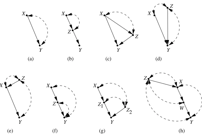
Figure 1: Causal graphs where P(y|do(x))is not identifiable
to its conditional distribution given the values of its parents in the graph. In other words, P(v,u) = ∏iP(xi|pa(xi)G).
Whenever the above factor decomposition holds for a distribution P(v,u) and a graph G, we say G is an I-map of P(v,u). The following theorem links d-separation of vertex sets in an I-map G with the independence of corresponding variable sets in P.
Theorem 5 If sets X and Y are d-separated by Z in G, then X is independent of Y given Z in every
P for which G is an I-map. Furthermore, the causal diagram induced by any semi-Markovian PCM M is an I-map of the distribution P(v,u)induced by M.
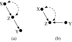
Note that it’s easy to rephrase the above theorem in terms of ordinary directed acyclic graphs, since each semi-Markovian graph is really an abbreviation where each bidirected arc stands for two directed arcs emanating from a hidden common cause. We will abbreviate this statement of d-separation, and corresponding independence by(X⊥⊥Y|Z)G, following the notation of Dawid (1979). For example in the graph shown in Fig. 6 (a), X 6⊥⊥Y and X ⊥⊥Y|Z, while in Fig. 6 (b), X⊥⊥Y and X6⊥⊥Y|Z.
Finally we consider the axioms and inference rules we will need. Since PCMs contain proba-bility distributions, the inference rules we would use to compute queries in PCMs would certainly include the standard axioms of probability. They also include a set of axioms which govern the be-havior of counterfactuals, such as Effectiveness, Composition, etc. (Galles and Pearl, 1998; Halpern, 2000; Pearl, 2000). However, in this paper, we will concentrate on a set of three identities applicable to interventional distributions known as do-calculus (Pearl, 1993b, 2000):
• Rule 1: Px(y|z,w) =Px(y|w)if(Y⊥⊥Z|X,W)Gx
• Rule 3: Px,z(y|w) =Px(y|w)if(Y⊥⊥Z|X,W)Gx,z(w) where Z(W)= Z\An(W)G
X, and Gx,y stands for a directed graph obtained from G by removing all incoming arrows to X and all outgoing arrows from Y. The rules of do-calculus provide a way of linking ordinary statistical distributions with distributions resulting from various manipulations.
In the remainder of this section we will introduce relevant graphs and graph-theoretic terminol-ogy which we will use in the rest of the paper. First, having defined causal diagrams induced by natural causal models, we consider the graphs induced by models derived from interventional and counterfactual queries. We note that in a given submodel Mx, the mechanisms determining X no longer make use of the parents of X to determine their values, but instead set them independently to constant values x. This means that the induced graph of Mx derived from a model M inducing graph
G can be obtained from G by removing all arrows incoming to X, in other words Mx induces Gx.
A counterfactual γ=y1x1∧...∧ykxk, as we already discussed invokes multiple hypothetical causal
worlds, each represented by a submodel, where all worlds share the same background context U. A naive way to graphically represent these worlds would be to consider all the graphs G
Xi and have them share the U nodes. It turns out this representation suffers from certain problems. In Section 4 we discuss this issue in more detail and suggest a more appropriate graphical representation of counterfactual situations.
We denote Pa(.)G,Ch(.)G,An(.)G,De(.)Gas the sets of parents, children, ancestors, and descen-dants of a given set in G. We denote GX to be the subgraph of G containing all vertices in X, and edges between these vertices, while the set of vertices in a given graph G is given by ver(G). As a shorthand, we denote Gver(G)\ver(G0)as G\G0or G\X, if X=ver(G0), and G0is a subgraph of G. We will call the set{X ∈G|De(X)G=/0}the root set of G. A path connecting X and Y which begins with an arrow pointing to X is called a back-door path from X , while a path beginning with an arrow pointing away from X is called a front-door path from X .
The goal of this paper is a complete characterization of causal graphs which permit the answer-ing of causal queries of a given type. This characterization requires the introduction of certain key graph structures.
Definition 6 (tree) A graph G such that each vertex has at most one child, and only one vertex
(called the root) has no children is called a tree.
Note that this definition reverses the usual direction of arrows in trees as they are generally understood in graph theory. If we ignore bidirected arcs, graphs in Fig. 1 (a), (b), (d), (e), (f), (g), and (h) are trees.
Definition 7 (forest) A graph G such that each vertex has at most one child is called a forest. Note that the above two definitions reverse the arrow directionality usual for these structures.
Definition 8 (confounded path) A path where all directed arrowheads point at observable nodes,
and never away from observable nodes is called a confounded path.
The graph in Fig. 1 (g) contains a confounded path from Z1to Z2.
Definition 9 (c-component) A graph G where any pair of observable nodes is connected by a
X
Y
(a)
Y Z X
(d)
X
Y
X
Y Z
Z1
Z2
Y
(g)
Z3 X
X
Y Z
(e)
X
Y Z
(b) (c)
Z1
Z2
(f)
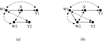
Figure 2: Causal graphs admitting identifiable effect P(y|do(x))
Graphs in Fig. 1 (a), (d), (e), (f), and (h) are components. Some graphs contain multiple c-components, for example the graph in Fig. 1 (b) has two maximal c-components:{Y}, and{X,Z}. We will denote the set of maximal c-components of a given graph G by C(G). The importance of c-components stems from the fact that that the observational distribution P(v)can be expressed as a product of factors Pv\s(s), where each s is a set of nodes forming a c-component. This impor-tant property is known as c-component factorization, and we will this property extensively in the remainder of the manuscript to decompose identification problems into smaller subproblems.
In the following sections, we will show how the graph structures we defined in this section are key for characterizing cases when Px(y)and P(γ)can be identified from available information.
3. Identification of Causal Effects
Like probabilistic dependence, the notion of causal effect of X on Y has an interpretation in terms of flow. Intuitively, X has an effect on Y if changing X causes Y to change. Since intervening on X cuts off X from the normal causal influences of its parents in the graph, we can interpret the causal effect of X on Y as the flow of dependence which leaves X via outgoing arrows only.
Recall that our ultimate goal is to express distributions of the form P(y|do(x))in terms of the joint distribution P(v). The interpretation of effect as downward dependence immediately suggests a set of graphs where this is possible. Specifically, whenever all d-connected paths from X to Y are front-door from X, the causal effect P(y|do(x))is equal to P(y|x). In graphs shown in Fig. 2 (a) and (b) causal effect P(y|do(x))has this property.
In general, we don’t expect acting on X to produce the same effect as observing X due to the presence of back-door paths between X and Y. However, d-separation gives us a way to block undesirable paths by conditioning. If we can find a set Z that blocks all back-door paths from X to Y, we obtain the following: P(y|do(x)) =∑z P(y|z,do(x))P(z|do(x)). The term P(y|z,do(x))
adjusting for Z introduced a new effect we must compute, corresponding to the term P(z|do(x)). If it so happens that no variable in Z is a descendant of X, we can reduce this term to P(z)using the intuitive argument that acting on effects should not influence causes, or a more formal appeal to rule 3 of do-calculus. Computing effects in this way is always possible if we can find a set Z blocking all back-door paths which contains no descendants of X. This is known as the back-door criterion (Pearl, 1993a, 2000). Figs. 2 (c) and (d) show some graphs where the node z satisfies the back-door criterion with respect to P(y|do(x)), which means P(y|do(x))is identifiable.
The back-door criterion can fail—a common way involves a confounder that is unobserved, which prevents adjusting for it. Surprisingly, it is sometimes possible to identify the effect of X on Y even in the presence of such a confounder. To do so, we want to find a set Z located downstream of X but upstream of Y, such that the downward flow of the effect of X on Y can be decomposed into the flow from X to Z, and the flow from Z to Y. Clearly, in order for this to happen Z must d-separate all front-door paths from X to Y. However, in order to make sure that the component effects P(z|do(x))and P(y|do(z))are themselves identifiable, and combine appropriately to form
P(y|do(x)), we need two additional assumptions: there are no back-door paths from X to Z, and all back-door paths from Z to Y are blocked by X. It turns out that these three conditions imply that P(y|do(x)) =∑z P(y|do(z))P(z|do(x)), and the latter two conditions further imply that the first term is identifiable by the back-door criterion and equal to∑z P(y|z,x)P(x), while the second term is equal to P(z|x). Whenever these three conditions hold, the effect of X on Y is identifiable. This is known as the front-door criterion (Pearl, 1995, 2000). The front-door criterion holds in the graph shown in Fig. 2 (e).
Unfortunately, in some graphs neither the front-door, nor the back-door criterion holds. The simplest such graph, known as the bow arc graph due to its shape, is shown in Fig. 1 (a). The back-door criterion fails since the confounder node is unobservable, while the front-door criterion fails since no intermediate variables between X and Y exist in the graph. While the failure of these two criteria does not imply non-identification, in fact the effect P(y|do(x))is identifiable in Fig. 2 (f), (g) despite this failure, a simple argument shows that P(y|do(x))is not identifiable in the bow arc graph.
Theorem 10 P(v),G6`idP(y|do(x))in G shown in Fig. 1 (a).
Since we are interested in completely characterizing graphs where a given causal effect P(y|do(x))
is identifiable, it would be desirable to list difficult graphs like the bow arc graph which prevent iden-tification of causal effects, in the hope of eventually making such a list complete and finding a way to identify effects in all graphs not on the list. We start constructing this list by considering graphs which generalize the bow arc graph since they can contain more than two nodes, but which also inherit its difficult structure. We call such graphs C-trees.
Definition 11 (C-tree) A graph G which is both a C-component and a tree is called a C-tree. We call a C-tree with a root node Y Y -rooted. The graphs in Fig. 1 (a), (d), (e), (f), and (h) are
Y -rooted C-trees. It turns out that in any Y -rooted C-tree, the effect of any subset of nodes, other
than Y , on the root Y is not identifiable.
Theorem 12 Let G be a Y -rooted C-tree. Let X be any subset of observable nodes in G which does
C-trees play a prominent role in the identification of direct effects. Intuitively, the direct effect of X on Y exists if there is an arrow from X to Y in the graph, and corresponds to the flow of influence along this arrow. However, simply considering changes in Y after fixing X is insufficient for isolating direct effect, since X can influence Y along other, longer front-door paths than the direct arrow. In order to disregard such influences, we also fix all other parents of Y (which as noted earlier removes all arrows incoming to these parents and thus to Y ). The expression corresponding to the direct effect of X on Y is then P(y|do(pa(y))). The following theorem links C-trees and direct effects.
Theorem 13 P(v),G6`id P(y|do(pa(y)))if and only if there exists a subgraph of G which is a Y
-rooted C-tree.
This theorem might suggest that C-trees might play an equally strong role in identifying arbitrary effects on a single variable, not just direct effects. Unfortunately, this turns out not to be the case, due to the following lemma.
Lemma 14 (downward extension lemma) Let V be the set of observable nodes in G, and P(v)the observable distribution of models inducing G. Assume P(v),G6`id P(y|do(x)). Let G0 contain all
the nodes and edges of G, and an additional node Z which is a child of all nodes in Y. Then if P(v,z) is the observable distribution of models inducing G0, then P(v,z),G06`idP(z|do(x)).
Proof Let|Z|=∏Y
i∈Y|Yi|=n. By construction, P(z|do(x)) =∑y P(z|y)P(y|do(x)). Due to the
way we set the arity of Z, P(Z|Y)is an n by n matrix which acts as a linear map which transforms
P(y|do(x))into P(z|do(x)). Since we can arrange this linear map to be one to one, any proof of non-identifiability of P(y|do(x))immediately extends to the proof of non-identifiability of P(z|do(x)).
What this lemma shows is that identification of effects on a singleton is not any simpler than the general problem of identification of effect on a set. To find difficult graphs which prevent identification of effects on sets, we consider a multi-root generalization of C-trees.
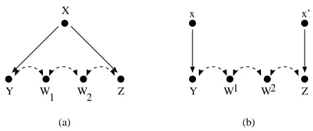
Definition 15 (c-forest) A graph G which is both a C-component and a forest is called a C-forest. If a given C-forest has a set of root nodes R, we call it R-rooted. Graphs in Fig. 3 (a), (b) are
{Y 1,Y 2}-rooted C-forests. A naive way to generalize Theorem 12 would be to state that if G is an R-rooted C-forest, then the effect of any set X that does not intersect R is not identifiable. However, as we later show, this is not true. Specifically, we later prove that P(y1,y2|do(x))in the graph in Fig. 3 (a) is identifiable. To formulate the correct generalization of Theorem 12, we must understand what made C-trees difficult for the purposes of identifying effects on the root Y . It turned out that for particular function choices, the effects of ancestors of Y on Y precisely cancelled themselves out so even though Y itself was dependent on its parents, it was observationally indistinguishable from a constant function. To get the same canceling of effects with C-forests, we must define a more complex graphical structure.
Definition 16 (hedge) Let X,Y be sets of variables in G. Let F,F0be R-rooted C-forests in G such that F0 is a subgraph of F, X only occur in F, and R∈An(Y)Gx. Then F and F0 form a hedge for
(a) (b)
W1 X
Y1
W2 Y2
W1 X
Y1
W2 Y2
Figure 3: (a) A graph hedge-less for P(y|do(x)). (b) A graph containing a hedge for P(y|do(x)).
The graph in Fig. 3 (b) contains a hedge for P(y1,y2|do(x)). The mental picture for a hedge is as follows. We start with a C-forest F0. Then, F0grows new branches, while retaining the same root set, and becomes F. Finally, we “trim the hedge,” by performing the action do(x)which has the effect of removing some incoming arrows in F\F0(the subgraph of F consisting of vertices not a part of F0). Note that any Y -rooted C-tree and its root node Y form a hedge. The right generalization of Theorem 12 can be stated on hedges.
Theorem 17 Let F,F0 be subgraphs of G which form a hedge for P(y|do(x)). Then P(v),G6`id
P(y|do(x)).
Proof outline As before, assume binary variables. We let the causal mechanisms of one of the mod-els consists entirely of bit parity functions. The second model also computes bit parity for every mechanism, except those nodes in F0which have parents in F ignore the values of those parents. It turns out that these two models are observationally indistinguishable. Furthermore, any intervention in F\F0will break the bit parity circuits of the models. This break will be felt at the root set R of the first model, but not of the second, by construction.
Unlike the bow arc graph, and C-trees, hedges prevent identification of effects on multiple variables at once. Certainly a complete list of all possible difficult graphs must contain structures like hedges. But are there other kinds of structures that present problems? It turns out that the answer is “no,” any time an effect is not identifiable in a causal model (if we make no restrictions on the type of function that can appear), there is a hedge structure involved. To prove that this is so, we need an algorithm which can identify any causal effect lacking a hedge. This algorithm, which we call ID, and which can be viewed as a simplified version of the identification algorithm due to Tian (2002), appears in Fig. 4.
We will explain why each line of ID makes sense, and conclude by showing the operation of the algorithm on an example. The formal proof of soundness of ID can be found in the appendix. The first line merely asserts that if no action has been taken, the effect on Y is just the marginal of the observational distribution P(v) on Y. The second line states that if we are interested in the effect on Y, it is sufficient to restrict our attention on the parts of the model ancestral to Y. One intuitive argument for this is that descendants of Y can be viewed as ’noisy versions’ of Y and so any information they may impart which may be helpful for identification is already present in Y. On the other hand, variables which are neither ancestors nor descendants of Y lie outside the relevant causal chain entirely, and have no useful information to contribute.
function ID(y, x, P, G)
INPUT: x,y value assignments, P a probability distribution, G a causal diagram.
OUTPUT: Expression for Px(y)in terms of P or FAIL(F,F’).
1 if x=/0return∑v\y P(v). 2 if V\An(Y)G6= /0
return ID(y,x∩An(Y)G,∑v\An(Y)GP,GAn(Y)). 3 let W= (V\X)\An(Y)Gx.
if W6=/0, return ID(y,x∪w,P,G). 4 if C(G\X) ={S1, ...,Sk}
return∑v\(y∪x)∏iID(si,v\si,P,G). if C(G\X) ={S}
5 if C(G) ={G}, throw FAIL(G,G∩S).
6 if S∈C(G)return∑s\y∏{i|Vi∈S}P(vi|v
(i−1)
π ). 7 if(∃S0)S⊂S0∈C(G)return ID(y,x∩S0,
∏{i|Vi∈S0}P(Vi|V
(i−1)
π ∩S0,vπ(i−1)\S0),GS0).
Figure 4: A complete identification algorithm. FAIL propagates through recursive calls like an exception, and returns the hedge which witnesses non-identifiability. Vπ(i−1)is the set of nodes preceding Viin some topological orderingπin G.
the causal graph we consider by removing certain arcs from the graph, without affecting the overall answer. Line 4 is the key line of the algorithm, it decomposes the problem into a set of smaller problems using the key property of c-component factorization of causal models. If the entire graph is a single C-component already, further problem decomposition is impossible, and we must provide base cases. ID has three base cases. Line 5 fails because it finds two C-components, the graph G itself, and a subgraph S that does not contain any X nodes. But that is exactly one of the properties of C-forests that make up a hedge. In fact, it turns out that it is always possible to recover a hedge from these two c-components. Line 6 asserts that if there are no bidirected arcs from X to the other nodes in the current subproblem under consideration, then we can replace acting on X by conditioning, and thus solve the subproblem. Line 7 is the most complex case where X is partitioned into two sets, W which contain bidirected arcs into other nodes in the subproblem, and Z which do not. In this situation, identifying P(y|do(x))from P(v) is equivalent to identifying P(y|do(w))from
P(V|do(z)), since P(y|do(x)) =P(y|do(w),do(z)). But the term P(V|do(z))is identifiable using the previous base case, so we can consider the subproblem of identifying P(y|do(w)).
We give an example of the operation of the algorithm by identifying Px(y1,y2)from P(v)in the graph shown in in Fig. 3 (a). Since G=GAn({Y1,Y2}),C(G\ {X}) ={G}, and W={W1}, we invoke
W1 X Y1
(a) (b)
W1 Y1
Figure 5: Subgraphs of G used for identifying Px(y1,y2).
4. Thus the original problem reduces to identifying∑w2Px,w1,w2,y2(y1)Pw,x,y1(w2,y2). Solving for the
second expression, we trigger line 2, noting that we can ignore nodes which are not ancestors of W2 and Y2, which means Pw,x,y1(w2,y2) =P(w2,y2). Solving for the first expression, we first trigger line
2 also, obtaining Px,w1,w2,y2(y1) =Px,w(y1). The corresponding G is shown in Fig. 5 (a). Next, we
trigger line 7, reducing the problem to computing Pw(y1)from P(Y1|X,W1)P(W1). The correspond-ing G is shown in Fig. 5 (b). Finally, we trigger line 2, obtaincorrespond-ing Pw(y1) =∑w1P(y1|x,w1)P(w1).
Putting everything together, we obtain: Px(y1,y2) =∑w2P(y1,w2)∑w1P(y1|x,w1)P(w1).
As mentioned earlier, whenever the algorithm fails at line 5, it is possible to recover a hedge from the C-components S and G considered for the subproblem where the failure occurs. In fact, it can be shown that this hedge implies the non-identifiability of the original query with which the algorithm was invoked, which implies the following result.
Theorem 18 ID is complete.
The completeness of ID implies that hedges can be used to characterize all cases where effects of the form P(y|do(x))cannot be identified from the observational distribution P(v).
Theorem 19 (hedge criterion) P(v),G6`id P(y|do(x))if and only if G contains a hedge for some
P(y0|do(x0)), where y0⊆y, x0⊆x.
We close this section by considering identification of conditional effects of the form P(y|do(x),z)
which are defined to be equal to P(y,z|do(x))/P(z|do(x)). Such expressions are a formalization of an intuitive notion of “effect of action in the presence of non-contradictory evidence,” for instance the effect of smoking on lung cancer incidence rates in a particular age group (as opposed to the effect of smoking on cancer in the general population). We say that evidence z is non-contradictory since it is conceivable to consider questions where the evidence z stands in logical contradiction to the proposed hypothetical action do(x): for instance what is the effect of smoking on cancer among the non-smokers. Such counterfactual questions will be considered in the next section. Condition-ing can both help and hinder identifiability. P(y|do(x))is not identifiable in the graph shown in Fig. 6 (a), while it is identifiable in the graph shown in Fig. 6 (b). Conditioning reverses the situation. In Fig. 6 (a), conditioning on Z renders Y independent of any changes to X , making Px(y|z)equal to
P(y|z). On the other hand, in Fig. 6 (b), conditioning on Z makes X and Y dependent, resulting in
Px(y|z)becoming non-identifiable.
(a) (b) X
X Z
Z Y
Y
Figure 6: (a) Causal graph with an identifiable conditional effect P(y|do(x),z). (b) Causal graph with a non-identifiable conditional effect P(y|do(x),z).
function IDC(y, x, z, P, G)
INPUT: x,y,z value assignments, P a probability distribution, G a causal diagram (an I-map of P).
OUTPUT: Expression for Px(y|z)in terms of P or FAIL(F,F’). 1 if(∃Z∈Z)(Y⊥⊥Z|X,Z\ {Z})Gx,z,
return IDC(y,x∪ {z},z\ {z},P,G). 2 else let P0=ID(y∪z,x,P,G).
return P0/∑y P0.
Figure 7: A complete identification algorithm for conditional effects.
Theorem 20 For any G and any conditional effect Px(y|w)there exists a unique maximal set Z= {Z∈W|Px(y|w) =Px,z(y|w\ {z})}such that rule 2 applies to Z in G for Px(y|w). In other words,
Px(y|w) =Px,z(y|w\z).
Of course Theorem 20 does not guarantee that the entire set z can be handled in this way. In many cases, even after rule 2 is applied, some set of evidence will remain in the expression. Fortunately, the following result implies that identification of unconditional causal effects is all we need.
Theorem 21 Let Z⊆W be the maximal set such that Px(y|w) =Px,z(y|w\z). Then Px(y|w) is identifiable in G if and only if Px,z(y,w\z)is identifiable in G.
The previous two theorems suggest a simple addition to ID, which we call IDC, shown in Fig. 7, which handles identification of conditional causal effects.
Theorem 22 IDC is sound and complete. Proof This follows from Theorems 20 and 21.
(a) (b) A
H H H*
A=false A*=true
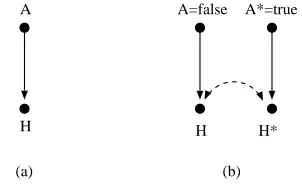
Figure 8: (a) A causal graph for the aspirin/headache domain (b) A corresponding twin network graph for the query P(Ha∗∗=true|A= f alse).
Theorem 23 The rules of do-calculus are complete for identifying effects of the form P(y|do(x),z), where x,y,z are arbitrary sets.
Proof The proofs of soundness of ID and IDC in the appendix use do-calculus. This implies every line of the algorithms we presented can be rephrased as a sequence of do-calculus manipulations. But ID and IDC are also complete, which implies the conclusion.
4. Identification of Counterfactuals
While effects of actions have an intuitive interpretation as downward flow, the interpretation of counterfactuals, or what-if questions is more complex. An informal counterfactual statement in natural language such as “would I have a headache had I taken an aspirin” talks about multiple worlds: the actual world, and other, hypothetical worlds which differ in some small respect from the actual world (e.g., the aspirin was taken), while in most other respects are the same. In this paper, we represent the actual world by a causal model in its natural state, devoid of any interventions, while the alternative worlds are represented by submodels Mx where the action do(x)implements the hypothetical change from the actual state of affairs considered. People make sense of informal statements involving multiple, possibly conflicting worlds because they expect not only the causal rules to be invariant across these worlds (e.g., aspirin helps headaches in all worlds), but the worlds themselves to be similar enough where evidence in one world has ramifications in another. For instance, if we find ourselves with a headache, we expect the usual causes of our headache to also operate in the hypothetical world, interacting there with the preventative influence of aspirin. In our representation of counterfactuals, we model this interaction between worlds by assuming that the world histories or background contexts, represented by the unobserved U variables are shared across all hypothetical worlds.
We illustrate the representation method for counterfactuals we introduced in Section 2 by mod-eling our example question “would I have a headache had I taken an aspirin?” The actual world referenced by this query is represented by a causal model containing two variables, headache and aspirin, with aspirin being a parent of headache, see Fig. 8 (a). In this world, we observe that aspirin has value false. The hypothetical world is represented by a submodel where the action
single causal model with the graph shown in Fig. 8 (b). Our query is represented by the distribution
P(Ha∗∗=true|A= f alse), where H is headache, and A is aspirin. Note that the nodes A∗=true and A=f alse in Fig. 8 (b) do not share a bidirected arc. This is because an intervention do(a∗=true)
removes all incoming arrows to A∗, which removes the bidirected arc between A∗and A.
The graphs representing two hypothetical worlds invoked by a counterfactual query like the one shown in Fig. 8 (b) are called twin network graphs, and were first proposed as a way to represent counterfactuals by Balke and Pearl (1994b) and Balke and Pearl (1994a). In addition, Balke and Pearl (1994b) proposed a method for evaluating expressions like P(Ha∗∗=true|A= f alse) when all
parameters of a causal model are known. This method can be explained as follows. If we forget the causal and counterfactual meaning behind the twin network graph, and simply view it as a Bayesian network, the query P(Ha∗∗=true|A= f alse) can be evaluated using any of the standard inference
algorithms available, provided we have access to all conditional probability tables generated by F and U of a causal model which gave rise to the twin network graph. In practice, however, complete knowledge of the model is too much to ask for; the functional relationships as well as the distribution
P(u) are not known exactly, though some of their aspects can be inferred from the observable distribution P(v).
Instead, the typical state of knowledge of a causal domain is the statistical behavior of the ob-servable variables in the domain, summarized by the distribution P(v), together with knowledge of causal directionality, obtained either from expert judgment (e.g., we know that visiting the doctor does not make us sick, though disease and doctor visits are highly correlated), or direct experi-mentation (e.g., it’s easy to imagine an experiment which establishes that wet grass does not cause sprinklers to turn on). We already used these two sources of knowledge in the previous section as a basis for computing causal effects. Nevertheless, there are reasons to consider computing counter-factual quantities from experimental, rather than observational studies. In general, a countercounter-factual can posit worlds with features contradictory to what has actually been observed. For instance, ques-tions resembling the headache/aspirin question we used as an example are actually frequently asked in epidemiology in the more general form where we are interested in estimating the effect of a treat-ment x on the outcome variable Y for the patients that were not treated (x0). In our notation, this is just our familiar expression P(Yx|X =x0). The problem with questions such as these is that no experimental setup exists in which someone is both given and not given treatment. Therefore, it makes sense to ask under what circumstances we can evaluate such questions even if we are given as input every experiment that is possible to perform in principle on a given causal model. In our framework the set of all experiments is denoted as P∗, and is formally defined as{Px|x is any set of values of X⊆V}. The question that we ask in this section, then, is whether it is possible to identify a query P(γ|δ), whereγ,δare conjunctions of counterfactual events (withδpossibly empty), from the graph G and the set of all experiments P∗. We can pose the problem in this way without loss of generality since we already developed complete methods for identifying members of P∗from G and
P(v). This means that if for some reason using P∗as input is not realistic we can combine the meth-ods which we will develop in this section with those in the previous section to obtain identification results for P(γ|δ)from G and P(v).
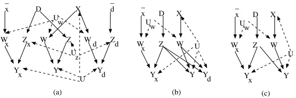
Y Z W Y Z W X x x x (b) D x D Y Z W X d d d d U w U z d U U U Y Z W X U (a)
D x d
Y Z W X x (c) U x D x _ _ _ (d) Y z W X x,z U x,z x _ _
Figure 9: Nodes fixed by actions denoted with an overline, signifying that all incoming arrows are cut. (a) Original causal diagram (b) Parallel worlds graph for P(yx|x0,zd,d)(the two nodes denoted by U are the same). (c) Counterfactual graph for P(yx|x0,zd,d). (d) Counterfac-tual graph for P(yx,z|x0).
query of interest would involve three or more worlds. For instance, we might be interested in how likely the patient would be to have a symptom Y given a certain dose x of drug X , assuming we know that the patient has taken dose x0of drug X , dose d of drug D, and we know how an interme-diate symptom Z responds to treatment d. This would correspond to the query P(yx|x0,zd,d), which mentions three worlds, the original model M, and the submodels Md,Mx. This problem is easy to tackle—we simply add more than two submodel graphs, and have them all share the same U nodes. This simple generalization of the twin network model was considered by Avin et al. (2005), and was called there the parallel worlds graph. Fig. 9 shows the original causal graph and the parallel worlds graph forγ=yx∧x0∧zd∧d.
The other problematic feature of the twin network graph, which is inherited by the parallel worlds graph, is that multiple nodes can sometimes correspond to the same random variable. For example, in Fig. 9 (b), the variables Z and Zxare represented by distinct nodes, although it’s easy to show that since Z is not a descendant of X , Z=Zx. These equality constraints among nodes can make the d-separation criterion misleading if not used carefully. For instance, Yx ⊥⊥Dx|Z even though using d-separation in the parallel worlds graph suggests the opposite. This sort of problem is fairly common in causal models which are not faithful (Spirtes et al., 1993) or stable (Pearl, 2000), in other words in models where d-separation statements in a causal diagram imply independence in a distribution, but not vice versa. However, lack of faithfulness usually arises due to “numeric coincidences” in the observable distribution. In this case, the lack of faithfulness is “structural,” in a sense that it is possible to refine parallel worlds graphs in such a way that the node duplication disappears, and the attendant independencies not captured by d-separation are captured by d-separation in refined graphs.
gen-erally much smaller and less cluttered than parallel worlds graphs, and so are easier to understand. Compare, for instance, the graphs in Fig. 9 (b) and Fig. 9 (c). To rid ourselves of duplicates, we need a formal way of determining when variables from different submodels are in fact the same. The following lemma does this.
Lemma 24 Let M be a model inducing G containing variablesα,βwith the following properties: • αandβhave the same domain of values.
• There is a bijection f from Pa(α)to Pa(β)such that a parentγand f(γ)have the same domain of values.
• The functional mechanisms ofαandβare the same (except whenever the function forαuses the parentγ, the corresponding function forβuses f(γ)).
Assume an observable variable set Z was observed to attain values z in Mx, the submodel obtained from M by forcing another observable variable set X to attain values x. Assume further that for eachγ∈Pa(α), either f(γ) =γ, orγand f(γ) attain the same values (whether by observation or intervention). Thenαandβare the same random variable in Mx with observations z.
Proof This follows from the fact that variables in a causal model are functionally determined from their parents.
If two distinct nodes in a causal diagram represent the same random variable, the diagram con-tains redundant information, and the nodes must be merged. If two nodes, say corresponding to
Yx,Yz, are established to be the same in G, they are merged into a single node which inherits all
the children of the original two. These two nodes either share their parents (by induction) or their parents attain the same values. If a given parent is shared, it becomes the parent of the new node. Otherwise, we pick one of the parents arbitrarily to become the parent of the new node. This oper-ation is summarized by the following lemma.
Lemma 25 Let Mx be a submodel derived from M with set Z observed to attain values z, such that
Lemma 24 holds forα,β. Let M0 be a causal model obtained from M by mergingα,βinto a new nodeω, which inherits all parents and the functional mechanism ofα. All children of α,βin M0 become children ofω. Then Mx,Mx agree on any distribution consistent with z being observed.0
Proof This is a direct consequence of Lemma 24.
The new nodeωwe obtain from Lemma 25 can be thought of as a new counterfactual variable. As mentioned in section 2, such variables take the form Yx where Y is the variable in the original causal model, and x is a subscript specifying the action which distinguishes the counterfactual. Since we only merge two variables derived from the same original, specifying Y is simple. But what about the subscript? Intuitively, the subscript ofω contains those fixed variables which are ancestors ofω in the graph G0 of M0. Formally the subscript is w, where W=An(ω)G0∩sub(γ),
function make-cg(G,γ)
INPUT: G a causal diagram,γa conjunction of counterfactual events
OUTPUT: A counterfactual graph Gγ, and either a set of events γ0 s.t. P(γ0) = P(γ) or INCONSISTENT
• Construct a submodel graph Gxi for each action do(xi)mentioned inγ. Construct the parallel
worlds graph G0by having all such submodel graphs share their corresponding U nodes.
• Letπbe a topological ordering of nodes in G0, letγ0:=γ.
• Apply Lemmas 24 and 25, in orderπ, to each observable node pairα,βderived from the same variable in G. For eachα,βthat are the same, do:
– Let G0be modified as specified in Lemma 25. – Modifyγ0by renaming all occurrences ofβtoα. – If val(α)6=val(β), return G0,INCONSISTENT.
• return(G0An(γ0),γ0), where An(γ0)is the set of nodes in G0ancestral to nodes corresponding to
variables mentioned inγ0.
Figure 10: An algorithm for constructing counterfactual graphs
Note that sinceα,βare the same, their value assignments must be the same (say equal to y). The new counterfactualωinherits this assignment.
We summarize the inductive applications of Lemma 24, and 25 by the make-cg algorithm, which takesγand G as arguments, and constructs a version of the parallel worlds graph without duplicate nodes. We call the resulting structure the counter f actual graph ofγ, and denote it by Gγ. The algorithm is shown in Fig. 10.
There are three additional subtleties in make-cg. The first is that if variables Yx,Yz were judged
to be the same by Lemma 24, butγassigns them different values, this implies that the original set of counterfactual eventsγis inconsistent, and so P(γ) =0. The second is that if we are interested in identifiability of P(γ), we can restrict ourselves to the ancestors ofγin G0. We can justify this using the same intuitive argument we used in Section 3 to justify Line 2 in ID. The formal proof for line 2 we provide in the appendix applies with little change to make-cg. Finally, because the algorithm can make an arbitrary choice picking a parent ofωeach time Lemma 25 is applied, both the counterfactual graph G0, and the corresponding modified counterfactualγ0are not unique. This does not present a problem, however, as any such graph is acceptable for our purposes.
Y Z W Y Z W x x x (a) Y Z W d d d Uw Uz U x d _ _ D Y Z W Y W x x (b) x _ X D X U w U Y d Y Z W Y W x x (c) x _ D X U w U
Figure 11: Intermediate graphs obtained by make-cg in constructing the counterfactual graph for
P(yx|x0,zd,d)from Fig. 9 (b).
has a single child, that variable is omitted from the graph. For instance, in Fig. 11 (a), the variable
Ud, and its corresponding arrow to D omitted.
Next, we apply Lemma 24 for the node pair Wd,W . In this case, the functional mechanisms are once again the same, while the parents of Wd,W are X and Uw. We can also apply Lemma 24 twice to conclude that Z,Zxand Zdare in fact the same node, and so can be merged. The functional mechanisms of these three nodes are the same, and they share the parent Uz. As far as the parents of this triplet, the Uzparent is shared by all three, while Z,Zxshare the parent D, and Zdhas a separate parent d, fixed by intervention. However, in our counterfactual query, which is P(yx|x0,zd,d), the variable D happens to be observed to attain the value d, the same as the intervention value for the parent of Zd. This implies that for the purposes of the Z,Zx,Zdtriplet, their D-derived parents share the same value, which allows us to conclude they are the same random variable. The intuition here is that while intervention and observation are not the same operation, they have the same effect if the relevant U variables happen to react in the same way to both the given intervention, and the given observation (this is the essence of the Axiom of Composition discussed by Pearl (2000).) In our case, U variables react the same way because the parallel worlds share all unobserved variables.
There is one additional subtlety in performing the merge of the triplet Z,Zx,Zd. If we examine our query P(yx|x0,zd,d), we notice that Zd, or more precisely its value, appears in it. When we merge nodes, we only use one name out of the original two. It’s possible that some of the old names appear in the query, which means we must replace all references to the old, pre-merge nodes with the new post-merge name we picked. Since we picked the name Z for the newly merged node, we replace the reference to Zdin our query by the reference to Z, so our modified query is P(yx|x0,z,d). Since the variables were established to be the same, this is a safe syntactic transformation.
After Wd,W , and the Z,Zx,Zd triplet are merged, we obtain the graph in Fig. 11 (b). Finally, we apply Lemma 24 one more time to conclude Y and Yd are the same variable, using the same reasoning as before. After performing this final merge, we obtain the graph in Fig. 11 (c). It’s easy to see that Lemma 24 no longer applies to any node pair: W and Wxdiffer in their X -derived parent, and
function ID*(G,γ)
INPUT: G a causal diagram,γa conjunction of counterfactual events OUTPUT: an expression for P(γ)in terms of P∗or FAIL
1 ifγ=/0, return 1
2 if(∃xx0..∈γ), return 0
3 if(∃xx..∈γ), return ID*(G,γ\ {xx..})
4 (G0,γ0) =make-cg(G,γ)
5 ifγ0=INCONSISTENT, return 0 6 if C(G0) ={S1, ...,Sk},
return∑V(G0)\γ0∏iID*(G,si
v(G0)\si)
7 if C(G0) ={S}then,
8 if(∃x,x0)s.t. x6=x0,x∈sub(S),x0∈ev(S), throw FAIL
9 else, let x=S sub(S)
return Px(var(S))
function IDC*(G,γ,δ)
INPUT: G a causal diagram,γ,δconjunctions of counterfactual events OUTPUT: an expression for P(γ|δ) in terms of P∗, FAIL, or UNDEFINED
1 if ID*(G,δ) =0, return UNDEFINED
2 (G0,γ0∧δ0) =make-cg(G,γ∧δ)
3 ifγ0∧δ0=INCONSISTENT, return 0 4 if(∃yx∈δ0)s.t.(Yx⊥⊥γ0)G0
yx, return IDC*(G,γ0
yx,δ0\ {yx})
5 else, let P0=ID*(G,γ0∧δ0). return P0/P0(δ)
Figure 12: Counterfactual identification algorithms.
obtained. In our case, we remove nodes W and Y (and their adjacent edges) from consideration, to finally obtain the graph in Fig. 9 (c), which is a counterfactual graph for our query.
These algorithms make use of the following notation: sub(.)returns the set of subscripts, var(.)
the set of variables, and ev(.)the set of values (either set or observed) appearing in a given coun-terfactual conjunction (or set of councoun-terfactual events), while val(.)is the value assigned to a given counterfactual variable. This notation is used to extract variables and values present in the original causal model from a counterfactual which refers to parallel worlds. As before, C(G0)is the set of maximal C-components of G0, except we don’t count nodes in G0 fixed by interventions as part of any C-component. V(G0)is the set of observable nodes of G0 not fixed by interventions. Follow-ing Pearl (2000), G0yx is the graph obtained from G0 by removing all outgoing arcs from Yx;γ0yx is obtained fromγ0by replacing all descendant variables Wz of Yx inγ0 by Wz,y. A counterfactual sr, where s,r are value assignments to sets of nodes, represents the event “the node set S attains values s under intervention do(r).” For instance, the term siv(g0)\si stands for the event “the node set Si
attains values siunder the intervention do(v(g0)\si),” in other words under the intervention where we fix the values of all observable nodes in G0except those in Si. Finally, we take xx..to mean some
counterfactual variable derived from X where x appears in the subscript (the rest of the subscript can be arbitrary), which also attains value x.
The notation used in these algorithms is somewhat intricate, so we give an intuitive description of each line. We start with ID*. The first line states that ifγis an empty conjunction, then its prob-ability is 1, by convention. The second line states that ifγcontains a counterfactual which violates the Axiom of Effectiveness (Pearl, 2000), thenγis inconsistent, and we return probability 0. The third line states that if a counterfactual contains its own value in the subscript, then it is a tautolog-ical event, and it can be removed fromγwithout affecting its probability. Line 4 invokes make-cg to construct a counterfactual graph G0, and the corresponding relabeled counterfactual γ0. Line 5 returns probability 0 if an inconsistency was found during the construction of the counterfactual graph, for example, if two variables found to be the same inγhad different value assignments. Line 6 is analogous to Line 4 in the ID algorithm, it decomposes the problem into a set of subproblems, one for each C-component in the counterfactual graph. In the ID algorithm, the term corresponding to a given C-component Siof the causal diagram was the effect of all variables not in Sion variables in Si, in other words Pv\si(si), and the outermost summation on line 4 was over values of variables
not in Y,X. Here, the term corresponding to a given C-component Si of the counterfactual graph
G0 is the conjunction of counterfactual variables where each variable contains in its subscript all variables not in the C-component Si, in other words v(G0)\si, and the outermost summation is over observable variables not inγ0, that is over v(G0)\γ0, where we interpretγ0as a set of counterfactuals, rather than a conjunction. Line 7 is the base case, where our counterfactual graph has a single C-component. There are two cases, corresponding to line 8 and line 9. Line 8 says that ifγ0contains a “conflict,” that is an inconsistent value assignment where at least one value is in the subscript, then we fail. Line 9 says if there are no conflicts, then its safe to take the union of all subscripts inγ0, and return the effect of the subscripts inγ0on the variables inγ0.