2014
Hamiltonicity and $\sigma$-hypergraphs
Christina Zarb
University of Malta, [email protected]
Follow this and additional works at:
https://digitalcommons.georgiasouthern.edu/tag
Part of the
Discrete Mathematics and Combinatorics Commons
This article is brought to you for free and open access by the Journals at Digital Commons@Georgia Southern. It has been accepted for inclusion in Theory and Applications of Graphs by an authorized administrator of Digital Commons@Georgia Southern. For more information, please contact [email protected].
Recommended Citation
Zarb, Christina (2014) "Hamiltonicity and $\sigma$-hypergraphs,"Theory and Applications of Graphs: Vol. 1 : Iss. 1 , Article 1. DOI: 10.20429/tag.2014.010101
Cover Page Footnote
I would like to thank the referees whose comments helped me improve the presentation of this paper.
Abstract
We define and study a special type of hypergraph. Aσ-hypergraphH =H(n, r, q|σ), where
σ is a partition of r, is anr-uniform hypergraph having nq vertices partitioned into n classes ofq vertices each. If the classes are denoted byV1, V2,...,Vn, then a subsetK of V(H) of size
r is an edge if the partition of r formed by the non-zero cardinalities | K ∩ Vi |, 1≤ i ≤n, is σ. The non-empty intersections K ∩ Vi are called the parts of K, and s(σ) denotes the number of parts. We consider various types of cycles in hypergraphs such as Berge cycles and sharp cycles in which only consecutive edges have a nonempty intersection. We show that most
σ-hypergraphs contain a Hamiltonian Berge cycle and that, for n ≥s+ 1 and q ≥ r(r−1), a σ-hypergraph H always contains a sharp Hamiltonian cycle. We also extend this result to
k-intersecting cycles.
1
Introduction
LetV ={v1, v2, ..., vn}be a finite set, and letE={E1, E2, ..., Em}be a family of subsets ofV. The
pair H = (X, E) is called a hypergraph with vertex-set V(H) = V, and with edge-setE(H) =E. When all the subsets are of the same size r, we say that H is an r-uniform hypergraph. A σ -hypergraph H =H(n, r, q |σ), where σ is a partition of r, is an r-uniform hypergraph having nq
vertices partitioned intonclasses ofq vertices each. If the classes are denoted byV1,V2,...,Vn, then
a subsetK ofV(H) of sizeris an edge if the partition ofr formed by the non-zero cardinalities|K
∩Vi |, 1≤i≤n, isσ. The non-empty intersectionsK ∩Vi are called theparts ofK, ands=s(σ)
denotes the number of parts. We denote the largest part ofσ by ∆ = ∆(σ) and the smallest part by δ =δ(σ). In order to avoid trivial situations where there are no edges, we shall always assume thatq ≥∆ andn≥s. These hypergraphs were first introduced in [2] and studied further in [3, 4]. We consider Hamiltonian cycles in σ-hypergraphs. In a graphG, a Hamiltonian path is a path which includes every vertex v ∈ V(G). A Hamiltonian cycle is a closed Hamiltonian path. It is well-known that the problem of determining whether a Hamiltonian cycle exists in a graph is
N P-complete. An excellent survey on results related to Hamiltonicity is given in [5].
In hypergraphs, in particular r-uniform hypergraphs, there are several different types of paths and cycles to consider — amongst the first to be defined was the Berge cycle [1]. A sequence
C= (v1, e1, v2, e2, . . . , vp, ep, v1) is a Berge cycle if
• v1, v2, . . . , vp are all distinct vertices
• e1, e2, . . . , ep are all distinct edges
• vk, vk+1∈ek fork= 1, . . . , p wherevp+1 =v1
A Berge cycle is Hamiltonian if p is equal to the number of vertices.
Several other types of cycles and Hamiltonian cycles have been described and studied as in [7, 8, 10]. The presentation [6] gives an excellent survey of cycles and paths in hypergraphs. We give the following definitions of cycles and Hamiltonian cycles which are particularly suited to the structure of σ-hypergraphs.
Consider anr-uniform hypergraph H. LetC = (e1, . . . , ep) be a sequence of edges of H. Then
C is a sharp cycle if |ei ∩ei+1|> 0 for 1≤ i ≤p, where addition is modulo p, and |ei∩ej|= 0
otherwise.
A sharp cycle C is a sharp Hamiltonian cycle ifV(C) =V(H).
A sharp Hamiltonian cycle C = (e1, e2, . . . , ep) is said to be (t, z)-sharp ifp= 0 (mod 2) and,
for some t, z >0, |ei∩ei+1|=twhen i= 1 (mod 2) and|ei∩ei+1|=z when i= 0 (mod 2), for
cycles are analogous tot-overlapping cycles as described in [9]. A 1-sharp cycle is often referred in the literature to as a loose cycle.
Finally, a k-intersecting cycle C = (e1, e2, . . . , ep) is such that
|ei∩ei+1∩. . .∩ei+k−1|>0
for 1 ≤ i ≤ p, where addition is modulo p, while any other collection of k or more edges has an empty intersection. If V(C) =V(H) then C is a k-intersecting Hamiltonian cycle. Thus a sharp Hamiltonian cycle is a 2-intersecting Hamiltonian cycle.
In this paper we consider all the above types of Hamiltonian cycles inσ-hypergraphs. We first consider Berge cycles, and then move on to sharp Hamiltonian cycles, and finally tok-intersecting cycles. We give some conditions for the existence and non-existence of the different types of Hamiltonian cycles inσ-hypergraphs, which then lead us to consider conditions on the parameters of H=H(n, r, q|σ) for which the different types of Hamiltonian cycles always exist.
When constructing sharp Hamiltonian cycles, we will use matchings — the link between match-ings and Hamiltonian cycles in r-uniform hypergraphs has been extensively studied [1]. Given an
r-uniform hypergraph H, a matching is a set of pairwise vertex-disjoint edges M ⊂ E(H). A
perfect matching is a matching which covers all vertices of H and we denote the size of the largest matching in anr-uniform hypergraph H by ν(H).
Matchings inσ-hypergraphs were studied in [4] and, as in that paper we here give more structure to the vertices of the hypergraph H =H(n, r, q|σ) withσ = (a1, a2, . . . , as), and ∆ =a1 ≥a2 ≥ . . .≥as =δ. The classes making up the vertex set are ordered as V1, V2, . . . , Vn and, within each
Vi, the vertices are ordered asv1,i, v2,i, . . . , vq,i. We visualise the vertex set V(H) as a q×n grid
whose first row isv1,1, v1,2, . . . , v1,n. We sometimes refer to the verticesv1,i, v2,i, . . . , vk,ias the top
k vertices of the class Vi, and to vq−k+1,i, vq−k+2,i, . . . , vq,i as the bottom k vertices of Vi. The
vertices vk,i and vk+1,i are said to be consecutive in Vi. The class V1 is called the first class of
vertices, and Vn is the last class; Vi and Vi+1 are said to be consecutive classes. A set of vertices
contained in h consecutive rows and k consecutive classes ofV(H) is said to be anh×k subgrid of V(H). Also, for σ = (a1, a2, . . . , as), if a1 = a2 =. . . = as = ∆, σ is said to be a rectangular
partition. Furthermore, ifσ is rectangular and ∆ =s(σ), thenσ is asquare partition.
It is well known that in a graph, the Hamiltonian cycle yields a perfect or near perfect (leaving one vertex unmatched if nis odd) matching. In [4], it was shown that there exist arbitrarily large
σ-hypergraphs which do not have a perfect matching, and for which the number of unmatched vertices is quite large. We state a result from this paper:
Lemma 1.1. Let H =H(n, r, q|σ), where σ = (a1, . . . , as), n≥s and q ≥r. Suppose gcd(σ) =
d≥2, and q =t (modd) where 1≤t≤d−1. Then in a maximum matching of H, there are at least tn vertices left unmatched. Hence ν(H)≤ n(q−tr ).
In the sequel, we will show that these σ-hypergraphs, however, still have both a Berge and a sharp Hamiltonian cycle whenq and nare large enough.
2
Berge Cycles
Let us first consider this type of cycle, and give necessary and sufficient conditions for the existence of Hamiltonian Berge cycles in σ-hypergraphs.
Theorem 2.1. Let H =H(n, r, q| σ) with σ = (a1, a2, . . . , as), s≥ 2 and ∆ =a1 ≥a2 ≥ . . .≥ as=δ ≥1. If σ is not rectangular and q ≥∆ and n≥s, then H has Hamiltonian Berge cycle. If
Proof. Let us take a partitionσ which is not rectangular — we construct a Berge cycle as follows: for e1, we take the bottom a1 vertices in V1, the bottom a2 vertices in V2 and so on up to the
bottom as vertices inVs. Fore2, we “shift” the edge one column to the right so that the parts are
taken from V2 toVs+1. We carry on in this fashion, and when we take partas−1 fromVn then we
take partas from V1, but “shift” one row up. We carry on in this way, shifting one column to the
right each time, and shifting one row up each time — when we reach the top row then we start using the bottom vertices again. In all, we form nq distinct edges in this way. We can now order the vertices by labelling the bottom vertex in V1 asv1, the bottom vertex in V2 as v2, and so on
up to the bottom vertex inVnasvn— we then move up one row and label the vertices in this row
vn+1 up tov2n, from left to right, and we carry on in this fashion until we have labelled all vertices
in this way.
Then the cycle v1, e1, v2, e2, . . . , vnq, enq, v1 is a Hamiltonian Berge cycle.
If σ is rectangular and q = ∆ and n = s, then there is only one edge and hence no Berge Hamiltonian cycle, otherwise the Berge Hamiltonian cycle can be constructed as above.
Note: The conditions are easily seen to be necessary, that is ifH has a Berge Hamiltonian cycle then necessarily q ≥∆ and n≥sotherwise H has no edges, while whenσ is rectangular, q must be at least ∆ + 1 and n≥s+ 1, otherwise there are not enough edges.
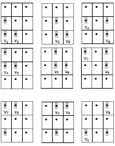
Figure 1 gives an example of a Hamiltonian Berge cycle for H =H(n, r, q|σ) with σ = (2,1),
s= 2 andq =n= 3. The cycle has 9 edges. The shaded vertices form the edge in each case, and the vertices are numbered in cyclic order.
3
Sharp Hamiltonian Cycles
We have given necessary and sufficient conditions for aσ-hypergraph to contain a Berge Hamiltonian cycle. Hence we now turn our attention to sharp Hamiltonian cycles which prove to be more challenging. Although we shall be studying, in a later section, k-intersecting Hamiltonian cycles, we want to treat separately sharp cycles first, which are k-intersecting for k = 2, because they illustrate very clearly the main techniques used in this paper and also because stronger results are possible with sharp cycles, when, in some cases, we prove that the Hamiltonian cycles obtained are eithert-sharp or (t, z)-sharp.
We first present some basic observations about sharp Hamiltonian cycles in r-uniform hyper-graphs.
Lemma 3.1. LetH be ar-uniform hypergraph and letC be a sharp Hamiltonian cycle inH. Then
1. 2|Vr(H)| ≥ |E(C)| ≥ |Vr−(H1)|
2. ν(H)≥ν(C) =
j|E (C)|
2 k
.
3. If 2ν(H) + 1< r−nq1, there is no sharp Hamiltonian cycle in H. Proof.
1. ConsiderC = (e1, e2, . . . , ep). Clearly, each edge of C intersects the next edge, so each edge
contributes at most r−1 vertices to V(C) = V(H), and hence |V(H)| ≤ p(r −1) which imples
p=|E(C)| ≥ |Vr−(H1)|.
Now consider the degrees of the vertices in C. No vertex can have degree greater than 2, so using the well known fact that
r|E(C)|=XdegC(v)≤2|V(H)|
we get the result|E(C)| ≤ 2|Vr(H)|.
2. By the definition of a sharp cycle, the subset ofE(C){e2j+1 : 0≤j≤ j|E
(C)| 2
k
}is a maximal matching inC, as the edges are distinct, and clearly any other edge inC will intersect one of these edges. Hence
ν(H)≥ν(C) =
|E(C)| 2
.
3. If we apply the result in part 1 to σ-hypergraphs, whereV(H) =nq, we get 2nq
r ≥ |E(C)| ≥ nq r−1. Clearly, by the assumption 2ν(H) + 1< r−nq1,
|E(C)| ≥ nq
r−1 >2ν(H) + 1≥2ν(C) + 1. But |E(C)|is an integer, hence
|E(C)| ≥ 2ν(H) + 2≥2ν(C) + 2
= 2
| E(C)|
2
+ 2≥2
|
E(C)| −1 2
+ 2
= |E(C)|+ 1,
3.1 Examples of σ-hypergraphs with no Hamiltonian cycle.
Let us consider examples ofσ-hypergraphs in which there is no sharp Hamiltonian cycle.
For the first example we use Lemma 3.1 — consider H =H(n, r, q|σ) withσ= (∆,∆, . . . ,∆) and s(σ) = ∆≥2, that is σ is a square partition. Letn=q= 2∆−1.
In this case, it is easy to see that ν(H) = 1, while r−nq1 = (2∆∆2−−1)12. Hence, if
(2∆−1)2
∆2−1 >3, that
is for ∆≥3, there is no sharp Hamiltonian cycle in H.
As a second example, consider H = H(n, r, q | σ) with σ = (∆,1, . . . ,1) where s(σ) = ∆ =
r+1
2 ≥ 4 andq =n= r+1
2 . Consider an edge E1 with the first part of size ∆ taken from V1, and
the other parts taken fromV2 toVnrespectively. It is clear that any other edge intersects this edge
— we need at least four edges for a sharp Hamiltonian cycle, but this is impossible since all these edges intersect E1 and hence the cycle is not sharp.
In view of the above examples, our goal is to deal with the following problem which now arises naturally:
Problem 3.1. Let H =H(n, r, q|σ), where s(σ)≥2. Does there exists q(σ) and n(σ) such that for all q≥q(σ) andn≥n(σ),H has a sharp Hamiltonian cycle?
We will supply an affirmative solution to this problem. So we begin with some results which will then allow us to find a solution to this problem.
Lemma 3.2. LetH =H(n, r, q|σ) withσ = (a1, a2, . . . , as), s≥2 and∆ =a1 ≥a2≥. . .≥as=
δ≥1. Let 1≤p < s, and let
t=
i=p X
i=1
ai and z= i=s X
i=p+1
ai =r−t.
If r|q andn≥s+ 1, then H has a (t, z)-sharp Hamiltonian cycle. Moreover if there existsp such that
t=
i=p X
i=1 ai =
i=s X
i=p+1 ai,
then the cycle is t-sharp.
Proof. Let us consider the firstrvertices inV1, . . . , Vnas anr×ngrid of vertices. We will construct
two perfect matchingsM andM∗, whose edges will then be used to form a sharp Hamiltonian cycle
C1 with 2nedges. Observe that we need s=s(σ)≥2, otherwise ifs= 1, that is σ= (r), then for n≥2 H is not connected, while for n= 1, H is the complete r-uniform hypergraph on q vertices, which is trivially Hamiltonian forq ≥r+ 1.
For the first matching M, let each column of r vertices be partitioned into sconsecutive parts of sizesa1, a2, . . . , as (from top to bottom). The partai inVj will be referred to as theith part in
Vj. The edge E1 is formed by taking the top a1 vertices fromV1, the second part of size a2 from V2 and so on, “in diagonal fashion”. This is repeated forE2 by “shifting one class to the right”,
taking the topa1 vertices fromV2, the second part fromV3 etc. In general, the edgeEj, 1≤j≤n,
takes the first part from Vj, the second part from Vj+1 and in general the kth part fromVj+k−1,
for 1≤k≤s, with addition modulon. This gives a perfect matching M withnedges. For the second matching M∗, let 1≤p < s, and let
t=
i=p X
i=1
ai and z= i=s X
i=p+1
Then we take edgeE1∗ such that parts a1 to ap are taken as in edgeE1, while part ap+1 toas are
taken as in edge E2 - this is possible sincen≥s+ 1 and henceE1∗ is different from allEi inM. In
general,Ei∗ has partsa1 toap as in edge Ei, and parts ap+1 toas as in edgeEi+1, where addition
is modulo n. It is clear that these edges form another perfect matching, and that they are distinct from the edges taken inM.
Now a sharp cycleC1 is formed by taking the edges inM ∪M∗ in this order:
E1, E1∗, E2, E2∗, . . . , Ei, Ei∗, Ei+1, Ei∗+1, . . . , En, En∗.
In general,|Ei∩Ei∗|=a1+. . .+ap =tand |Ei∗∩Ei+1|=ap+1+. . .+as=z=r−t, and at the
end, En∗ has parts ap+1 to as to coincide with the same parts in E1 to close the cycle. It is clear
that the cycle is (t, z)-sharp since the only intersections between edges are the ones described. If there existsp such that
t=
i=p X
i=1 ai =
i=s X
i=p+1
ai =z=r−t,
then the cycle ist-sharp.
Now if q ≥r, then for the next r vertices in V1 toVn we can create another sharp cycleC2 in
the same way. To linkC1 toC2, for the last edge ofM∗ inC1, we change the parts ap+1 toas to
coincide with the equivalent parts in the first edge of M inC2, thus linking the two cycles.
Hence ifq=xr, we proceed this way to obtain a sharp Hamiltonian cycleC =C1∪C2∪. . .∪Cx,
where we change the parts ap+1 to as in the last edge of Cx to coincide with the corresponding
parts in the first edge of C1, thus forming a (t, z)-sharp Hamiltonian cycle inH.
Now if there exists psuch that
t=
i=p X
i=1 ai =
i=s X
i=p+1 ai,
it is clear that the cycle ist-sharp.
Lemma 3.3. LetH =H(n, r, q|σ) withσ = (a1, a2, . . . , as), s≥2 and∆ =a1 ≥a2≥. . .≥as=
δ≥1. Let 1≤p < s, and let
t=
i=p X
i=1
ai and z= i=s X
i=p+1
ai =r−t.
If r+ 1|q and n≥s+ 1, then H has an(t−1, z)-sharp Hamiltonian cycle.
Proof. Let us first consider the first r+ 1 vertices in V1, . . . , Vn as an (r+ 1)×n grid of vertices.
As in the previous Lemma, we will construct two matchings M and M∗, whose edges can be used to form a sharp cycleC1 with 2nedges.
The first matching M is constructed in exactly the same way asM was constructed in Lemma 3.2 to cover the topr×ngrid of vertices, havingnedges and leaving out the vertices in the (r+ 1)th row.
For the second matching M∗, again we take 1≤p < s, and let
t=
i=p X
i=1
ai and z= i=s X
i=p+1
The edges are then formed as follows: for edgeE1∗, parta1 is taken as inE1, but replacing the last
vertex in this part with the (r+ 1)th vertex in the same class. Partsa
2 toap are taken as per edge
E1, while parts ap+1 toas are taken as per edge E2. Therefore, in general, Ei∗ has part a1 taken
from Vi to include the top a1−1 vertices, and the last vertex in the class, parts a2 to ap as per
edgeEi , and parts ap+1 toas as in edgeEi+1.
Now the sharp cycle is C1 = (E1, E1∗, E2, E2∗, . . . , En, En∗) so that |Ei∩Ei∗|=t−1, and |Ei∗∩
Ei+1|=z=r−t. The last edgeEn∗ intersects E1 in parts ap+1 toas.
Now ifq ≥r+ 1 and (r+ 1)|q, then for the nextr+ 1 vertices inV1 toVnwe can create another
cycle C2 in the same way. To link C1 to C2, for En∗, we change the parts ap+1 to as to coincide
with the equivalent parts in the first edge ofM inC2, thus linking the two cycles.
Hence if q = x(r+ 1), we proceed this way to obtain a sharp Hamiltonian cycle C = C1 ∪ C2∪. . .∪Cx, where we change the parts ap+1 to as in the last edge of Cx to coincide with the
corresponding parts in the first edge of C1, thus forming a (t−1, z)-sharp Hamiltonian cycle inH.
Again, if there exists psuch that
t−1 =
i=p X
i=1 ai
!
−1 =
i=s X
i=p+1 ai,
then the cycle is (t−1)-sharp.
We shall use the following classical theorem by Frobenius which states:
Theorem 3.4. Let a1, a2 be positive integers withgcd(a1, a2) = 1. Then forn≥(a1−1)(a2−1),
there are nonnegative integers x andy such thatxa1+ya2=n.
Using Lemmas 3.2 and 3.3 combined with Theorem 3.4, we can now present an affirmative solution to Problem 3.1, which we restate as a Theorem:
Theorem 3.5. Let H=H(n, r, q|σ), where s(σ)≥2. If q ≥r(r−1)and n≥s+ 1, then H has a sharp Hamiltonian cycle.
Proof. By Theorem 3.4, we know that if q ≥ r(r −1), there exist nonnegative integers x and y
such that xr+y(r+ 1) = q, since r and r+ 1 are always coprime. Divide the q×n grid into x
consecutive grids of size r×n, followed by y consecutive grids of size (r+ 1)×n. If we consider thexr×ngrid first, we know that by Lemma 3.2, there is a sharp cycleC1 covering these vertices,
and by Lemma 3.3, there is a sharp cycleC2 covering the y(r+ 1)×ngrid. Ifx= 0 ory= 0, then C1, respectivelyC2 give the required sharp Hamiltonian cycle. So we may assume that bothx and y are greater than 0. We now need to look at linking C1 toC2 and viceversa. Firstly, instead of
linking the last edge in C1 with the first one, we link it to the first edge in C2, by changing the
partsak+1 to as for this last edge and choosing them to coincide with the partsak+1 toas in the
first edge ofC2. The last edge ofC2, must be linked to the first edge inC1. So we change the parts ak+1 toas of the last edge inC2 and let them coincide with the same parts in the first edge in C1.
ThusC1∪C2 form a sharp Hamiltonian cycle inH.
4
k
-intersecting Hamiltonian cycles
We now turn to k-intersecting cycles and generalise the results obtained in the previous section to k-intersecting Hamiltonian cycles in σ-hypergraphs. Recall that a k-intersecting cycle C = (e1, e2, . . . , ep) is such that
for 1 ≤ i ≤ p, where addition is modulo p, while any other collection of k or more edges has an empty intersection. If V(C) =V(H) thenC is ak-intersecting Hamiltonian cycle.
Lemma 4.1. LetH =H(n, r, q|σ) withσ = (a1, a2, . . . , as), s≥2 and∆ =a1 ≥a2≥. . .≥as=
δ≥1. Let 2≤k≤s. If r|q and n≥s+ 1, then H has a k-intersecting Hamiltonian cycle.
Proof. Let us consider the first r vertices inV1, . . . , Vn as anr×ngrid of vertices. We constructk
perfect matchings M1, . . . , Mk which we then use to construct ak-intersecting Hamiltonian cycle.
Recall that 2≤k≤s, and k= 2 is equivalent to a sharp Hamiltonian cycle.
The first matching M1 is equivalent to the matching M in Lemma 3.2, with edges labelled as E1,1, E1,2, . . . , E1,n.
In the matching M2, we take edges E2,1 to E2,n so that edge E2,i has parts a1 to ak−1 as in
edgeE1,i, while parts ak toas are as in edge E1,i+1.
In the matching M3, we take edges E3,1 to E3,n so that edge E3,i has parts a1 to ak−2 as in
edgeE1,i, while parts ak−1 toas are as in edgeE1,i+1.
In general, in the matching Mj, we take edges Ej,1 to Ej,n so that edge Ej,i has parts a1 to ak−j+1 as in edgeE1,i, while partsak−j+2 toasare as in edgeE1,i+1, for 2≤j ≤k. Sincen≥s+ 1,
this is possible for all values ofk between 2 ands.
Now we form a k-intersecting cycle C1 by taking the edges in the following order
E1,1, E2,1, . . . , Ek,1, E1,2, . . . , Ek,2, . . . , E1,i, E2,i, . . . , Ek,i, E1,i+1, . . . , Ek,i+1, . . . , E1,n, . . . , Ek,n.
We now look at the intersections:
E1,1, E2,1, . . . , Ek,1 intersect in part a1 inV1.
E2,1, E3,1, . . . , E1,2 intersect in partsak toas inVk+1 toVs+1. E3,1, E4,1, . . . , E2,2 intersect in partak−1 inVk.
In general, for the remaining edges,Ej,i, Ej+1,i, . . . , Ej−1,i+1 intersect in partak−j+2for 3≤j≤ k. The lastk−1 edges intersectE1,1in partsaktoasinVktoVs, making this cycle ak-intersecting
cycle. Any other sets of k or more edges will have an empty intersection since they will always include two edges from one matching, which have an empty intersection by definition.
Now ifq ≥r andr|q, then for the nextr vertices inV1 toVn we can create another cycleC2 in
the same way. To link C1 and C2, we must consider the lastk−1 edges taken in C1, that is edge E2,n to Ek,n. For edge E2,n,we change parts ak toas and choose them to coincide with the same
parts in the first edge inC2, and in general, for edgeEj,n we change partsak−j+2 toas and choose
them to coincide with the same parts in the first edge inC2.
Hence if q =pr, we have a k-intersecting Hamiltonian cycle C =C1∪C2∪. . .∪Cp, with the
last k−1 edges of Cp intersecting the first edge of C1 by changing the respective parts in these
edges in a similar way as described forC1 intersecting C2.
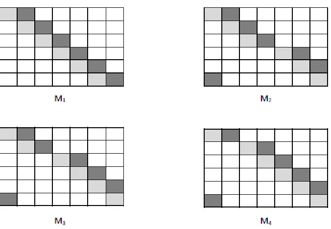
Figure 2 shows the first two edges in the four perfect matchings required for a 4-intersecting Hamiltonian cycle when σ= (a1, a2, . . . , a6),q=r andn= 7. The boxes represent the partsa1 to a6 ordered from top to bottom —Ej,1 is shaded in light grey whileEj,2 is shaded in dark grey, for
1≤j≤4. Each matching has seven distinct edges.
Lemma 4.2. LetH =H(n, r, q|σ) withσ = (a1, a2, . . . , as), s≥2 and∆ =a1 ≥a2≥. . .≥as=
δ≥1. Let 2≤k≤s. If (r+ 1)|q and n≥s+ 1, then H has a k-intersecting Hamiltonian cycle.
Proof. Let us consider the first r+ 1 vertices in V1, . . . , Vn as an (r+ 1)×n grid of vertices. We
construct k matchings M1, . . . , Mk which we then use to construct a k-intersecting Hamiltonian
Figure 2: σ = (a1, a2, . . . , a6) - matchings M1 toM4
The first matching M1 is for the top r vertices in V1 toVn, and is equivalent to the matching
M in Lemma 4.1, with edges labelled asE1,1, E1,2, . . . , E1,n.
In the matching M2 for the (r+ 1)×ngrid , we take edges E2,1 toE2,n so that edge E2,i has
part a1 as in E1,i, but replacing the last vertex in this part with the (r+ 1)th vertex in the same
class, parts a2 toak−1 as in edge E1,i, while partsak toas are as in edge E1,i+1.
In the matching M3, we take edgesE3,1 toE3,n so that edge E3,i has part a1 as in edge E2,i,
partsa2 toak−2 as in edge E1,i, while partsak−1 toas are as in edge E1,i+1.
In general, in the matching Mj, we take edgesEj,1 toEj,n so that edgeEj,i has parts a1 as in
edge E2,i, parts a2 to ak−j+1 as in edge E1,i, while parts ak−j+2 to as are as in edge E1,i+1, for
3≤j≤k.
Now we form a k-intersecting cycle C1 by taking the edges in the following order:
E1,1, E2,1, . . . , Ek,1, E1,2, . . . , Ek,2, . . . , E1,i, E2,i, . . . , Ek,i, E1,i+1, . . . , Ek,i+1, . . . , E1,n, . . . , Ek,n.
We now look at the intersections:
E1,1, E2,1, . . . , Ek,1 intersect ina1−1 vertices in part a1 inV1. E2,1, E3,1, . . . , E1,2 intersect in partsak toas inVk+1 toVs+1. E3,1, E4,1, . . . , E2,2 intersect in partak−1 inVk.
In general,Ej,i, Ej+1,i, . . . , Ej−1,i+1 intersect in partak−j+2 for 3≤j ≤k. The lastk−1 edges
intersectE1,1 in partsaktoasinVktoVs, making this cycle ak-intersecting cycle. Any other sets
of k or more edges will have an empty intersection since they will always include two edges from one matching, which have an empty intersection by definition.
Now ifq ≥r+ 1 and (r+ 1)|q, then for the nextr+ 1 vertices inV1 toVnwe can create another
cycle C2 in the same way. To link C1 and C2, we must consider the last k−1 edges taken in C1,
that is edgeE2,n toEk,n. For edgeE2,n,we change partsak toas and choose them to coincide with
the same parts in the first edge in C2, and in general, for edgeEj,n we change parts ak−j+2 to as
Hence if q=p(r+ 1), we have a k-intersecting Hamiltonian cycle C=C1∪C2∪. . .∪Cp, with
the lastk−1 edges ofCp intersecting the first edge ofC1 by changing the respective parts in these
edges in a similar way as described forC1 intersecting C2.
We can now prove a generalised form of Theorem 3.5:
Theorem 4.3. Let H = H(n, r, q | σ), where s(σ) ≥ 2. For 2 ≤ k ≤ s, if q ≥ r(r −1) and
n≥s+ 1, then H has ak-intersecting Hamiltonian cycle.
Proof. By Theorem 3.4, we know that ifq≥r(r−1), there exist nonnegative integersxandy such that xr+y(r+ 1) =q, since r and r+ 1 are always coprime. So let us divide the q×ngrid into
x consecutive grids of sizer×n, followed by y consecutive grids of size (r+ 1)×n. If we consider thexr×ngrid first, we know that by Lemma 4.1, there is ak-intersecting cycle C1 covering these
vertices, and by Lemma 4.2, there is a k-intersecting cycle C2 covering the y(r+ 1)×n grid. If x= 0 or y= 0, thenC1, respectivelyC2 give the required k-intersecting Hamiltonian cycle. So we
may assume that both x and y are greater than 0. We now need to look at linking C1 toC2 and
vice versa. Firstly, instead of linking the lastk−1 edges inC1 with the first one, we link them to
the first edge in C2, as follows: for edge E2,n,we change parts ak to as and take them to coincide
with the same parts in the first edge in C2, and in general, for edge Ej,n we change parts ak−j+2
toas and take them toncoincide with the same parts in the first edge inC2.
The last k−1 edges ofC2, must be linked to the first edge in C1. So we change the respective
parts in these edges and take them to coincide with the same parts in the first edge in C1, in a
similar way to how we linked the lastk−1 edges inC1 to the first edge in C2. ThusC1∪C2 form
a k-intersecting Hamiltonian cycle in H.
5
Conclusion
The paper [2] definedσ-hypergraphs and started their study in order to investigate what are known as mixed colourings or Voloshin colouring [11] of hypergraphs. In the colourings in [2], no edge was allowed to have all vertices having the same colour, or all vertices having different colours. This study was continued in [3]. These papers demonstrated the versatility of σ-hypergraphs in obtaining interesting results on mixed colourings. In [4], the study ofσ-hypergraphs was extended to two other classical areas of graph and hypergraph theory: matchings and independence. In this paper we continue in this vein, showing that σ-hypergraphs can also give elegant results on Hamiltonicity.
References
[1] Berge, C. Hypergraphs: Combinatorics of Finite Sets volume(45), Elsevier, 1984.
[2] Caro, Y. and Lauri, J. Non-monochromatic non-rainbow colourings ofσ-hypergraphs Discrete Mathematics, 318(0):96–104, 2014.
[3] Caro, Y., Lauri, J. and Zarb, C. Constrained colouring and σ-hypergraphs. Discussiones Mathematicae Graph Theory, accepted, 2014.
[5] Gould, R.J. Recent Advances on the Hamiltonian problem: Survey III. Graphs and Combina-torics, 30(1):1–46, 2014.
[6] Katona, G.Y. Paths and Cycles in Hypergraphs. Presented at Graph Theory Conference in honor of Egawa’s 60th birthday, 2013 , http://www.rs.tus.ac.jp/egawa_60th_birthday/ slide/invited_talk/Gyula_Y._Katona.pdf.
[7] Katona, G.Y. and Kierstead, H.A. Hamiltonian Chains in Hypergraphs. Journal of Graph Theory, 30(3):205–212, 1999.
[8] K¨uhn, D. and Osthus, D. Hamilton Cycles in Graphs and Hypergraphs: an Extremal Perspec-tive. ArXiv e-prints, 2014.
[9] Ruci´nski, A. and ˙Zak, A. Hamilton Saturated Hypergraphs of Essentially Minimum Size. The Electronic Journal of Combinatorics, 20(2):P25, 2013.
[10] Tuza, Z. Steiner Systems and Large non-Hamiltonian Hypergraphs. Le Matematiche., 61(1),2006.