Large Scale Experiments Data Analysis for Estimation of Hydrodynamic Force Coefficients Part 1: Time Domain Analysis

(1)

LARGE SCALE EXPERIMENTS DATA ANALYSIS FOR

ESTIMATION OF HYDRODYNAMIC FORCE COEFFICIENTS

PART 1: TIME DOMAIN ANALYSIS

M. Naghipour

Department of Civil Engineering, Mazandaran University Babol, Iran, [email protected]

(Received: September 8, 2000 – Accepted in Revised Form: January 4, 2001)

Abstract This paper describes various time-domain methods useful for analyzing the experimental data obtained from a circular cylinder force in terms of both wave and current for estimation of the drag and inertia coefficients applicable to the Morison’s equation. An additional approach, weighted least squares method is also introduced. A set of data obtained from experiments on heavily rough-ened circular cylinders in waves and simulated current has been analyzed by all these techniques. The resulting force coefficients are then used to predict the force from separate experiments-results that have not been used in the analysis. The root mean squares error and bias in the estimation of maxi-mum force in each wave cycle is used as a measure of predictive accuracy and as a basis for compar-ing the analysis techniques. It is found that no scompar-ingle method is consistently better under all circum-stances but on average weighted least squares method generally gives the best predictive accuracy by a small margin. The force coefficients obtained by the various methods significantly decrease when current is added to waves.

Key WordsMorison’s Equation, Weighted Least Squares, Drag and Inertia Coefficients, Ocean Waves

ﻜﭼ

ﻴﻴﻴﻴ

ﻩﺪ

ﻳﺍ

ﺎﻘﻣ

ﻦ

ﻪﻟ

ﺎﻬﺷﻭﺭ

ﻱ

ﻒﻠﺘﺨﻣ

ﺭﺩ

ﺘﺳﺍ

ﻱﺍﺮﺑ

ﻪﻛ ﺍﺭ ﻲﻧﺎﻣﺯ

ﻩﺯﻮﺣ

ﻔ

ﺎ

ﺩ

ﻩ

ﺩ

ﺭ

ﺍﺩ

ﺰﻴﻟﺎﻧﺁ

ﺩ

ﻩ

ﺎﻫ

ﺑ

ﺭﻮﻈﻨﻣ

ﻪ

ﻦﻴﻤﺨﺗ

ﺮﺿ

ﻴﻫ ﺐﻳﺍ

ﺭﺪ

ﻣﺎﻨﻳﺩﻭ

ﻜﻴ

ﮒﺭﺩ ﻲ

ﻭ

ﻥﻮﺴﻳﺭﻮﻣ ﻪﻟﺩﺎﻌﻣ ﺭﺩ ﻲﺳﺮﻨﻳﺍ

ﺮﺑ

ﺍ

ﺘﺳ

ﻪﻧﺍﻮ

ﻫ

ﻗﺍﻭ ﻱﺎ

ﻊ

ﺭﺩ

ﺍ

ﻭ ﺝﺍﻮﻣ

ﺎﻧﺎﻳﺮﺟ

ﺕ

`

ﺎﻳﺎﭘ

ﻜﺑ

ﺎ

ﺭ

ﻣ

ﻰ

ﺭ

ﺩﻭ

ﺗ

،

ﺸ

ﻳﺮ

ﺢ

ﺪﻨﻛﻰﻣ

.

ﻋ

ﺯﻭ

ﺕﺎﻌﺑﺮﻣ

ﻞﻗﺍﺪﺣ

ﺵﻭﺭ

،ﻥﺁ

ﺮﺑ

ﻩﻭﻼ

ﻰﻧ

ﺰﻴﻧ

ﻣ

ﺮﻌ

ﻰﻓ

ﻰﻣ

ﮔ

ﺩﺮ

ﺩ

.

ﺍﺩ

ﺩ

ﻩ

ﻯﺎﻫ

ﺑ

ﺪ

ﻣﺁ ﺖﺳ

ﻩﺪ

ﺁ ﺯﺍ

ﺯ

ﺎﻣ

ﻫﺭﺪﻨﻠﻴﺳ ﺮﺑ ﺶﻳ

ﺳﺍ ﻯﺎ

ﻪﻧﺍﻮﺘ

ﺍ

ﻊﻗﺍﻭ ﺮﺑﺯ ﹰﻼﻣﺎﻛ ﺢﻄﺳ ﺎﺑ ﻯ

ﺭﺩ

ﺝﺍﻮﻣﺍ

ﻭ

ﻧﺎﻳﺮﺟ

ﺕﺎ

ﻪﻴﺒﺷ

ﺎﺳ

ﺩﺮﮔ ﺰﻴﻟﺎﻧﺁ ﺎﻬﺷﻭﺭ ﻦﻳﺍ ﻂﺳﻮﺗ ﻩﺪﺷ ﻯﺯ

ﺪﻳ

ﻩ

ﻧﺍ

ﺮﺿ ﺲﭙﺳ ؛ﺪ

ﺍ

ﺪﺑ ﺐﻳ

ﺳ

ﺖ

ﺁ

ﻩﺪﻣ

ﺍ

ﻦﻳﺍ ﺯ

ﺁ

ﻴﻟﺎﻧ

ﺰ

ﺑ

ﺮ

ﻯﺮﺳ ﻚﻳ

ﺩ

ﻩﺩﺍ

ﻫ

ﻪﺘﻓﺮﮔ ﺭﺎﻜﺑ ﺮﮕﻳﺩ ﻯﺎ

ﺷ

ﻩﺪ

ﺪﻧﺍ

.

ﺑ

ﺍﺮ

ﻯ

ﻘﻣ

ﻳﺎ

ﻪﺴ

ﻭﺭ

ﺷ

ﺎﻬ

ﻣ ﻯ

ﺨ

ﻠﺘ

ﻒ

ﺁ

ﻟﺎﻧ

ﺰﻴ

ﺭﺩ

ﺮﻫ

،ﻞﻜﻴﺳ

ﻣ

ﺯﺍ ﺝﻮ

ﺭﺬﺟ

ﺎﻴﻣ

ﺕﺎﻌﺑﺮﻣ ﻦﻴﮕﻧ

(

RMSE

)

ﻭ

ﻴﻣ

ﺎﻧ

ﻴﮕ

ﻦ

ﺧ

ﻝﺎﻣﺮﻧ ﻱﺎﻄ

(

MNE

)

ﺍ

ﺘﺳ

ﺎﻔ

ﻩﺩ

ﻩﺪﺷ

ﺳﺍ

ﺖ

.

ﻣ

ﻼ

ﻈﺣ

ﻪ

ﮔ

ﻲﻤﻧ ﻲﻳﺎﻬﻨﺘﺑ ﻲﺷﻭﺭ ﭻﻴﻫ ﻪﻛ ﺪﻳﺩﺮ

ﺗ

ﻤﺗ ﻦﺘﻓﺮﮔ ﺮﻈﻧ ﺭﺩ ﺎﺑ ،ﺪﻧﺍﻮ

ﺎ

ﻂﻳﺍﺮﺷ ﻡ

،

ﺮﺘﻬﺑ

ﺍ

ﺯ

ﺑﺎﻳﺯﺭﺍ ﻱﺮﮕﻳﺩ

ﻲ

ﮔ

ﺩﺩﺮ

.

ﺎﻣﺍ

ﻱﺭﺍﺪﻘﻣ ﺎﺑ ﻱﺮﺘﺸﻴﺑ ﺖﻗﺩ ﻲﻧﺯﻭ ﺕﺎﻌﺑﺮﻣ ﻞﻗﺍﺪﺣ ﺵﻭﺭ ﻉﻮﻤﺠﻣ ﺭﺩ

ﻲﮔﺪﻨﻛﺍﺮﭘ

ﻲﻣ ﻥﺎﺸﻧ

ﻧ ﻭ ﺪﻫﺩ

ﻼﻣ ﺰﻴ

ﺣ

ﻈ

ﻪ

ﺍ ﻪﺑ ﻥﺎﻳﺮﺟ ﻲﺘﻗﻭ ﻪﻛ ﺪﻳﺩﺮﮔ

ﻲﻣ

ﻪﻓﺎﺿﺍ ﺝﺍﻮﻣ

ﮔ

ﻴﻣﺎﻨﻳﺩﻭﺭﺪﻴﻫ ﺐﻳﺍﺮﺿ ،ﺩﺩﺮ

ﻜ

ﻲ

ﺑ

ﺪ

ﺳ

ﺖ

ﺳﻮﺗ ﻩﺪﻣﺁ

ﻂ

ﺭ

ﻭ

ﺷ

ﻬ

ﺎ

ﻱ

ﺶﻫﺎﻛ ﻲﻬﺟﻮﺗ ﻞﺑﺎﻗ ﺭﻮﻄﺑ ﻒﻠﺘﺨﻣ

ﻲﻣ

ﺑﺎﻳ

ﺪ

.

INTRODUCTION

There has been a considerable volume of ex-perimental research undertaken to estimate the force coefficients in Morison's equation [1]. Much of the early work was undertaken at small scale but the experiments described and discussed in this paper were undertaken in a large 2-D wave flume. Offshore current may augment the wave par-ticle kinematics. In the laboratory this can be

simu-lated either by circulating the water in the wave flume or by attaching the test cylinder to a moving carriage. In the experiments described in this paper the later approach has been used.

(2)

used when estimated the drag and the inertia coefficients (Cd and Cm) for Morison's equation [1].

A variety of procedures have been used to analyze the experimental data in the context of Morison's equation and to predict Cd and Cm. The methods used in time domain analysis are described in third section of this paper.

Sometimes experimenters have justified their choice of analysis on the basis of how well the predicted Morison force compares with the measured force. However as the force coefficients are derived from the measured force one would expect the reconstruction of force time histories to be quite satisfactory, provided that Morison’s equation was a suitable model. This is not an independent test.

By splitting the experimental data from a ran-dom wave experiment into two parts, a more de-manding test can be devised. The first part of the time history is analyzed to obtain predictions for Cd and Cm. These values are then used with parti-cle kinematics measured in the second part to pre-dict the force time series measured in the second part. This provides a more independent assessment of predictive accuracy.

In order to estimate predictive accuracy a measure is needed of how well the predicted force maps onto the independently measured force. One measure would be the root mean squares error normalized by some function of the magnitude of the measured signal. This would measure the quality of the mapping at all points of the time series. However it is the maximum magnitude of the force involving a single extreme wave, which is of interest in the ultimate limit state design assessment.

In the fatigue limit state it is the range of the force produced by each wave, which is of concern, and in particular that produced by the larger waves. In this paper the root mean squares error in the prediction of the maximum and minimum (maximum negative) force normalized by the measured force is used as one measure of predictive accuracy. To avoid the influence of irrelevant small waves only the fit to waves of above average height are con-sidered. The normalized mean bias in this fit is used as the other measure of predictive accuracy.

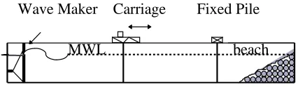
Figure 1. Schematic fixed and mobile cylinders in the large wave flume.

The next section of the paper describes the experiments. The third section describes the various methods for the prediction of force coefficients from experiment data. The fourth section presents the discussion of the results from the analysis of the experiment data. Finally some conclusions are drawn.

DESCRIPTION OF THE EXPERIMENTS

A series of experiments were made to examine the wave loading on two large-scale circular cylinders in the Delft Hydraulic Laboratory’s Delta wave flume in the Netherlands [2].

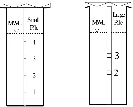
Figures 1 and 2 show a schematic longitudinal section of the flume with a cylinder mounted on the moving carriage, a fixed cylinder, the beach, the wave-maker and the force sleeves’ positions. The details of the six experiment runs consid-ered here are given by [3] from which it can be found that there were experiments with both the small and large cylinders stationary, with a current in the wave direction and a current opposing the wave direction. The currents were achieved by translating the cylinder on the moving carriage away from the wave maker and towards the wave maker respectively.

METHODS FOR ESTIMATING FORCE COEFFICIENTS

There are many methods for estimating force coef-ficients from the data produced from experiments in waves, wave and current and other oscillatory flows. The methods used in time domain analysis are explained briefly. Also the weighted least squares method that has been developed by the author is considered.

(3)

MWL Small Pile 4 3 2 1

Large

MWL

Pile

3

2

Figure 2. Schematic cylinders in the flume with the force sleeves' positions.

Trough-Crest Linear Theory

Fitting One approach to evaluating the hydrodynamics force coefficients is to assume that the velocity and acceleration are 90 degrees out of phase, so when the velocity is maximum, the acceleration is zero and vice versa, thus there are specific locations where the force is purely drag and purely inertial, and Morison's equation can be written at these two points as below and then the coefficients may be easily determined [4].

f

=

K

_D

u

₀2

| sin | sin

Θ

+

K

_M

u

₀

ω

cos

Θ

(1) where

K

D

=

0

5

DC

d

K

M

=

0

25

D

C

m

2

.

ρ

.

ρπ

(2)

Θ = wave phase

where ρ = mass density of water, D is the diameter of the cylinder and

C

_m and C_d are the inertia and drag force coefficients, respectively.

The Fourier Averages

Method Keulegan and Carpenter [5] introduced a method that they used for relatively low Reynolds numbers through measurements on a horizontal cylinder and a sphere in an experiment with standing waves. According to this method, the force applied to a cylinder submerged in waves can be expressed by

considering linear theory described by Equation 1 and the inertia and drag force coefficients can, respectively, be determined over one cycle using Fourier averaging [6].

The method of Fourier averaging has been developed and used by many authors including Bearman et al. [7,8], Bishop [9] and Davies [10]. In the method used by Bearman et al. [7], the Morison's equation is multiplied once by u and then by

u

&

and in each case time averaged over a complete wave cycle. The hydrodynamic coeffi-cients can then be determined from the following equations:

C

fu

D

u

C

f

u

D

u

d

=

m

<

>

<

>

=

<

>

<

>

0 5

0 25

3

2 2

. |

|

.

( )

.

ρ

ρπ

where u and

u

&

are the horizontal components of water particle velocity and acceleration, re-spectively and <> indicates time averaging of the enclosed quantity.

In the method used by Klopman and Kostense, the Morison's equation is multiplied first by u|u||

and then by

u

&

and again time averaged on each occasion over each complete wave cycle to give new equations which can be solved to give the following results:

C

fuu

D u

C

f u

D

u

d

=

m

<

>

< >

=

<

>

< >

| |

.

05

025

4

2 2

ρ

ρπ

(4)

If the assumption is made that u and

u

&

both have zero mean value normal distributions, then:

2 u 2 4 u 4 3

3

u 3

u 8

u < >=σ <& >=σ_&

π σ >=

<| | . (5)

In the case that waves are combined with current, then considering the terms < u& u|u|> <

u

&

u> and

|> u | u u

(4)

C

fu

u

fu

uu

D

u

C

fu

u

fu

uu u

D

u

d

m

=

< ><

> − < >< >

< >< >

=

< >< > − < ><

>

<

>< >

&

.

( | |

&

)

&

| |

&

| |

.

(

&

| |

)

.

. .

. 2

3 2

3

2 2 3

05

025

ρ

ρ π

(6)

and Equation 4 as:

C

fu

u

f

u

D

u

C

f

u

fu

u

D

u

d

m

=

<

><

> − <

><

>

<

><

> − <

>

=

<

><

> − <

><

>

<

><

> − <

>

|

.

(

|

)

|

.

(

|

)

. . .

. .

2

4 2

2

4

2 2

4 2

0

5

0

25

ρ

ρ π

(7)

where u is the horizontal components of water particle velocity when a steady current exists.

Mean Squares

Method The mean squares method derived by Bishop [12] is yet another way to determine hydrodynamic coefficients in time domain analysis.

Bishop [13] has given a brief review of mean squares theory and Shipway. He has obtained the following results applicable to a random sea:

<

>

<

>

=

<

>

<

>

+

F

u

A

u

B

2

2 4

2

&

(8)

in which, <.> denotes the expected value of the random quantity enclosed in the <> estimated from whole time series and F is the mean squares 2 value of the force and

A

=

0 5

.

C

_d

ρ

D

B

=

0 25

.

C

_m

ρ π

D

2 (9)

Davies [10] has discussed the problems of using this method in detail.

Method of Moments Applied to the Force

Time History

Pierson and Holmes [11] have

used moment generating function-derived equations to determine hydrodynamic force coefficients. They assumed that u and

u

&

are independent normal random variables with mean values of zero. Muga and Wilson [14] used this method and found the values of

C

m_and

C

d_{according to the} following equations:

µ

σ

µ

σ

2

2 4 2 2

4

4 8 2 4 2 2 4 4

3

105

18

3

10

=

+

=

+

K

D u M u

D u D u M u M u

&

& &

(

)

In these equations, σ2_u and σ2_u_& are estimated from the experimental data and µ₂ and µ₄ are defined by:

µ

2

µ

2

1

4

1

=

= =

∑

n

i

f

i

and

n

f

n

i i

n

(11)

The coefficients of Equation 10 are obtained from the following definitions:

K

K K

M

u

D

u

M u

u

= −

=

− −

= −

( )

( ) .

. .

µ µ

σ

µ µ µ

σ

µ σ

σ

4 2

2 05

4

2 4 2

2

2 4

2 3

78

3 3

78 3

12

Least Squares Method

One of the most straightforward methods for estimating the coefficients is the least squares method. In this method the coefficients can be estimated by minimizing the sum of the squares of the difference (measured at each small time interval) between the time series of the measured and predicted forces. This method can be used either for each individual wave cycle, defined between successive zero up-crossings or for whole wave records (i.e. about 20 minutes of data).

Correspondingly, it is assumed that C_m and

d

(5)

C

fu u

u

f u

u u u

D

u

uu u

C

f u

u

fu u

uu u

D

u

uu u

d

m

=

−

=

−

∑

∑ ∑

∑

∑ ∑

∑

∑ ∑

∑

| |

.

(

| |) )

( )

| |

.

(

| |) )

. . .

. .

2

4 2

2

4

2

4 2

0 5

13

0 25

ρ

ρ π

If we consider the waves to be linear and use the data from a single whole wave cycle, then:

∑

u u u

| |

=

.

0

(14)

and Equation 16 are simplified to:

C fu u

D u C

f u

D u

d = m=

∑

| |

. ( )

.

0 5

0 25

4

2 2

ρ _ρπ (15)

This method was developed by [15] He showed that depending on the wave and cylinder character-istics, data can be well or poorly-conditioned for resolving

C

_d and

C

_m. He presented a criterion for evaluating the suitability of data for determining

C

m and

C

d as "reliability ratio"

R

D u u

= < >

< >

2 4

2

π .

(16)

Dean [15] suggested that data will be well-conditioned for evaluating both

C

m and

C

d to-gether when 0.25<R<4 and for

C

_m only when

0<R<0.25 and for

C

_d only when R>4

Weighted Least Squares Method

A weighted least squares analysis, which has been in-troduced by [3] can also be applied to the data. Us-ing such an approach the author has found a no-ticeable reduction is achieved in the error between fitted and measured values at the peaks of the force time series for waves with heights of more than the root-mean-squares wave height (H>H_rms). This approach may have a significant affect when extreme value and peak-to-peak range of Morison

force are required. This is the case for estimating extreme collapse loading and fatigue loading re-spectively of offshore jacket structures. The weighted least squares formulation is:

e

f

DC u u

D C u

e f

f

E

N

e f

E

C

E

C

f e d m

f

k k

e f

k

m d

= −

+

=

−

=

∑

( .

| | .

)

(

)

(

)

.

05

0 25

1

0

17

2

2 2

ρ

ρ π

∂

where k is an arbitrary positive number and the terms

e

_f

,

f

_e

,

E

,

N

define the error of the es-timated force, the eses-timated force, mean squares error and number of data from which the coeffi-cients are evaluated respectively. The parameter k

is considered as a constant that can be selected to minimize the error in the critical peak force areas. The coefficients are then obtained as below:

(18) All the parameters in these equations are defined above. It has been found that the constant the k can be optimized in an iterative manner to give a minimum predictive error in the peak force re-gions.

DISCUSSION OF RESULTS

The principal objective of this paper is to examine the efficiency of the various methods of analysis rather than to present a very extensive set of

C

f

fu

u

f

u

f

u

f

u

D

f

u

f

u

f

u

C

f

u

f

u

f

fu

u

f

u

D

f

u

f

u

f

u

d

k k k k

k k k

m

k k k k

k k k

=

−

=

−

∑

2 2

2

2 2

2 4 2

2

2 2

2 2 4 2 2

2 2

2

2 4 2 2

0

5

4

|

.

(

|

)

|

(

|

)

. . .

. .

ρ

(6)

experimental data and so only a subset of a larger project is considered. The experiments considered here all had heavy (artificial marine) roughness on them. The results of the other experiments in the same project, on smooth cylinders and those with slight roughness are presented in Mackwood, et al. [16].

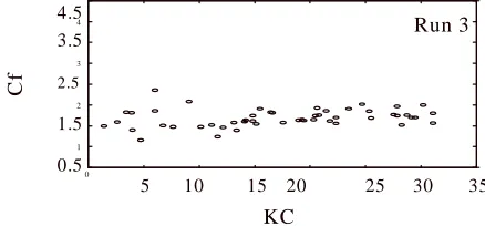
Effect of Keulegan Carpenter Number

Before examining the efficiency of the various methods for estimating Cd and Cm from random wave data it is interesting to look at plots of Cf against KC (Cf is a root mean squares force coefficient); s e e B e a r ma n , e t a l . [ 7 ] ,

Cf

f

Du

rms

=

0 5

.

ρ

2

where

f

rms is root mean squares value of in-line force,

u

rmsis root mean squares value of horizontal water particle velocity, D is the diameter of the cylinder and

ρ

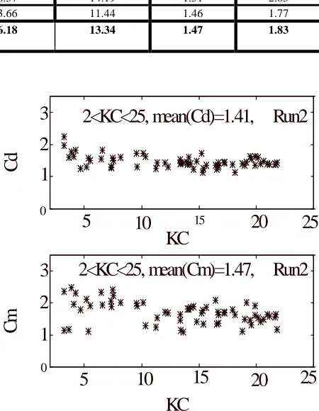
is mass density of water. The re-sults obtained with no current are shown in Figure 3 for the large cylinder. These results have been obtained by analyzing each wave in the random wave train separately. Figure 4 shows that the ef-fect of introducing a positive current is to reduce not only the scatter in Cf at low KC values but also its average magnitude. A negative current reduces the average magnitude even further and across a wider range of KC as can be seen in Figure 5. The inference that can be drawn is that at low KC with-out current a large number of correspondingly small waves are needed to estimate a mean value of Cf, and also Cd and Cm, with statistical accu-racy.

This variation in scatter with KC is also seen in some cases after the total force is split into drag and inertia components as can be seen in Figure 6. Here Cd and Cm have been estimated using the wave-by-wave least squares method (WWLSM). Interestingly for the larger pile in the no current condition the Cd shows most of the scatter at low KC and Cm has lower scatter, which is apparently

independent of KC, as is seen in Figure 6. For the smaller pile on the other hand the scatter in both Cd and Cm is similar. This is reflected in Dean's "reliability coefficient" R (Figures 7 and 8). In all cases there is at least some tendency for the scatter to reduce as the KC in creases but there is very lit-tle variation in the average value of either Cd or Cm above a KC of around 7 for both the with and

0

2 4 6 8 10 12 14

0

20 40 60 80 100

Cf

Run 1

KC

Figure 3. Variation of Cf with KC in the random waves (fixed large pile).

0

5 10 15 20 25

0.5

1

1.5

2

2.5

3

3.5

4

4.5

KC

Cf

Run 2

Figure 4. Variation of Cf with KC in the random waves (mo-bile large pile, = +1m/sec).

0

5 10 15 20 25 30 35

0.5 1 1.5 2

2.5

3 3.5 4 4.5

KC

Cf

Run 3

(7)

without current cases. Because of this average re-sults for Cd and Cm are considered hereafter in this paper.

Assessing Predictive Accuracy

In a statistical sense a good estimator should be unbiased and of minimum variance. This is equally important when estimating the forces on offshore structures and in this paper two corresponding parameters are used to assess how well a predicted force time series compares with the corresponding measured force time series. These parameters are the mean nor-malised error (MNE) and root mean squares error (RMSE) are given by:

MNE

N

f

RMSE

N

f

m i e i

m i i

N

m i e i

m i i

N

=

−

=



−











=

∑

100

1

2

(

)

( )

(

)

(

)

( )

(

)

(19)

where

f

_m is maximum of absolute value of meas-ured force,

f

e is the same as

f

m but for predicted force and N is the number of waves of above aver-age height. These parameters provide a basis for comparing force coefficients obtained by the dif-ferent analysis methods discussed earlier. They are also used to compare measured wave particle ve-locity and those predicted by wave theories from surface wave height and period.

The parameters above can be unduly influenced when

f

m is small and the absolute error is large so it is desirable not to consider small waves and their corresponding forces when predicting the meas-ured time series. For jacket type offshore struc-tures, the ultimate wave loading involves very high KC and most of the fatigue damage occurs in waves of at least moderate KC (typically above about 7-10). Therefore, it was decided to see how well the measured force due to waves of above av-erage height could be predicted.

Figure 6. Variation of reliability ratio with KC for fixed large pile.

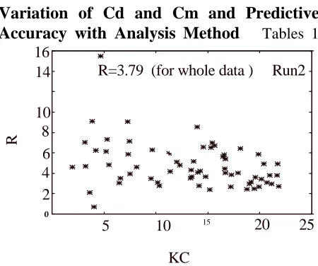
Figure 7.Variation of Cd and Cm with KC in the random waves for a fixed large pile (using wave by wave least square method (WWLSM).

Variation of Cd and Cm and Predictive

Accuracy with Analysis Method

Tables 1

0

2 4 6 8 1 0 1 2 1 4 1 6

0 0 .5 1 1 .5

K C

R

0

5 10 15 ₂₀ ₂₅

0

2 4 6 8 10 14 16

KC

R

R=3.79 (for whole data ) Run2

Figure 8. Variation of reliability ratio with KC for mobile large pile.

0 2 4 6 8 10 12 14 16

0 2 4 6

KC

Cd

1<KC<18, mean(KC)=5.5, mean(Cd)=1.61, Run 1

0 2 4 6 8 10 12 14 16

0 1 2 3

KC

(8)

curacy with Analysis Method

Tables 1 and 2 show the mean values of Cd and Cm obtained us-ing the various analysis methods described in Sec-tion 3. For those methods, which use a wave-by-wave analysis, a pair of force coefficients is ob-tained for each wave cycle and in these cases the standard deviations are quoted. Also shown in these tables are the corresponding mean bias and standard error when these coefficients are used for predicting the second, unanalyzed, part of the measured force time series.

Looking at the wave by wave analysis methods in these tables it is noticeable that the standard de-viation of the Cd values reduce significantly in all cases with the addition of current but for the Cm values the reverse is true. When it comes to predic-tive accuracy few clear trends occur. The rmse tends to reduce somewhat in most cases when cur-rent is added but the bias shows no particular trend. As far as the analysis methods are con-cerned the performance are quite similar as would be expected in light of the similarity among these methods shown in Section 3. For these data sets the least squares method comes out slightly ahead overall of the existing methods for wave-by-wave analysis but not consistently so. The weighted least squares (particularly with a weight index of 2) is seen to be generally superior to the existing methods.

The method of moments applied to the whole time history of each run gives results with gener-ally low bias, less than 8%, and rmse values of 9.5 to 15 %.

The least squares method applied to the whole time history has a bias of less than 9% for all the runs an average of less than 4%. The correspond-ing rmse varies between 7.5 and 16% and the method seems to give force coefficients broadly consistent with other methods. The author has tried a weighted least squares approach as de-scribed in section 3.6 and by Equations 17 and 18, which gives additional emphasis to the fitting at large values of the modules of the measured force. The results show some improvement when this is done and the bias is always less than 6.3% with an average of 2.03% for a power factor of n=2 but the rmse still varies from 7.36 to 14.79%.

Table 3 shows the averages from all the meth-ods discussed above used for each run together with the overall averages for all six runs. Overall the mean value of Cd is 1.47 and Cm is 1.83 with an overall average rmse of 13.34% and mean mod-ules of bias of 6.18.

CONCLUSIONS

It is clear that the method used to analyze experiment

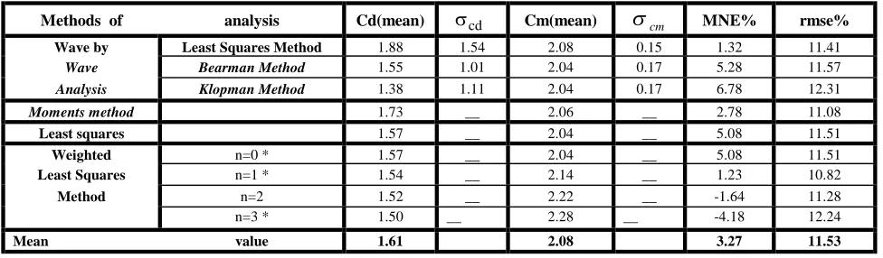
TABLE 1. Values of

C

_m and

C

_d from the Analysis Methods in the Random Waves for a Fixed Large Pile (* :The Result is not Included in the Mean Value).

Methods of analysis Cd(mean) σ_cd Cm(mean)

σ

_cm MNE% rmse%

Wave by Least SquaresMethod 1.88 1.54 2.08 0.15 1.32 11.41

Wave Bearman Method 1.55 1.01 2.04 0.17 5.28 11.57

Analysis Klopman Method 1.38 1.11 2.04 0.17 6.78 12.31

Moments method 1.73 __ 2.06 __ 2.78 11.08

Least squares 1.57 __ 2.04 __ 5.08 11.51

Weighted n=0 * 1.57 __ 2.04 __ 5.08 11.51

Least Squares n=1 * 1.54 __ 2.14 __ 1.23 10.82

Method n=2 1.52 __ 2.22 __ -1.64 11.28

n=3 * 1.50 __ 2.28 __ -4.18 12.24

(9)

TABLE 2. Values of

C

_m and

C

_d from the Analysis Methods in the Random Waves for a Mobile Large Pile (* :The Result is not Included in the Mean Value).

TABLE 3. Values of

C

_m and

C

_d from the Analysis Methods in the Random Waves (Averaged in the Six Runs).

data in terms of Morison equation has a significant affect on both the force coefficients obtained and their predictive accuracy. It is found that no single method is consistently better under all circumstances but on average the wave by wave weighted least squares method gives both the lowest bias (2.03%) and root mean squares error (10.9%) as can be seen in Table 3.

The force coefficients obtained by the various methods varied significantly but there was a clear trend which showed that the addition of current significantly decreased the drag coefficient and to a lesser extent the inertia coefficient.

For KC values of above around 10, uses of sin-gle mean drag and inertia coefficients (about 1.7 and 2, respectively) for heavily marine roughened cylinders in waves without current, seems satisfac-tory. When current is present, both coefficients should be significantly less than the above values (see Figures 8 and 9 and Table 2).

M e t h o d s o f A n a l y s i s Cd(mean)

σ

cdCm

Cm(me a n)

σ

cm M N E

%

r m s e

%

W a v e b y L e a s t S q u a r e s M e t h o d 1 . 5 1 0 . 3 7 1 . 7 2 0 . 7 2 2 . 8 2 8 . 4 4

W a v e B e a r m a n M e t h o d 1 . 3 2 0 . 3 7 1 . 4 9 0 . 5 6 1 5 . 1 8 1 6 . 6 9

A n a l y s i s K l o p m a n M e t h o d 1 . 3 2 0 . 3 6 1 . 5 0 0 . 5 7 1 5 . 5 4 1 7 . 0 1

M o m e n t s M e t h o d 1 . 4 6 _ _ 0 . 5 3 _ _ 7 . 8 0 1 1 . 0 1

L e a s t S q u a r e s 1 . 4 2 _ _ 1 . 5 9 _ _ 8 . 7 4 1 1 . 5 0

W e i g h t e d n = 0 * 1 . 4 2 _ _ 1 . 5 9 _ _ 8 . 7 4 1 1 . 5 0

L e a s t S q u a r e s n = 1 * 1 . 4 4 _ _ 1 . 8 2 _ _ 7 . 2 9 1 0 . 4 9

M e t h o d n = 2 1 . 4 4 _ _ 1 . 9 8 _ _ 6 . 2 6 9 . 8 5 n = 3 * 1 . 4 5 _ _ 2 . 1 3 _ _ 5 . 3 6 9 . 3 5

M e a n V a l u e 1 . 4 1 1 . 4 7 9 . 3 9 1 2 . 4 2

Methods of Analysis %Bias %RMSE Cd(mean) Cm(mean)

Time Domain Least SquaresMethod 5.56 12.83 1.42 1.80

( Wave by Bearman Method 10.19 15.76 1.49 1.65

Wave Klopman Method 9.09 14.91 1.44 1.66

Analysis) WLSM (2) 2.03 10.90 1.51 2.04

Moments Method 6.57 14.19 1.51 2.05

Least Squares 3.66 11.44 1.46 1.77

Mean

Value 6.18 13.34 1.47 1.83

5

10

15

20

25

0

1

2

3

KC

Cm

2<KC<25, mean(Cm)=1.47, Run2

5

10

15

20

25

0

1

2

3

KC

Cd

2<KC<25, mean(Cd)=1.41, Run2

(10)

REFERENCES

1. Morison, J. R., O'brien, M. P., Johnson, J. W., and Schaaf, S., “The Force Exerted by Surface Wave on Piles”,Transactions of the American Institute of Min-ing and Metallurgical Engineers, Vol. 189, (1950), 147-154.

2. Wolfram, J. and Naghipour, M., “On the Estimation of Morison Force Coefficients and Their Predictive Accu-racy for Very Rough Circular Cylinders”,Applied Ocean Research, 21, (1999), 311-328.

3. Naghipour, M., “The Accuracy of Hydrodynamic Force Prediction for Offshore Structures and Morison's Equa-tion”,Thesis Submitted for PhD, Heriot-Watt University, Edinburgh

,

(1996).

4. Evans, D. J., “Analysis of Wave Force Data”, Offshore Technology Conference, Paper Number OTC 1005, (1969).

5. Keulegan, G. H, and Carpenter, L. H., “Forces on Cylin-ders and Plates in an Oscillating Fluid”, Journal of Re-search of the National Bureau of Standards, Vol. 60,5, (1958), 423-440.

6. Chakrabarti, S. K., “Hydrodynamics of Offshore Struc-tures”, Computational Mechanics Publications, New York, (1987).

7. Bearman, P. W., Chaplin, J. R., Graham, J. M. R., Kos-tense, J. K., Hall, P. F., and Klopman, G., “The Loading on a Cylinder in Post-Critical Flow Beneath Periodic and Random Waves”, Behaviour of Offshore Structures,

(1985), 213-225.

8. Bearman, P. W., “Wave Loading Experiments on Circular Cylinders at Large Scale”, Proc. 5th Int. Conf.

OnBehaviour of Offshore Structures, Trondhein, Nor-way, Tapir, (1988) 471-487.

9. Bishop, J. R., “The Mean Square Value of Wave Force Based on the Morison's Equation”, NMI R 40, also OT R-, (1978).

10. Davies, M. J. S., “Wave Loading Data from Fixed Verti-cal Cylinders”, OTI 92 558, 89, (1993).

11. Pierson, W. J. and Holmes, P., “Irregular Wave Forces on a Pile”, J. of the Waterways and Harbours Div., Proc. of the American Society of Civil Engineers (ASCE), Vol. 91, No. WW4, (1965), 1-10.

12. Bishop, J. R., “Wave Force Investigation at the Second Christchurch Bay Tower, Summary Report”, NMI R177, OT-O-82100

, (1984).

13. Bishop, J. R., and Shipway, J. C., “Wave Force Coeffi-cients from the Second Christchurch Bay Tower”

,

NMI R 178, also OT-O-82101 Part 1, (1984).

14. Muga, B. J., and Wilson, J. F., “Statistical Approach to the Evaluation of Inertial and Drag Coefficients for Sin-gle Members”, Dynamic Analysis of Ocean Structures,

(1970), 134-150.

15. Dean, R. G., “Methodology for Evaluating Suitability of Wave and Wave Force Data for Determining Drag and Inertia Coefficients”, Proc. 1st Int. Conf. on Behaviour of Offshore Structures,Trondheim, Norway, (1976), 40-64.