Development of an Implicit Numerical Model for Calculation of Sub and Super Critical Flows

DEVELOPMENT OF AN IMPLICIT NUMERICAL MODEL FOR

CALCULATION OF SUB- AND SUPER-CRITICAL FLOWS

M.R. Hadian, A.R. Zarrati and M. Eftekhari

Department of Civil and Environmental Engineering, Amirkabir University of Technology No. 424, Hafez Avenue, 15914, Tehran, Iran

[email protected] - [email protected]

(Received: January 31, 2004 – Accepted: February 24, 2005)

Abstract A two dimensional numerical model of shallow water equations was developed to calculate sub and super-critical open channel flows. Utilizing an implicit scheme the steady state equations were discretized based on control volume method. Collocated grid arrangement was applied with a SIMPLEC like algorithm for depth-velocity coupling. Power law scheme was used for discretization of convection and diffusion terms. Under relaxation factors were introduced in the model to prevent divergence. Momentum interpolation was used in calculating velocities on cell faces to avoid checker board water surface fluctuation in the collocated grid. The model was verified in different cases including complex water surface profiles and hydraulic jump. The results are compared with experimental and analytical data and the necessary values of under relaxation factors for a converged solution are discussed. No artificial viscosity was required, which is the advantage of the present model.

Key Words Shallow-Water, Under-Relaxation, Sub-critical, Super-critical, Implicit, Numerical Model

ﻩﺪﻴﻜﭼ

ﻢﻛ ﻱﺎﻬﺑﺁ ﺕﻻﺩﺎﻌﻣ ﻞﺣ ﻱﺍﺮﺑ ﻱﺩﺪﻋ ﻝﺪﻣ ﻚﻳ ﺮﺿﺎﺣ ﻪﻟﺎﻘﻣ ﺭﺩ ﻱﺎﻬﻧﺎﻳﺮﺟﺭﺩ ﻩﺩﺎﻔﺘﺳﺍ ﻞﺑﺎﻗ ﻖﻤﻋ

ﻕﻮﻓﻭﻲﻧﺍﺮﺤﺑﺮﻳﺯ ﻪﺋﺍﺭﺍﻲﻧﺍﺮﺤﺑ

ﻩﺪﺷ

ﺖﺳﺍ

.

ﺯﺍﻩﺩﺎﻔﺘﺳﺍﺎﺑﻭﺭﺎﮔﺪﻧﺎﻣﺖﻟﺎﺣﺭﺩﺍﺭﺕﻻﺩﺎﻌﻣﻭﻩﺩﻮﺑﻲﻨﻤﺿﻝﺪﻣﻦﻳﺍ

ﻪﻜﺒﺷﺭﺩﻲﻨﻤﺿﺵﻭﺭﻚﻳ

ﺎﺠﺑﺎﺟﻱﺍ

ﻲﻣﻞﺣﻩﺪﺸﻧ ﺪﻨﻛ

.

ﻪﺑﺎﺸﻣﻲﺷﻭﺭ

SIMPLEC

ﺭﺩﺖﻋﺮﺳﻭﻖﻤﻋﻁﺎﺒﺗﺭﺍﻱﺍﺮﺑ

ﺖﺳﺍﻩﺪﺷﻪﺘﻓﺮﮔﺭﺎﻜﺑﻝﺎﻘﺘﻧﺍﺕﺍﺭﺎﺒﻋﻱﺯﺎﺳﻞﺼﻔﻨﻣ ﻱﺍﺮﺑﺰﻴﻧﻲﻧﺍﻮﺗﻥﻮﻧﺎﻗﺵﻭﺭﻭﻩﺪﺷﻩﺩﺎﻔﺘﺳﺍﺮﺿﺎﺣﻝﺪﻣ

.

ﻝﺪﻣ

ﺢﻄﺳﺕﺎﻧﺎﺳﻮﻧ ﺯﺍﻱﺮﻴﮔﻮﻠﺟﻱﺍﺮﺑﺮﺿﺎﺣ ﺎﺠﺑﺎﺟﻪﻜﺒﺷﺎﺑﻁﺎﺒﺗﺭﺍﺭﺩﺏﺁ

ﻲﻣﺩﻮﺳﻡﻮﺘﻨﻤﻣﻲﺑﺎﻴﻧﺎﻴﻣﺯﺍﻩﺪﺸﻧ ﺪﻳﻮﺟ

.

ﺍﺮﺿ ﻳ ﮕﻤﻫﺩﺎﺠﻳﺍﻱﺍﺮﺑﻒﻴﻔﺨﺗﺮﻳﺯﺐ ﺭﺎﻜﺑﻝﺪﻣﺭﺩﻲﺋﺍﺮ

ﺖﺳﺍﻪﺘﻓﺭ

.

ﻞﻣﺎﺷﻲﻔﻠﺘﺨﻣﻂﻳﺍﺮﺷﺭﺩﻪﺘﻓﺎﻳﻪﻌﺳﻮﺗ ﻝﺪﻣ

ﻞﻴﻓﻭﺮﭘ ﺭﺎﻜﺑﻲﻜﻴﻟﻭﺭﺪﻴﻫﺵﺮﭘﻭﻝﺎﻧﺎﻛﻚﻳﻝﻮﻃﺭﺩﻲﻧﺍﺮﺤﺑﺮﻳﺯﻭﻲﻧﺍﺮﺤﺑﻕﻮﻓﻱﺎﻫ ﺕﺎﻋﻼﻃﺍﺎﺑﻥﺁﺞﻳﺎﺘﻧﻭﻪﺘﻓﺭ

ﺖﺳﺍﻩﺪﺷﻪﺴﻳﺎﻘﻣﻲﻠﻴﻠﺤﺗﻭﻲﻫﺎﮕﺸﻳﺎﻣﺯﺁ

.

ﻥﺎﺸﻧﺞﻳﺎﺘﻧﻪﺴﻳﺎﻘﻣ

ﻲﻣﺮﺿﺎﺣﻝﺪﻣﺭﺎﻛﺖﺤﺻﻩﺪﻨﻫﺩ ﺪﺷﺎﺑ

.

ﻪﺟﻮﺗﺎﺑ ﻪﺑ

ﻲﻨﻤﺿ ﺮﺿﺎﺣﻝﺪﻣﻥﺩﻮﺑ ،

ﺩﺭﺍﺪﻧﺩﻮﺟﻭﺞﻳﺎﺘﻧﻲﺋﺍﺮﮕﻤﻫﻱﺍﺮﺑﻲﻋﻮﻨﺼﻣﺖﺟﺰﻟﺯﺍﻩﺩﺎﻔﺘﺳﺍﻪﺑﻱﺯﺎﻴﻧ

.

ﺖﺴﻴﻟﺎﺣﺭﺩﻦﻳﺍ

ﺍﺮﮕﻤﻫﻱﺍﺮﺑﻲﻋﻮﻨﺼﻣﺖﺟﺰﻟﻝﺎﻤﻋﺍﻪﺑﺯﺎﻴﻧﺢﻳﺮﺻﻱﺎﻬﻟﺪﻣﻪﻛ ﻳ

ﺪﻧﺭﺍﺩﻲ

.

1. INTRODUCTION

The rapid expansion in available computer power has led to increasingly use of computational fluid dynamics (CFD) in fluid-flow problems. Flows in the nature have three-dimensional structures and are usually turbulent. In many cases the geometry of the flow boundaries is also very complex. Solving the equations of motion in these conditions is very difficult. However, in rivers and open channels where the width of the flow is large compared with its depth, the vertical acceleration of water is negligible compared to the gravitational

acceleration. In this condition the equations of motion can be integrated in depth to derive two dimensional depth averaged equations. Although this model may not be very accurate in regions with sharp gradients of water surface profile and strong secondary flows, but it is accurate enough for many practical purposes.

and Mahesawaran [5], Molls and Chaudhry [6], Ye and McCorquodale [7], Klonidis and Soulis [8] and Weerakoon et al. [9] can be mentioned.

The difference in physical property of sub- and super-critical flows and consequently their different numerical treatment caused that most of the computer codes tackle only one of these two flow regimes. Development of a scheme which could simultaneously simulate both sub- and super-critical flows at different parts of the channel is not easy [10]. Some numerical schemes have been developed to simulate such a mixed flow regimes using one or two dimensional models. In one dimensional models, shallow water equations have been used to simulate the mixed flows and hydraulic jump since the early works of Bidone [11]. A rather complete review of these models has been mentioned by Gharangik and Chaudhry [12]. These researchers applied MacCormack and Dissipative Two-Four explicit schemes with the aid of an artificial viscosity to simulate the hydraulic jump. Chaudhty [13] explained some other schemes for capturing such a mixed flow in one dimension, among them, Lambda, Gabutti and different forms of Beam and Warming can be listed here. Recently, Meselhe et al. [14] developed a numerical model by introducing adaptive artificial viscosity to Saint Venant equations too. In this method the artificial viscosity have effective influence on nodes with sharp depth gradient but is suppressed at moderate depth gradients. In two dimensional models, Younus and Chaudhry [15] and Molls and Chaudhry [6] simulated mixed flows, however in these works also artificial viscosity was necessary for convergence of the model. Therefore it can be seen that the use of artificial viscosity is necessary for the above mentioned models which introduces additional uncertainty and acts like a damping factor. Zhou and Stansby [16] developed a 2D shallow water model with an implicit scheme and staggered grid to simulate the hydraulic jump. They showed that no artificial viscosity is necessary in their model for calculating such a mixed flow.

The main objective of the present study is to develop a depth averaged model which is able to calculate combination of sub- and super-critical flows along a channel. The 2D depth averaged shallow water equations were solved by a collocated variable arrangement and depth

correction scheme using a SIMPLEC like algorithm. The applicability of the model in simulation of mixed flows and necessary under relaxation factors is presented here with the aid of few examples.

2. GOVERNING EQUATIONS

Neglecting the wind shear stress, Coriolis acceleration, and using Boussinesq approximation for Reynolds stresses, the conservative form of shallow water equations in steady state can be written as [3]:

( ) ( )

=

₀

∂

∂

+

∂

∂

y

vh

x

uh

(1)

( ) ( )

ρ

τ

ζ

_bx

x

gh

y

vuh

x

uuh

−

∂

∂

−

=

∂

∂

+

∂

∂

⎟⎟

⎠

⎞

⎜⎜

⎝

⎛

∂

∂

∂

∂

+

⎟

⎠

⎞

⎜

⎝

⎛

∂

∂

∂

∂

+

y

u

h

y

x

u

h

x

ν

t

ν

t (2)

( ) ( )

ρ

τ

ζ

by

y

gh

y

vvh

x

uvh

−

∂

∂

−

=

∂

∂

+

∂

∂

⎟⎟

⎠

⎞

⎜⎜

⎝

⎛

∂

∂

∂

∂

+

⎟

⎠

⎞

⎜

⎝

⎛

∂

∂

∂

∂

+

y

v

h

y

x

v

h

x

ν

t

ν

t (3)

In which, u and v are depth averaged velocities in x and y directions respectively (Figure 1), h= water depth, ρ=water density,

ν

_t= depth averaged turbulent viscosity, g=gravitational acceleration,

ζ=water surface elevation (

ζ

=

h

+

Z

_b),

Z

_b=bed elevation,

τ

_bx and

τ

_by=bed shear stresses in x and y directions. These stresses can be calculated from Manning’s equation as:

3 1

2 2 2

h

v

u

u

n

g

bx

=

+

ρ

τ

3 1 2 2 2

h

v

u

v

n

g

by

=

+

ρ

τ

(5)

The depth averaged turbulent viscosity can be calculated by zero-equation models in the following form, especially if there is no re-circulation zone [17].

h

u

t *

6

κ

ν

=

(6)

in which u_*= bed shear velocity and κ is the von Karman constant (= 0.4).

3. NUMERICAL TREATMENT

3.1. Discretization of the Governing

Equations

Based on control volume method the

momentum equation in x and y directions can be descritized following Patankar [18]. Using the power-law scheme for convection and diffusion terms and an under relaxation factor to avoid divergence, the u-momentum equations can be expressed as: u u S N u N a S u S a W u W a E u E a P u u P

a _{= + + + +}

α

(7)

where the coefficients and linearized source terms are:

( )

( )

u x

{

( )

uh y

}

x y h a e e t e e t

E + − ∆

⎪⎭ ⎪ ⎬ ⎫ ⎪⎩ ⎪ ⎨ ⎧ ⎟⎟ ⎠ ⎞ ⎜⎜ ⎝ ⎛ ∆ − ∆ ∆

= max 0, 1 0.1 max0,

5

ν ν

(8)

( )

( )

u x

{

( )

uh y

}

x y h a w w t w w t

W + − ∆

⎪⎭ ⎪ ⎬ ⎫ ⎪⎩ ⎪ ⎨ ⎧ ⎟⎟ ⎠ ⎞ ⎜⎜ ⎝ ⎛ ∆ − ∆ ∆

= max 0, 1 0.1 max0,

5

ν ν

(9)

( )

( )

v y

{

( )

vh x

}

y x h a n n t n n t

N + − ∆

⎪⎭ ⎪ ⎬ ⎫ ⎪⎩ ⎪ ⎨ ⎧ ⎟⎟ ⎠ ⎞ ⎜⎜ ⎝ ⎛ ∆ − ∆ ∆

= max 0, 1 0.1 max 0,

5

ν ν

(10)

( )

( )

v y

{

( )

vh x

}

y x h a _s s t s s t

S + − ∆

⎪⎭ ⎪ ⎬ ⎫ ⎪⎩ ⎪ ⎨ ⎧ ⎟⎟ ⎠ ⎞ ⎜⎜ ⎝ ⎛ ∆ − ∆ ∆

= max 0, 1 0.1 max0,

5 ν ν (11)

(

)

y x u y x h g S p u u w e u

u ∆ ∆

− + ∆ ∆ − −

= 1 *

α α ζ ζ (12) p N S W E

P

a

a

a

a

S

a

=

+

+

+

−

(13)

y x h v u n g

S_p =− + ∆ ∆

3 1 2 2 2 (14)

in which

∆

x

and

∆

y

are dimensions of control volume in x and y direction respectively,

α

_uis the under-relaxation factor for u-momentum and

u

*is the value of velocity from the last iteration. By the same method, the equations for the v-momentum can be written in the following form:

u v N N S S W W E E P v

P _{v a v a v a v a v S}

a + + + + =

α

(15)

in which

α

_vis the under-relaxation factor for v-momentum and the source term defines as:

(

)

x

v

x

y

y

h

g

S

_p v v s n u

v

∆

∆

−

+

∆

∆

−

−

=

1

*

α

α

ζ

ζ

where _v * _{is the value of velocity from the last} iteration.

The values of u and v can, therefore, be calculated from (6) and (14). However the continuity equation can not be used directly for calculating the water surface elevation. Therefore, an equation should be derived for calculation of water surface elevation.

3.2. Velocity-Water Surface Elevation

Coupling

If the values of velocity components and water surface elevation found from the last iteration are shown by an asterisk sign, one can write:

'

and

'

,'

* *

*

+

=

+

ζ

=

ζ

+

ζ

=

u

u

v

v

v

u

(17) where prime shows the correction required for

obtaining the correct values. In the process of iteration, (7) is written as:

− +

+ +

=

αP_u u*p aEu*E aWu*W aSuS* aNu*N

a u u S y x * w * e h g + ∆ ∆ ⎟ ⎠ ⎞ ⎜ ⎝ ⎛_{ζ −ζ}

(18) Subtracting (7) from (18) and neglecting the

second order terms of

ζ

' [17,19] results:

− + + + = α ' N u N a ' S u S a ' W u W a ' E u E a ' p u u u p a y x w ' e ' h g ∆ ∆ ⎟ ⎠ ⎞ ⎜ ⎝ ⎛_{ζ −ζ}

(19) Following the SIMPLEC algorithm [18] one can

write: x ζ B x ζ a α a ∆y ∆x h g u U u nb u u p p _∂ ′ ∂ = ∂ ′ ∂ − − = ′

∑

(20)

In the same way for velocityof v,

y

ζ

B

y

ζ

a

α

a

∆

y

∆

x

h

-g

v

V v nb v v p p

∂

′

∂

=

∂

′

∂

−

=

′

∑

(21)

Discretizing the continuity equation by the same method as momentum equation results in:

(

uh

∆

y

) (

_e

−

uh

∆

y

) (

_w

+

vh

∆

x

) (

_n

−

vh

∆

x

)

_s

=

0

(22) Combining (17) and (22), considering (20) and (21) yields: p S S N N W W E E P

P

ζ

A

ζ

A

ζ

A

ζ

A

ζ

m

A

′

=

′

+

′

+

′

+

′

+

(23)

where e U E ∆x ∆y h B A _⎟⎟ ⎠ ⎞ ⎜⎜ ⎝ ⎛ = , w U W ∆x ∆y h B A _⎟⎟ ⎠ ⎞ ⎜⎜ ⎝ ⎛ = , n V

N _∆y

∆x h B A _⎟⎟ ⎠ ⎞ ⎜⎜ ⎝ ⎛ = , s V

S _∆y

∆x h B A _⎟⎟ ⎠ ⎞ ⎜⎜ ⎝ ⎛

= (24)

(

) (

) (

) (

*

)s

n * w * e *

P u h∆y u h∆y v h∆x v h∆x

m = − + − (25)

where mpis the difference between the discharge

getting out of each cell with what gets into it. At the converged solution mp should become zero and

therefore it can be used as one of the criteria for the convergence.

3.3. Momentum interpolation

To avoid

+ α α α − + = =

∑

v v P a * p v v v 1 S , N , W , E nb nb v v nb a P v y v C 2 K y v v P a y x h g ∂ ζ ∂ + = ∂ ζ ∂ α ∆ ∆ − (27)

Calculating the u velocity at east face (Figure 1) by linear interpolation using the above equations gives:

e u e

e

K

C

x

u

⎟

⎠

⎞

⎜

⎝

⎛

∂

∂

+

=

₁

ζ

(28)

Whilst the overbar means linear interpolation. On the other hand, the velocity on the east face can be calculated directly by writing (26) for the same position as:

e u e

e K C _x

u ⎟ ⎠ ⎞ ⎜ ⎝ ⎛ ∂ ∂ +

= ₁

ζ

(29)

Subtracting (28) from (29) and assuming

e

e K

K₁ = ₁ gives:

( )

e e u e u e e

x

C

x

C

u

u

⎟

⎠

⎞

⎜

⎝

⎛

∂

∂

+

⎟

⎠

⎞

⎜

⎝

⎛

∂

∂

−

=

ζ

ζ

(30)

This value will be used in (25) as

u

*_e. A similar equation can be derived for other faces.

Majumdar [21] applied this scheme to a 2D model and found that the results are dependent on under relaxation factor

α

. To achieve results which are independent from

α

the right hand sides of (26) and (27) should be divided by

α

[22,23]. So the following equations will apply for velocity correction.

( )

⎥

⎥

⎦

⎤

⎢

⎢

⎣

⎡

⎟

⎠

⎞

⎜

⎝

⎛

∂

∂

−

⎟⎟

⎠

⎞

⎜⎜

⎝

⎛

∂

∂

−

=

e e u e u e e

x

x

C

u

u

ζ

ζ

α

* (31)

( )

⎥

⎥

⎦

⎤

⎢

⎢

⎣

⎡

⎟⎟

⎠

⎞

⎜⎜

⎝

⎛

∂

∂

−

⎟⎟

⎠

⎞

⎜⎜

⎝

⎛

∂

∂

−

=

n n v n v n n

y

y

C

v

v

ζ

ζ

α

* ₍₃₂₎

3.4. Boundary conditions

Based on the characteristic method, the number of boundary conditions in a flow domain is equal to the number of characteristic lines, which comes into the flow domain from the boundaries. For inlet in a sub-critical flow regime, the discharge is given and the velocity is calculated by dividing the discharge to inlet cross sectional area. Zero gradient is assumed for water depth at the inlet. In a super critical flow both the flow depth and discharge should be introduced at the inlet. At the outlet, water depth is fixed in sub-critical flow and zero gradient is assumed for water depth in super-critical flow. Except other wise stated slip boundary condition is applied for the side walls, which implies zero velocity normal to the side walls and zero gradient for velocity parallel to the wall. At the beginning of each computation, the flow depth at the outlet or inlet was given as the initial value for the depth at all grid points for sub- or super-critical flows respectively. For simulating hydraulic jump, the depths at both inlet and outlet were introduced to the model and a linear interpolation was used for the initial depth at the other points. For test case with sub-critical flow at inlet and super-critical flow at outlet, an arbitrary depth was used for initial depth at all the flow domain. The initial velocity was then calculated based on flow discharge and depth. Water surface correction was set to zero at all flow boundaries.

3.5. Solution procedure

The iterative solution procedure of the present model can be summarized as:

1. Set the initial condition for u, v and water level in the whole flow domain.

2. Solve (7) and calculate u velocities. 3. Solve (15) and calculate v velocities. 4. Calculate velocities on cell faces by (30). 5. Solve (23) and calculate the correction of

water surface elevation.

6. Correct water surface elevations by

ζ

α

ζ

ζ

= *+ _p ′₍

p

for depth) and velocities by (20) and (21). 7. Repeat steps 2-6 till convergence is

achieved.

The criterion for convergence is when sum of non-dimensionalized residuals of mass, u and v momentum over the entire flow domain is less than an acceptable tolerance. These residuals are defined as:

Outlet at momentom Averaged

FlowDomain

P u P a u u S N u N a S u S a W u W a E u E a u Re

∑

+ + + + −

=

(33)

Outlet at momentom Averaged

FlowDomain

P v P a u v S N v N a S v S a W v W a E v E a v Re

∑

+ + + + −

=

(34)

e

Disch

Inlet

m

FlowDomain P

m

arg

Re

=

∑

₍₃₅₎

4. MODEL VERIFICATION

The model was verified in different cases of sub- and super-critical flows as is described in this

section. Test cases were considered in such a way that sharp water surface gradient occurred along the flow.

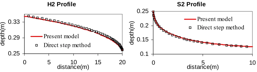
In the first case, formation of a sub-critical H2 and a super-critical S2 profile along a channel was simulated by the model. Flow discharge of 1.2

s

m

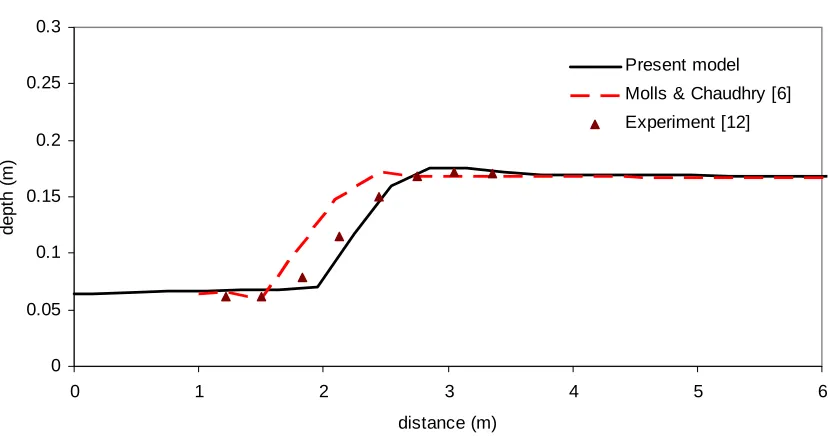
3 _{was assumed in a channel 3m wide with a}

manning roughness coefficient equal to 0.015. Bed slope of the steep channel was 0.05. Water surface profiles, calculated by the model for these profiles, conform well to the direct step method [25] as shown in Figure 2. It should be noted that in both of these profiles water surface gradient is very sharp where the flow approaches the critical depth. In the next test case, water surface profile was calculated along a steep slope following a mild one. Theoretically, critical depth occurs at the junction of the two slopes with water surface gradient approach infinity at this point. Though an infinite water surface slope was not calculated at the junction of the two slopes, water surface elevation predicted by the model is very close to that calculated from the direct step method (Figure 3). The critical depth is 0.294m in this problem in comparison with 0.284m calculated from the numerical model. The error of the model is 3.4% at the point with sharpest water surface gradient. Formation of a hydraulic jump was simulated by the model in the next test case. Molls and Chaudhry [6] compared the results of their numerical model for calculation of a hydraulic jump with experimental data of Gharangik and Chaudhry [12]. The experimental channel was 0.46m wide and with zero slope. Flow velocity and

S2 Profile

0.1 0.15 0.2 0.25

0 5 10

distance(m)

de

pt

h

(m

) Present model

Direct step method

H2 Profile

0.25 0.29 0.33

0 5 10 15 20

distance(m)

de

pt

h

(m

)

Present model Direct step method

depth upstream of the jump was 0.064m and 1.826 m/s respectively (Fr = 2.3). To get convergence, artificial viscosity was introduced in the Molls and Chaudhry’s model. The present model was applied in this case and the results are shown in Figure 4.

The results of Molls and Chaudhry [6] are also given in this Figure. Results show that the present model can predict the location of the jump accurately, without using any artificial viscosity. It should be noted that to find the minimum

0.15 0.2 0.25 0.3 0.35 0.4 0.45 0.5

0 5 10 15 20 25 30

distance(m)

d

ept

h(m

)

Present model

Direct step method

M2 Profile

S2 Profile

Figure 3. Mixed sub- and super-critical flow along a channel with two slopes.

0 0.05 0.1 0.15 0.2 0.25 0.3

0 1 2 3 4 5 6

distance (m)

dept

h (

m

)

Present model

Molls & Chaudhry [6]

Experiment [12]

acceptable value for artificial viscosity trial and error is necessary [6].

In the next test case, combination of different profiles and a hydraulic jump in channels with

two different slopes was considered. The first channel was steep, 8.75m long, and the second channel was mild and 38.75m long. At the beginning of the steep channel (inlet section) the

0 0.1 0.2 0.3 0.4 0.5 0.6 0.7

0 5 10 15 20 25 30 35 40 45

distance (m)

el

ev

at

io

n (m

)

Present model Bed Level

Direct step method

S2

M3

Jump

M2

Figure 5. Water surface profile along two channels with steep and mild slopes.

0 0.2 0.4 0.6 0.8 1

-1 -0.8 -0.6 -0.4 -0.2 0

y/(B/2)

U/

U

m

equation 38 wall function

younus&Chaudhry[15] Rodi [27]

exp. x/h=60 exp. x/h=150 exp. x/h=100 exp. x/h=100

y B CL

flow depth is 0.15 m. Super critical flow in the steep channel forms a S2 profile. In the mild slope first a M3 profile is formed which is followed by a hydraulic jump. Since a low tail water depth (0.2 m) is assumed at outlet, a M2 profile is formed immediately after the jump and this profile ends with the tail water depth at the channel outlet. This case was considered as a complex flow condition with combination of super- and sub-critical flows and a hydraulic jump. Calculation of water surface profile with direct step method in this case needs some effort to find the location of the hydraulic jump, and each profile needs to be calculated separately and then combined manually. However, the present model can calculate the water surface position along the whole length of the channels with the known boundary conditions only at the inlet and the outlet. The results are shown in Figure 5 and they indicate the accuracy of the model in this calculation.

In the above examples the side walls shear stresses were ignored. In the direct step method on the other hand the hydraulic radius was assumed to be equal to the flow depth which this also means no friction effect from the side walls. This assumption is acceptable if width to depth ratio is large. However wall shear stress has considerable effects on water surface profile if the channel is narrow. Molls et al. [25] used the hydraulic radius

of the channel cross section and distributed it among all cells across the channel. In this way, water surface profile calculated by the numerical model conforms with the direct step method in which hydraulic radius is used instead of flow depth. However in this method a uniform velocity profile will be calculated across the channel and the advantage of the 2-D model will be lost. If it is assumed that shear stress at side walls can be calculated in the same way as at the channel bed, wall friction can be included in the numerical model by replacing (14) with the following equation only for cells adjacent to walls.

y

x

y

h

h

v

u

n

g

S

_p

⎟⎟

∆

∆

⎠

⎞

⎜⎜

⎝

⎛

∆

+

+

−

=

1

3 1

2 2 2

(36)

Alternatively the well known wall function [26] can be employed to take into account the wall shear stress. To implement this method the following term should be added to the source term of u-momentum for the wall along x direction.

x

h

u

u

S

wall _{p wall wall}

u

=

−

∆

2 *

)

sgn(

(37)

in which _up is the velocity at nearest node to the wall and

u

_*wall is wall shear velocity that is

0 500 1000 1500 2000 2500 3000 3500 4000 4500 5000

0.5 0.55 0.6 0.65 0.7 0.75 0.8 0.85 0.9 0.95 1

N

o

. o

f Ite

ra

ti

o

n

1 . 0

=

p

α

2 . 0

=

p

α

3 . 0

=

p

α

4 . 0

=

p

α

5 . 0

=

p

α

55 . 0

=

p

α

v u,

α

calculated from wall function. For rough boundary this reads [26]:

⎟⎟

⎠

⎞

⎜⎜

⎝

⎛

∆

=

s wall

p

k

y

u

u

2

30

ln

1

*

κ

(38)

in the above equation

k

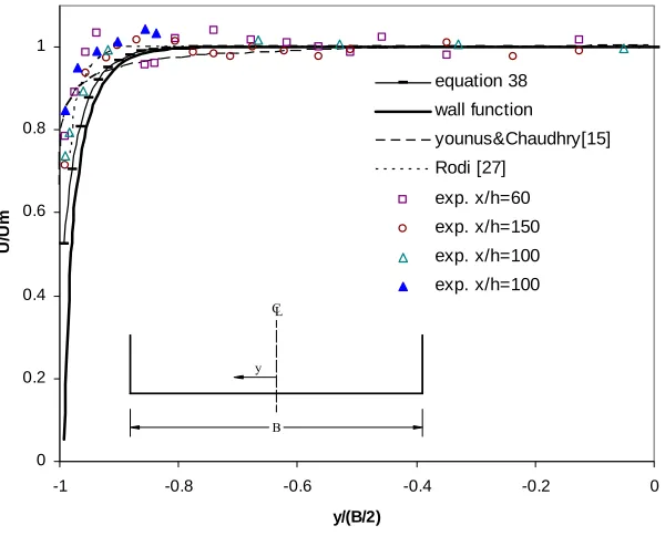
_s is the effective height of wall roughness.

To check the numerical model for calculation of velocity profile across the channel, it is compared with the results of experimental data presented by Rodi [27] and two other numerical models presented by Rodi [27] and Younus and Chaudhry [15]. A depth averaged k-ε turbulence model is utilized in these two studies. The experimental data is for a channel with width to depth ratio equals to 30 and n = 0.029. Here, a rectangular channel is assumed with a normal depth of 1 m and width of 30 m. The slope of this channel is considered equal to 0.001.

The results of the model are compared with experimental data [27] and numerical models of Rodi [27] and Younus and Chaudhry [15] in Figure 6. This Figure shows a generally satisfactory agreement between the predicted velocity profile

and experimental data. The present model also agrees well with both numerical models of Rodi [27] and Younus and Chaudhry [15]. It should be noticed that both of these models use a two equation k-ε turbulence model whereas in the present study a zero equation model is used. Model of Rodi conforms better with experimental results since the channel specifications (that is width, depth and slope) as was in the experiments were used by him. In contrast only width to depth ratio and Manning’s roughness coefficient were available in the present study and therefore channel specifications were assumed so that to conform with these values. It also can be seen that both methods used for calculation of wall friction give similar results.

5. THE ROLE OF UNDER-RELAXATION FACTORS

Under-relaxation factors are necessary in the model to prevent divergence. Barron and Salehi [28] studied the range of under-relaxation factors which guarantees convergence for solution of 2D Navier-Stokes equations. Based on their experience

0 2000 4000 6000 8000 10000 12000 14000 16000 18000

0 0.1 0.2 0.3 0.4 0.5 0.6 0.7

N

o

. of I

ter

at

ion

H2 S2

p

α

0 2000 4000 6000 8000 10000 12000 14000 16000 18000

0 0.1 0.2 0.3 0.4 0.5 0.6 0.7

N

o

. of I

ter

at

ion

H2 S2

0 2000 4000 6000 8000 10000 12000 14000 16000 18000

0 0.1 0.2 0.3 0.4 0.5 0.6 0.7

N

o

. of I

ter

at

ion

H2 S2

p

α

2 . 0 1

.

0 ≤α_p ≤ was safe, but a value of 0.2 was recommended for minimum

number of

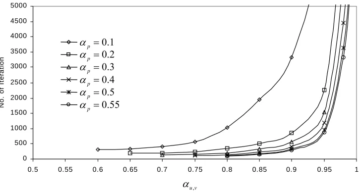
iteration. For momentum equation they found a safe range between 0.1 and 0.9 and value 0.8-0.9 was recommended for fastest convergence. In the present study it was noticed that the safe range of under-relaxation factors is different for sub- and super-critical flows. It was also found that the safe range of

α

_u,vdepends on

α

_pand vice versa. In the case of sub-critical H2 profile, a wide range of under-relaxation factors yielded converged solution. Minimum number of iteration was achieved with

α

_p

=

0

.

55

and

α

_u

=

0

.

8

. Safe range of

α

_ufor the sub-critical H2 profile is given in Figure 7 for various values of

α

_p. It can be seen that as

α

_p decreases, a wider range of

α

_u gives a converged solution. However with reducing

α

_p, number of iteration increases too. On the other hand with a constant

α

_p, number of iteration decreases as

α

_u decreases. Wider range of

α

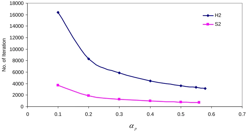
_pwas obtained for converged solution in the present study compared with Barron and Salehi [28].

In the case of super-critical flow, i.e. S2 profile, converged solution was achieved when

α

_uwas close to unity. With this

α

_u, a wide range of

α

_p from close to 0.1 to about 0.6 could be used. Figure 8 compares number of iteration in sub-critical H2 and super-sub-critical S2 profiles for different

α

_p and

α

_u

=

0

.

98

.

With mixed sub- and super-critical flows similar to a super-critical flow

α

_u close to unity is necessary for a converged solution. It should be noticed that the initial values assumed for the variables affect the safe range of under-relaxation factors.

6. CONCLUSION

The present paper deals with simulation of mixed sub- and super-critical flows in open channels with

an implicit numerical scheme. Unlike many previous models, there is no need for artificial viscosity in the present model. The well known two dimensional shallow water equations were applied and descretized on collocated grid in which all the variables are stored at cell centers. For the steady state equations a SIMPLEC like algorithm was developed for depth-velocity coupling Convection and diffusion terms were discretized using Power law scheme. Under relaxation factor for momentum and depth correction equations were necessary to get convergence in the iterative solution as is common in the implicit schemes. To avoid checker board depth fluctuation, the momentum interpolation proposed by Rhie and Chow [20] was used in calculating velocities on cell faces.

The model was verified with different test cases including various water surface profiles, hydraulic jump and combination of sub- and super-critical profiles with sharp water surface gradient. Wide range of under-relaxation factors yielded converged solution for sub-critical flows. However, minimum number of iteration was found with

α

u

=

0

.

8

and

α

p

=

0

.

55

. For super-critical

or combination of sub- and super-critical flows converged solution is achieved with

α

_u close to unity. With this

α

_u a wide range of

α

_p from 0.1 to about 0.6 can be used. It was also experienced that initial flow conditions affect the safe range of under-relaxation flows. In another test the numerical model was used to calculate velocity profile across a rectangular channel. Two different methods were used for including channel wall friction. The comparison of results with experimental data and two other numerical models showed good agreement.

7. REFERENCES

1. Kuipers, J. and Vreugdenhil, C. B., “Calculation of Two-Dimensional Horizontal Flow”, Rep. S163, Part 1, Delft Hydraulics Lab., Delft, Netherlands, (1973).

2. McGuirk, J. J. and Rodi, W. A., “Depth-Averaged Mathematical Model for the Near Field of Side Discharge into Open-Channel Flow”, J. Fluid Mech., Vol. 86(4), (1978), 761-781.

of Flow Pattern in Rivers”, J. Hydr. Div., ASCE, Vol. 108, (HY11), (1982), 1296-1310.

4. Chapman, R. S. and Kuo, C. Y., “Application of the Two-Equation k-ε Turbulence Model to a Two-Dimensional, Steady, Free Surface Flow Problem with Seperation”, Int. J. for Numer. Methods in Fluids, Vol. 5, (1985), 257-268.

5. Tingsanchali, T. and Maheswaran, S., “2-D Depth-Averaged Computation Near Groyne. J. Hydr. Engrg., ASCE ,Vol. 116(1), (1990), 71-86.

6. Molls, T. and Chaudhry, M. H., “Depth-Averaged Open-Channel Flow Model”, J. Hydr. Engrg., ASCE, Vol. 121(6), (1995), 453-465.

7. Ye J. and McCorquodale J. A., “Depth-Averaged Hydrodynamic Model in Curvilinear Collocated Grid”, J. Hydr. Engrg., ASCE, Vol. 123(5), (1997), 380-388. 8. Klonidis, A. J., Soulis, J. V., “An Implicit Scheme for

Steady Two-dimensional Free-Surface Flow Calculation”, J. Hydr. Res., IAHR, Vol. 39(4), (2001), 393-402.

9. Weerakoon, S. B., Tamai, N. and Kavahara, Y., “Depth-Averaged Flow Computation at a River Confluence”, Proc. Ins. Civil Engrg. Water & Maritime Engrg., Vol. 156(1), (2003), 73-83.

10. Fennema, R. and Chaudhry, M. H., “Explicit Methods for 2-D Transport Free-Surface Flows”, J. Hydr. Engrg., ASCE, Vol. 116(8), (1990), 1013-1034.

11. Bidone, G., “Observation, Sur le Hauteur du Ressaut Hydraulique en 1818”, Report (in French), Royal Academy of Sciences, Turin, Italy, (1819).

12. Gharangik, A. and Chaudhry, M. H., “Numerical Simulation of Hydraulic Jump”, J. Hydr. Engrg, ASCE, Vol. 117(9), (1989), 1195-1211.

13. Chaudhry, M. H., “Open Channel Flow”, PRENTICE-HALL, (1993).

14. Meselhe, E. A., Sotiropoulos, F. and Holly, F. M., “Numerical Simulation of Transcritical Flow in Open Channels”, J. Hydr. Engrg., ASCE, Vol. 123(9), (1997), 774-783.

15. Younus, M., Chaudhry, M. H., A Depth-Averaged k-e Turbulence Model for the Computation of Free-Surface Flow”, J. Hydr. Res., IAHR, Vol. 326(3), (1994),

414-436.

16. Zhou, J. G. and Stansby, P. K., “2D Shallow Water Flow Model for the Hydraulic Jump”, Int. J. for Numer. Methods in Fluids , Vol. 29, (1999), 375-387.

17. Zhou, J. G., “Velocity-Depth Coupling in Shallow-Water Flows”, J. Hydr. Engrg., ASCE, Vol. 121(10), (1995), 717-724.

18. Patankar, S. V., “Numerical Heat Transfer and Fluid Flow”, McGraw-Hill, (1980).

19. Lai, C. J. and Yen, C. W., “Turbulent Free Surface Flow Simulation using a Multilayer Model”, Int. J. Numer. Meth. Fluids, Vol. 16, (1993), 1007-1025.

20. Rhie, C. M. and Chow, W. L., “Numerical Study of the Turbulent Flow Past an Airfoil Trailing Edge Separation”, AIAA J., Vol. 21(11), (1983), 1525-1532.

21. Majumdar, S., “Role of Underrelaxation in Momentum Interpolation for Calculation of Flow with Nonstaggered Grids”, Numer. Heat Transfer, Vol. 13, (1988), 125-132.

22. Olsen, N. R. B., “CFD Algorithms for Hydraulic Engineering: Class Notes 2000”, Available on Internet at http://www.bygg.ntnu.no/~nilsol/cfd/cfdalgo.pdf. 23. Wang, Y., Komori, S., “Comparison of Using Cartesian

and Covariant Velocity Components on Non-orthogonal Collocated Grids”, Int. J. Numer. Meth. Fluids , Vol. 31, (1999), 1265-1280.

24. Chow, V. T., “Open-Channel Hydraulics”, McGRAW-HILL, (1959).

25. Molls, T., Zhao, G. and Molls, F., “Friction Slope in Depth-Averaged Flow”, J. Hydr. Engrg., ASCE, Vol. 124(1), (1998), 81-85.

26. Launder, B. E. and Spalding, D. B., “The Numerical Calculation of Turbulent Flows”, Comput. Methods Appl. Mech. Eng., Vol. 3, (1974), 264-287.

27. Rodi, W., “Turbulence Models and Their Application in Hydraulics: A State of the Art Review”, Presented by IAHR Delft, The Netherland, (1980).