RESEARCH NOTE
OPTIMAL LOAD OF FLEXIBLE JOINT MOBILE
ROBOTS STABILITY APPROACH
M. H. Korayem and H. Ghariblu
Department of Mechanical Engineering, Iran University of Science and Technology Tehran, Iran, [email protected]
A. Basu
Department of Mechanical Engineering, University of Wollongong Wollongong, NSW, Australia, [email protected]
(Received: September 9, 2003 – Accepted in Revised Form: April 4, 2004)
Abstract Optimal load of mobile robots, carrying a load with predefined motion precision, is an important consideration regarding their applications. In this paper a general formulation for finding maximum load carrying capacity of flexible joint mobile manipulators is presented. Meanwhile, overturning stability of the system and precision of the motion on the given end-effector trajectory are taken into account. The main constraints applied for the presented algorithm are torque capacity of actuators, limited error bound for the end-effector and overturning stability during the motion on the given trajectory. In order to verify the effectiveness of the presented algorithm, a simulation study considering a compliant joint two-link planar manipulator mounted on a differentially driven mobile base is explained in details.
Key Words Optimal Load, Overturning Stability, Base Mobility, Joint Elasticity
ﻩﺪﻴﻜﭼ
ﻩﺪﻴﻜﭼ
ﻩﺪﻴﻜﭼ
ﻩﺪﻴﻜﭼ
ﻞﺒﻗ ﺯﺍﺮﻴﺴﻣﻚﻳ ﺭﺩﺍﺭﺭﺎﺑﺪﻳﺎﺑﻪﻛ ﺖﺳﺍﻱﺩﺭﺍﻮﻣ ﺭﺍﺪﺧﺮﭼ ﻲﺗﺎﺑﺭ ﻱﺎﻫﻭﺯﺎﺑﻢﻬﻣ ﻱﺎﻫﺩﺮﺑﺭﺎﻛﺯﺍ ﻲﻜﻳ
ﺪﻨﻨﻛ ﻞﻤﺣ ﻲﺼﺨﺸﻣ ﺖﻗﺩ ﺎﺑ ﻡﻮﻠﻌﻣ
. ﺭﺎﺑ ﻞﻤﺣ ﺖﻴﻓﺮﻇ ﺮﺜﻛﺍﺪﺣ ﻦﻴﻴﻌﺗ ﻲﺗﺎﺒﺳﺎﺤﻣ ﺵﻭﺭ ﻦﻳﺍ ﺭﺩ ،ﻦﻳﺍﺮﺑﺎﻨﺑ
ﺩﺩﺮﮔ ﻲﻣ ﻪﺋﺍﺭﺍﺺﺨﺸﻣ ﺮﻴﺴﻣ ﻚﻳ ﺭﺩ ﺭﺍﺩ ﺥﺮﭼ ﻲﺗﺎﺑﺭ ﻱﺎﻫﻭﺯﺎﺑ
. ﻞﺻﺎﻔﻣ ﻦﺘﻓﺮﮔﺮﻈﻧ ﺭﺩ ﺎﺑ
ﺭﻮﻃ ﻪﺑ ﻚﻴﺘﺳﻻﺍ
ﺭﻮﻈﻨﻣ ﻪﻠﺌﺴﻣ ﻞﺣ ﺭﺩ ﺰﻴﻧ ﺭﺎﺑ ﺖﻛﺮﺣ ﺖﻗﺩ ﺪﻴﻗ ﻭ ﻲﻧﻮﮔﮊﺍﻭ ﻞﺑﺎﻘﻣ ﺭﺩ ﻢﺘﺴﻴﺳ ﻲﺘﻛﺮﺣ ﻱﺭﺍﺪﻳﺎﭘ ﺪﻴﻗ ﻥﺎﻣﺰﻤﻫ ﻲﻣ ﺪﻧﻮﺷ
.
ﺎﻫﺕﺎﺑﺭﺎﺠﻨﻳﺍﺭﺩﻪﻛﺖﺳﺍﻦﻳﺍﻞﺒﻗﻞﺼﻓﺎﺑﻞﺼﻓﻦﻳﺍ ﺰﻳﺎﻤﺗﻪﺟﻭﻦﻳﺍﺮﺑﺎﻨﺑ ﻱ
ﺭﺍﺪﺧﺮﭼﻪﻳﺎﭘﺎﺑﻙﺮﺤﺘﻣ
ﺪﻴﻗ ﻭﺎﻫﺭﻮﺗﻮﻣ ﺭﻭﺎﺘﺸﮔﺪﻴﻗ ﺮﺑﻩﻭﻼﻋ ﻭﻪﺘﻓﺮﮔﺭﺍﺮﻗ ﺮﻈﻧ ﺪﻣ
ﺪﻴﻗ ،ﺏﻮﻠﻄﻣﺮﻴﺴﻣﺭﺩ ﺭﺎﺑ ﺖﻛﺮﺣ ﺯﺎﺠﻣ ﻱﺎﻄﺧ
ﺩﻮﺷﻲﻣﻩﺩﻭﺰﻓﺍﺖﻛﺮﺣ ﻦﻤﺿﻲﻧﻮﮔﮊﺍﻭﺯﺍﻱﺮﻴﮔﻮﻠﺟﺮﺑﻲﻨﺒﻣﻱﺮﮕﻳﺩ
. ﻥﺎﻜﻣﻪﻛﻞﺒﻗﻞﺼﻓﻑﻼﺧﺮﺑﻦﻴﻨﭽﻤﻫ
ﻡﺎﺠﻧﺍ ﻪﻳﺎﭘ ﻭﻭﺯﺎﺑ ﻥﺎﻣﺰﻤﻫ ﺖﻛﺮﺣ ﺎﺑ ،ﺮﻈﻧﺩﺭﻮﻣ ﺮﻴﺴﻣ ﺭﺩ ﺭﺎﺑ ﻞﻤﺣ ،ﺩﻮﺑ ﻩﺪﺷ ﺖﻴﺒﺜﺗ ﺭﺎﺑ ﺖﻛﺮﺣ ﻦﻤﺿ ﻪﻳﺎﭘ ﻲﻣ ﺩﺮﻳﺬﭘ
. ﻭﺵﻭﺭﺩﺮﺑﺯﺎﻛﻥﺩﺍﺩﻥﺎﺸﻧﻱﺍﺮﺑ
ﻭﺩﻱﻭﺯﺎﺑﻚﻳ،ﻞﻣﺎﺷﻱﺯﺎﺳﻪﻴﺒﺷﻝﺎﺜﻣ ﻪﻧﻮﻤﻧﻭﺩﻢﺘﻳﺭﻮﮕﻟﺍ ﺖﺤﺻ
ﺖﺳﺍﻪﺘﻓﺮﮔﺭﺍﺮﻗﻩﺩﺎﻔﺘﺳﺍﺩﺭﻮﻣ،ﻩﺪﺷﺐﺼﻧﺭﺍﺩﺥﺮﭼﻙﺮﺤﺘﻣﻪﻳﺎﭘﻚﻳﻱﻭﺭﺮﺑﻪﻛﻱﺍﻪﺤﻔﺻﻲﻜﻨﻴﻟ
.
ﺖﻟﺎﺣﺭﺩ
ﻲﻣﻥﺁﻞﺣﺵﻭﺭﻭﺩﺍﺯﺎﻣﺩﺍﺯﺁ ﺕﺎﺟﺭﺩﺚﺤﺑﺮﺑﺪﻴﻛﺎﺗﻭﻩﺪﺷﺽﺮﻓﺐﻠﺻﺕﺎﺑﺭﺭﺎﺘﺧﺎﺳﻝﻭﺍ ﺪﺷﺎﺑ
. ﻪﻠﺣﺮﻣﺭﺩ
ﻦﺘﻓﺮﮔﺮﻈﻧ ﺭﺩﺎﺑﺪﻌﺑ
ﻪﺑ ﻱﺍﺮﺑﺖﻛﺮﺣ ﻱﺭﺍﺪﻳﺎﭘ ﻭﺖﻗﺩﻱﺎﻫﺪﻴﻗﻝﺎﻤﻋﺍ ﺮﺑﺪﻴﻛﺎﺗ،ﺕﺎﺑﺭﻱﺍﺮﺑ ﻚﻴﺘﺳﻻﺍﻞﺻﺎﻔﻣ
ﻲﻣﺭﺎﺑﻞﻤﺣﺖﻴﻓﺮﻇﻥﺩﺭﻭﺁﺖﺳﺩ ﺪﺷﺎﺑ
.
1. INTRODUCTION
The literature on determining DLCC on different types of robotic systems is fairly rich. Thomas, et al. [1] used the load carrying capacity as a criterion for sizing the actuator at the design stage of robotic manipulators. Wang and Ravani [2] developed a
kinematically redundant manipulators. Korayem and Ghariblu [6] developed an algorithm for finding the DLCC on rigid mobile manipulators. In their work the stability and flexibility are not taken into account. Also, some researchers have studied the stability of mobile manipulators. Some of the earlier work discussed only the static stability [7-8] and some others were concerned with the dynamic stability [9-10]. Moreover, there is some research work on carrying heavy loads or application of large forces by mobile manipulators [11]. But, none of these works has considered the DLCC finding on mobile manipulators.
In this paper, the dynamic load carrying capacity of flexible joint mobile manipulator is investigated. The main focus of this research work is small vehicles with considerations of overturning stability and elasticity on joints. At the first stage, the dynamics of these types of systems is introduced in their general form. Then, for a general case, the algorithm of finding dynamic load carrying capacity for mobile manipulators on a given trajectory is presented. Finally, simulation studies are conducted for a two-link mobile planar mobile manipulator with elastic joints.
2. DYNAMIC MODEL OF FLEXIBLE JOINT MOBILE MANIPULATOR
If the degrees of freedom of base and manipulator
are denoted by
n
b andn
m respectively, and endeffector degrees of freedom is denoted by
m
,then in the overall system there will be a
kinematic redundancy of the order of
r
=
n
−
m
,where
n
=
n
b+
n
m. There are different types ofconstraints that can be applied to a robotic system in order to solve the redundancy resolution [10, 12]. One of these methods that are well
known [12] uses
r
as an additional user definedby kinematic constraint equations with the general
form of
x
=
g
(
q
)
, as a function of motionvariables
q
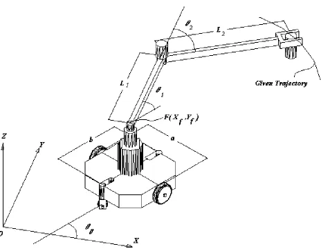
. This method results in a simple andon line coordination on control of a mobile manipulator during the motion. This paper will follow this method because of its convenient implementation. Referring to Figure 1, the
configuration vector of the mobile base is shown
by T
r fr fr
br
x
y
q
r
=
(
,
,
θ
0)
, wherex
fr,
y
fr are theposition coordinate at point F where manipulator is
attached to the mobile base and
θ
0r is theorientation angle. Subscript r is pointed on
assuming rigid case on the desired trajectory. Meanwhile, the configuration vector of the manipulator in rigid case is shown by
T mr r
r mr
q
r
=
(
θ
1,
θ
2,
....,
θ
)
, with generally m links. The overall configuration of the mobile manipulator assuming rigid structure is shown by)
,
(
1
q
brq
mrq
r
=
r
r
. Simultaneously, the overallconfiguration of the mobile manipulator assuming flexibility on joints is shown by
)
,
(
2
q
bfq
mfq
r
=
r
r
.The dynamic equations of motion are obtained using a Lagrangian approach as follows:
, 0 ) ( ) ( ) , ( )
(q1 q1+C q1 q1 q1+G q1 +K q1−q2 =
D r r&& r r& r& r r r
(1)
τr
r r r
&&2+K(q2 −q1)= q
Ir (2)
where D(qr1) is the inertia matrix for the
associated rigid system, C(q1,q1)
r &
r is the vector of
damping, Coriolis and centrifugal forces, G(qr1) is
the vector of forces due to gravity, ]
....,
[k1, k2, kn
diag
K= is a diagonal matrix
of restoring force constant modeling the joint
elasticity, Ir is motor inertia, and τr is the
generalized force inserted to the actuator.
3. FORMULATION OF DLCC FOR A PREDEFINED TRAJECTORY
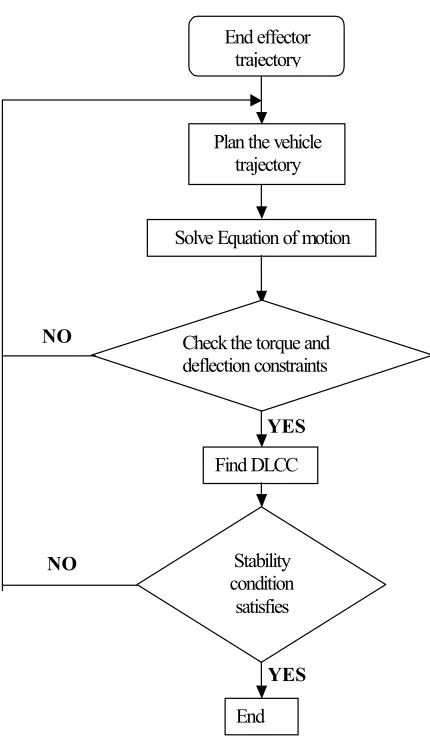
flexibility. This consideration can be taken into account in DLCC determination by imposing a constraint on the end-effector deflection, in addition to the actuator torque constraint imposed alone for rigid manipulators. Otherwise, deflection of the end-effector can cause excessive deflection from the predefined trajectory, even though the joint torque constraints are not violated. By considering the actuator torque and deflection constraints and adopting a logical computing method, the maximum load carrying capacity of a mobile manipulator for predefined trajectory can be computed. Meanwhile, it is possible for the known trajectory and computed maximum load that stability conditions not be satisfied during the motion. Using the method of Zero Moment Point (ZMP) method, dynamic stability of the system for
the known trajectory and DLCC can be checked. If stability conditions are not fulfilled, then another trajectory for the vehicle for the same end-effector trajectory should be selected, until the stability conditions are satisfied. Therefore, the algorithm shown in Figure 2 is proposed for finding the DLCC of the system.
3.1. Formulation of the Actuator Torque
Constraint
The actuator torque constraint is formulated on the basis of typical torque-speed characteristics of DC motors.• •
− − =
− =
q k k T
q k k T
lb ub
2 1
2
1 (3)
Here, k1 =Ts and k2 =Ts/ωnl, Ts is the stall
torque and ωnl is the maximum no-load speed of
the motor. Tub and Tlb are the upper and lower
bounds of the allowable torque. Other actuation systems can also be dealt with similarly. Using Equations 3 the upper and lower bounds of motor torques are found and then the available torque for carrying load can be expressed as:
i l i lb i i l i ub
i (T ) (τ ) , τ (T ) (τ )
τ+ = − − = − (4)
Thus, the maximum allowable torque at i-th joint is
equal to:
{
+ −}
+ =
i i
i τ τ
τ max , (5)
It is necessary to introduce the concept of load coefficient complying with the torque actuator
constraint that can be calculated for each point j, j
= 1, 2, ..., p of a given trajectory as follows
} p ...., , , i , } max{ } max{ } { min{ ) C ( nl l i max j
a =12
τ − τ τ = (6)
where τnl is the no-load torque and:
} ) ( ..., , ) ( , ) ( max{ }
max{τl = τl 1 τl 2 τl p
(7) } ) ( ..., , ) ( , ) ( max{ }
max{τnl = τnl 1 τnl 2 τnl p
3.2. Formulation of the Accuracy Constraint
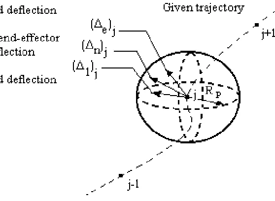
A constraint should be imposed in such a way that the worst case, which corresponds with the least DLCC, be used to determine the maximum load. For a given discretized trajectory, the no load
deflection (∆n)j and deflection with added end
effector mass (∆e)j, are calculated for j=1, 2, ...,
p (Figure 3). Using the computational procedure,
the additional mass at the end effector changes both direction and magnitude of the deflection. But, as long as the magnitude of the deflection is less than or equal to an allowable value, the robot is considered to remain capable of executing the given trajectory. In other words, only the
magnitude of the deflections (∆n)j and (∆e)j
need to be considered in this context. This prompted the use of a ball type boundary of
radius Rp centered at the desired position on the
given trajectory. Although, (∆l)j as load
deflection and (∆n)j and (∆e)j are generally
vectors of different directions, the magnitude increase due to the added mass at the end effector is linearly related to mass [5]. The difference between the allowable deflection and the
End effector trajectory
Solve Equation of motion
Stability condition
satisfies
End Plan the vehicle
trajectory
Check the torque and deflection constraints
Find DLCC
Figure 2. Algorithm of finding DLCC.
YES NO
NO
magnitude of the deflection with added end
effector mass at point j, Rp −(∆e)j can be
regarded as the remaining amount of end effector deflection which can still be accommodated at
point j of the given trajectory. This remaining
amount of end effector deflection indicates how
many loads can be carried through point j without
violating the deflection constraint. Therefore, it is necessary to introduce the concept of a load
coefficient(Cp)j for point j, j=1, 2,..., p as
follows: } max{ } max{ ) ( ) ( n e j e p j p R C ∆ − ∆ ∆ −
=
(8)
3.3. Formulation of the Stability Constraint
To analyze the stability of a mobile manipulator on its motion, the ZMP criterion is used, which is discussed and developed by other researchers [9-10]. In their model, the inertia effect of rigid body that is an important consideration i n t h e s y s t e m d y n a m i c s i s u s e d i n t h i s paper.
The ZMP is defined as a point on a vehicle’s moving floor where the sum of all external, gravity and inertial forces on the system are
equal to zero. If the i-th rigid part of the system
has a mass mi, inertia tensor Ii with respect to
its center of mass with coordinate T
i i i y z
x , , )
( , then ZMP coordinate can be
computed as follows [10].
∑
∑
∑
∑
+ − − + =i i i i
i i i i i i i i i i x zmp x ) g z ( m ) M ( z x m x ) g z ( m x && && && (9)
∑
∑
∑
∑
+ − − + =i i i i
i i i i i i i i i i y zmp x ) g z ( m ) M ( z y m y ) g z ( m y && && &&
where Mi =Iiω&i +ωi×Iiωi and ωi is the angular
velocity of rigid body in the inertial reference frame. Using the recursive Newton-Euler formulation, ZMP coordinates can be easily computed with the following formulation:
y , y , zmp
)
F
(
)
T
(
x
1 0 1 0−
=
(10)
z , x , zmp)
F
(
)
T
(
y
1 0 1 0=
where T0,1 and F0,1 are the overall torque and force
applied to the vehicle in the inertial reference frame.
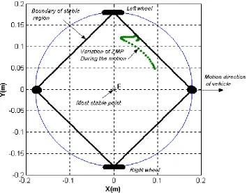
The stability index is defined as a measure for determining the value of stability from marginal condition as below:
region
stable
from
int
po
stable
most
of
ce
tan
dis
region
stable
of
boundary
from
ZMP
of
ce
tan
dis
S
=
The value of S = 1 corresponds to a condition
which ZMP is over or outside of the boundary of
stable region and S = 0 corresponds to a condition
which ZMP coincides with the most stable point (Figure 9).
3.4. Determining Maximum Load Carrying
Capacity
The load coefficient (C) is obtained as follows:}
....,
,
2
,
1
,
)
(
,
)
min{(
C
C
j
p
C
=
p j a j=
(11)
for the p number of discretized points of a
given trajectory. Then, the maximum mass that could be carried on the given trajectory is:
init load C m
m = ×
(12)
where m
initis the initial mass of the load.
4. SIMULATION RESULTS AND DISCUSSIONS
As shown in the Figure 1, the mobile manipulator consists of a two-link planar manipulator attached
at point F(xf, yf)on the middle of a
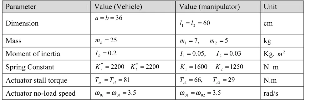
differentially driven vehicle with considering joint flexibility on sub system, vehicle and manipulator. The kinematic, dynamic and other necessary parameters are summarized in Table 1.
As shown in Figure 4, the path of the load i s a t wo -s e gme n t e d l i n e t h a t s t a r t s f r o m
the c oo rd ina te (x1 =1.0 m, y1=1.4 m) t o
intermediate point with coordinate ( x2 = 1.8 m,
y2 = 2.0 ) and ends at point with coordinate
) 8 . 1 , 8 . 2
(x3 = m y3= m .
The velocity of the end effector at each segment is as follows:
2
,
1
4
3
4
3
4
0
max=
≤
≤
−
=
≤
≤
=
≤
≤
=
i
t
t
t
at
t
t
t
t
t
t
at
i i i i iν
ν
ν
ν
where ti is the time of motion at each segment
TABLE 1. Parameters of the Simulation.
Parameter
Value (Vehicle)
Value (manipulator)
Unit
Dimension
a=b=36 l1=l2 =60cm
Mass
mb =25 m1=7, m2 =5kg
Moment of inertia
Ib =0.2 I1=0.05, I2 =0.03Kg.
m2Spring Constant
*=2200r
K
*=2200 l
K K1=1600
K2=1250
N. m
Actuator stall torque
Tsr =Tsl =81 Ts1=66, Ts2 =29N.m
Figure 4. The path of the mobile manipulator considering the load and vehicle motion.
Figure 6. Variation of ZMP point considering final path for the vehicle.
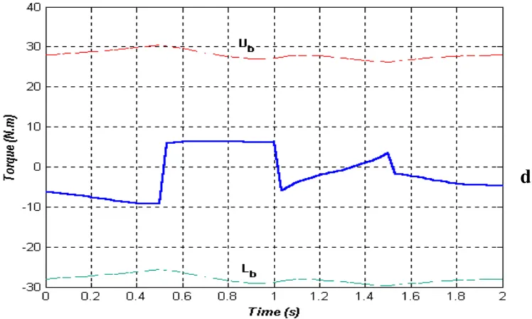
Figure 8. Joint torques for the final trajectory: (a) Vehicle right wheel, (b) Vehicle left wheel and (c)Manipulator first joint.
a
b
and the overall motion time is t1 + t2 = Tf = 2 sec.
To find suitable base trajectory, initially a linear path is selected for the vehicle, which starts from a
point with coordinate (x1 = 1.1 m, y1 = 0.5 m)
to the end point with coordinate (x1 = 2.8 m,
y1 = 1.6 m). The path of the load considering
joint flexibility is shown in Figure 4 for comparison with the desired path. In the Figure 5 it is seen that for the given end effector trajectory and initial selected path for the base and initial load that equals
kg
minit =1.0 , the ZMP lies outside the
polygonal stable region produced by lines which connects the base wheels together. Therefore, another path must be selected for the vehicle. A final path is selected for the vehicle, which starts from a point with coordinate
) m . y , m . x
( 1=10 1=10 to the end point with
coordinate (x1=2.8 m, y1=1.6 m). Figure 6
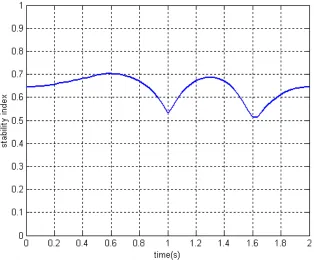
shows the variation of ZMP point during the motion considering final path for the vehicle. Also, Figure 7 shows the variation of stability index for both cases; initial and final vehicle paths. The corresponding exerted torques to vehicle and manipulator actuators, considering
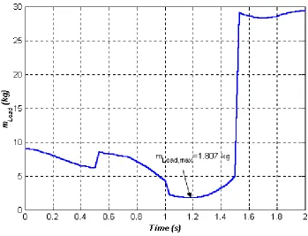
the final path for the vehicle, are shown in Figure 8. For the final motion, the equivalent dynamic load carrying capacity at each instant of time is shown in Figure 9. It can be seen that maximum load carrying capacity is equal to 1.807 kg.
Therefore, using kinematic redundancy of the systems, there are various ways of carrying a load from a desired trajectory. However it is possible that one of the constraints related to the torque, precision or stability be violated in one way or another. As shown in the simulation study, for the initial path selected for vehicle, the stability constraint is violated, which for the final vehicle path, the stability criterion is satisfied. Furthermore, none of the joint motors move with their full capacity.
5. CONCLUSION
A computational algorithm for finding dynamic load carrying capacity of flexible joint mobile manipulators is introduced. The actuator torque, motion accuracy and over-turning stability are
Figure 8. Joint torques for the final trajectory: (Continued from previous page) (d) Manipulator second joint.
considered as main constraints in the problem formulation. Due to combined motion of the vehicle and manipulator, the overall system has kinematic redundancy on its motion. Thus changing the vehicle motion for a predefined end effector trajectory is used to prevent system from overturning. In a simulation study, a two arm planar manipulator mounted on a differentially driven vehicle is considered for carrying a load on a given trajectory. It is seen that by changing vehicle motion for a predefined end effector trajectory, stability condition of mobile manipulator is assured and motion accuracy constraint is dominated in comparison to motor torque constraints and computed maximum load carrying capacity is found to be equal to 1.807 kg.
6. REFERENCES
1. Thomas, M. H., Yuan-Chou, C. and Tesar, D., “Optimal
Actuator Sizing for Robotic Manipulators Based on
Local Dynamic Criteria”, J. of Mechanisms,
Transmissions and Automation in Design, Vol. 107, (1985), 163-169.
2. Wang, L. T. and Ravani, B., “Dynamic Load Carrying Capacity of Mechanical Manipulators- Part 1: Problem Formulation”, J. of Dyn. Sys. Meas. and Control, Vol. 110, (1988), 46-52.
3. Korayem, M. H. and Basu, A., “Formulation and Numerical Solution of Elastic Robot Dynamic Motion with Maximum Load Carrying Capacity”, Robotica, Vol. 12, (1994), 253-261.
5. Korayem, M. H., and Basu, A., “Dynamic Load Carrying Capacity for Robotic Manipulators with Joint Elasticity Imposing Accuracy Constraints”, Robotic and Autonomous Systems, Vol. 13, (1994), 219-229.
6. Yue, S., Tso, S. K. and Xu, W. L., “Maximum Dynamic Payload Trajectory for Flexible Robot Manipulators with Kinematic Redundancy”, Mechanism and Machine Theory, Vol. 36, (2001), 785-800.
7. Korayem, M. H. and Ghariblu, H., “Maximum Allowable Load on Wheeled Mobile Manipulators Imposing Redundancy Constraints”, Robotics and Autonomous Systems, Vol. 44, No. 2, (2003), 151-159. 8. Fukuda, T., Fujisawa, Y., Kosuge, K., Arai, F., Muro, E.,
Hoshino, H., Miyazaki, T., Otobo, K. and Uehara, K., “Manipulator/Vehicle System for Man-Robot Cooperation”, Proc. of IEEE Int. Conf. on Rob. and
Autom., (1992), 74-79.
9. Papadopoulos, E. G. and Ray, D. R., “A New Measure of Tip over Stability Margin for Mobile Manipulators”,
Proc. of IEEE Int. Conf. on Rob. and Autom., (1996), 3111-3116.
10. Huang, Q., Sugano, S. and Tanie, K., “Coordinated Motion Planning for a Mobile Manipulator Considering Stability and Manipulation”, Int. J. of Robotic Research, (2000), 732-742.
11. Kim, J., et al., “Real Time ZMP Compensation Method
using Null Motion for Mobile Manipulator”, Proc. of IEEE Int. Conf. on Rob. and Autom., (2002), 1967-1972.
12. Rey, D. A., and Papadopoulos, E. G., “Online Automatic Tip-Over Presentation for Mobile and Redundant Manipulators”, Proc. of IEEE Int. Conf. on Intelligent Robots and Systems (IROS’97), (1997), 1273-1278. 13. Seraji, H., “A Unified Approach to Motion Control of