Please cite this article as: H. Mokhtari, A. Salmasnia, Fitting the Three-parameter Weibull Distribution by using Greedy Randomized Adaptive Search Procedure, International Journal of Engineering (IJE), TRANSACTIONS C: Aspects Vol. 30, No. 3, (March 2017) 425-432
International Journal of Engineering
J o u r n a l H o m e p a g e : w w w . i j e . i r
Fitting the Three-parameter Weibull Distribution by using Greedy Randomized
Adaptive Search Procedure
H. Mokhtaria, A. Salmasnia*b
a Department of Industrial Engineering, Faculty of Engineering, University of Kashan, Kashan, Iran
b Department of Industrial Engineering, Faculty of Engineering and Technology, University of Qom, Qom, Iran
P A P E R I N F O
Paper history:
Received 29 August 2016
Received in revised form 01 January 2017 Accepted 09 February 2017
Keywords: Statistical Inference Weibull Distribution
Greedy Randomized Adaptive Search Procedures
Grid Search
A B S T R A C T
The Weibull distribution is widely employed in several areas of engineering because it is an extremely flexible distribution with different shapes. Moreover, it can include characteristics of several other distributions. However, successful usage of Weibull distribution depends on estimation accuracy for three parameters of scale, shape and location. This issue shifts the attentions to the requirement for effective methods of Weibull parameters estimation. It is a known fact that the estimation procedure is inherently a very complicated procedure when the three-parameter Weibull distribution is of interest. Hence, this study suggests a computational approach, greedy randomized adaptive search procedures, with several neighborhood local searches to enhance the quality of estimations. Computational experiments are also implemented to assess the quality of estimations as opposed to benchmark grid search algorithm.
doi: 10.5829/idosi.ije.2017.30.03c.12
1. INTRODUCTION1
The probabilistic Weibull model is an extremely flexible distribution because of its different curve shapes. This property has made it capable in fitting of a wide range of experimental data very well and consequently has given rise to widespread real applications. For example, it is the most widely employed distribution for failure analysis in various types of systems in which decreasing and increasing hazard rates are taken into account [1]. Moreover, the Weibull distribution has been used in radar systems to model the dispersion of the received signal level caused by clutters. Furthermore, the distribution is especially useful for doing statistical analysis of satellite reliability and simulation of significant wave height [2]. Other application areas include wind energy potential [3], biomedical sciences [4], air quality determination [5], food products drying technology [6], model for growth/decline in product sales [7], and optimum adhesive thickness in structural adhesives joints [8].
1*Corresponding Author’s Email: [email protected] (A. Salmasnia)
The probability density function of the three-parameter Weibull distribution is as below [9]:
𝑓𝑋(𝑥; 𝛼, 𝛽, 𝛿) = 𝛽
𝛼(
𝑥−𝛿
𝛼 )
𝛽−1
𝑒(𝑥−𝛿𝛼 ) 𝛽
; 𝛼, 𝛽 > 0, 𝑥 ≥ 𝛿 (1)
where, 𝛼, 𝛽 and 𝛿 are known as the scale, shape and location parameters, respectively. Because of its importance, many techniques have been suggested to estimate the three-parameter Weibull distribution parameters. However, the most existing estimation approaches relaxes one of its parameters to estimate the other two because of a known fact that the estimation procedure of the three-parameter Weibull distribution family is intrinsically complicated. In real world situations, successful application of Weibull distribution depends on having appropriate statistical estimates of the three parameters.
designed. Section 5 discussed the computational results, and section 6 concludes the paper.
2. RELATED WORKS
Regarding the three-parameter Weibull distribution, Qiao and Tsokos [10] presented a stepwise algorithm including eight steps for fitting a Weibull distribution. Nosal and Nosal [11] employed array processing language and Monte Carlo simulation to investigate the
performance of the gradient random search
minimization procedure for estimating three parameters of Weibull distribution to a given data set. Teimouri et al. [12] classified the estimation techniques into five major categories: the approach of moments; the approach of maximum likelihood estimation; the approach of logarithmic moments; the percentile approach; and the approach of L-moments. They provided a comprehensive comparison of these estimation methods. Bartolucci et al. [13], Bartkute and Sakalauskas [14], Jukic etal. [15], Jukic and Markovich [16], and Markovich and Jukic [17] suggested moments-based approaches for estimation the Weibull distribution parameters. The most common way for estimation the parameters of the density function from an observed data set is the maximum likelihood estimation (MLE) technique [18-21]. Luus and Jammer [22] demonstrated that MLE gives the most reliable parameter estimation compared to the errors-in-variables and least-squares approaches. Ismail [23] employed a Newton–Raphson algorithm to maximize the MLE for hybrid censored data. He also through a Monte Carlo simulation calculated the mean square errors and biases of the MLE in order to investigate their performances.
Since the estimation procedure of the three-parameter Weibull distribution is a quite difficult problem, some researchers suggested intelligent-based heuristic approaches to discover satisfying solutions. Abbasi et al. [24] applied simulated annealing as one of the most popular meta-heuristics to maximize the likelihood function formed to estimate three-parameter Weibull distribution. Later on, in order to improve the performance of their method, Abbasi et al. [25] developed a hybrid variable neighborhood search and simulated annealing method. Furthermore, Abbasi et al. [26] suggested a neural network-based method which estimates the three parameters by using mean, standard deviation, median, skewness and kurtosis of the data. Wang [27] suggested bare bones particle swarm optimization algorithm to estimate the two-parameter Weibull distribution through maximizing MLE. Moeni et al. [28] developed a modified cross entropy method, as one of the modern simulation-based optimization methods, in the context of MLE of a three-parameter Weibull distribution. Yang and Yue [29] proposed a kernel density estimation-based method utilizing the
genetic algorithm and neural network to estimate the three-parameter Weibull distribution. Orkcu et al. [30] employed differential evolution algorithm to maximize the MLE function. Recently, Orkcu et al. [31] showed that the performance of particle swarm optimization considerably depends greatly on its control parameters such as acceleration coefficients and inertia weight in the parameter estimation problem of Weibull distribution.
For more details, we refer the interested readers to the surveys by Luus and Jammer [22] and Cousineau [32] which reviewed estimation methods for three-parameter Weibull distribution.
3. PARAMTER ESTIMATION USING MLE
Estimation theory plays an important role in statistical analysis and engineering designs. In the last decade, several techniques such as maximum likelihood estimation, moments method [33, 34], graphical procedure, and weighted least square method [35, 36] have been introduced to estimate parameters. Among the existing approaches to estimate the parameters of a given probability distribution based on a data set, the MLE method is the most popular estimation technique because of its applicability in complex estimation problems. Furthermore, it is widely known that MLE provides asymptotically unbiased estimators with the minimum variance.
This study suggests employing the MLE method to estimate three-parameters of Weibull distribution due to the desirable statistical properties of estimators obtained by this technique. Let 𝑥1, 𝑥2, … , 𝑥𝑛 be a random sample of size 𝑛 drawn from probability density function of the three-parameter Weibull distribution 𝑓𝑋𝑖(𝑥𝑖; 𝛼, 𝛽, 𝛿).
Since 𝑥𝑖𝑠 are independent, their joint probability density function is the product of the individual probability density functions. Consequently, the likelihood function for Weibull distribution is equal to Equation (2).
𝐿(𝑥1, 𝑥2, … , 𝑥𝑛; 𝛼, 𝛽, 𝛿) =
∏ 𝛽
𝛼(
𝑥𝑖−𝛿
𝛼 )
𝛽−1
𝑒(𝑥𝑖−𝛿𝛼 ) 𝛽
; 𝛼, 𝛽 > 0, 𝑥 ≥ 𝛿
𝑛
𝑖=1
(2)
The aim is to determine a vector value for 𝛼, 𝛽, and 𝛿
that maximizes the likelihood function. In practice, the maximization of the natural logarithm of the likelihood function, called the log-likelihood, is extremely more convenient. Hence, to maximize 𝐿, equivalently log-likelihood function is utilized, which for the three-Weibull distribution is as Equation (3).
𝐿𝑛(𝐿(𝑥1, 𝑥2, … , 𝑥𝑛; 𝛼, 𝛽, 𝛿)) = 𝑛𝐿𝑛 (𝛽𝛼) +
∑ [− (𝑥𝑖−𝛿
𝛼 )
𝛽
+ (𝛽 − 1)𝐿𝑛 (𝑥𝑖−𝛿
𝛼 )]
𝑛
𝑖=1
(3)
following system of differential equations. However, it is very hard to evaluate the gradient terms in this problem because of the large number of parameters and multi-modal nature the log-likelihood function for the three-Weibull distribution. Hence, solving system of Equations (4-6) and also applying classical gradient-based methods cannot be interesting ways.
𝜕𝐿𝑛(𝐿(𝑥1,𝑥2,…,𝑥𝑛; 𝛼,𝛽,𝛿))
𝜕𝛼 = 0 (4)
𝜕𝐿𝑛(𝐿(𝑥1,𝑥2,…,𝑥𝑛; 𝛼,𝛽,𝛿))
𝜕𝛽 = 0 (5)
𝜕𝐿𝑛(𝐿(𝑥1,𝑥2,…,𝑥𝑛; 𝛼,𝛽,𝛿))
𝜕𝛿 = 0 (6)
To overcome these difficulties, this study develops a numerical search method based on greedy randomized adaptive search procedures to handle the parameter estimation of three-parameter Weibull distribution as an optimization problem with log-likelihood objective function.
4. GREEDY RANDOMIZED ADAPTIVE SEARCH PROCEDURE
The problem of optimization to select among a finite number of options appears in industry frequently. Considerable researches have been carried out over the last three decades to devise optimal seeking techniques so as to converge to optimal solution without requiring any explicit evaluation of each option. This work has been treated with an increasing rise to the context of combinatorial optimization, and gains invaluable capability to solve real world problems. However, some open problems remain regarding finding global
optimum, local optimum trapping, premature
convergence, etc. In addition, most real world problems existing in industry are computationally intractable, or very large scale which make the use of exact methods more costly. In such situations, the application of heuristic and metaheuristics are common strategies in finding appropriate near optimal solutions with less computation difficulty. The success of these techniques is highly related to their capability in preventing to trap at local area, and utilizing the structural property of problem. To this end, some common remedy strategies like restart mechanisms, randomization process, and preprocessing can be utilized. By exploiting these mechanisms, different heuristic and metaheuristic search methods have been established which improves our ability to achieve acceptable solutions for difficult real world problems.
Among various heuristic and metaheuristic approaches which are available to the operations research audiences, the GRASP is a relatively new one. It is an iterative randomized sampling search method which gives a solution of the problem at each iteration.
The best solution obtained during all GRASP iterations is introduced as the final result. There are two phases during GRASP iterations: (i) construction phase in which an initial solution is constructed via an adaptive randomized greedy heuristic; and (ii) local search phase in which a heuristic is applied to current solution in hope of achieving a better solution. In current paper, we devise the various components in GRASP and to fit the parameters of Weibull distributions described in previous section. A general pseudo-code of GRASP is shown by Figure 1. The problem input is taken in Line
1 of the pseudo-code. In lines 2– 6, the GRASP iterations are executed. The iterations are terminated when stopping criterion like maximum number of iterations is met. The construction phase take places in Line 3 and the local search phase occurres in line 4. If an improvement happens, the update process runs in line 5. In subsequent sections, we describe these two phases with more details.
4. 1. GRASP Construction Phase A feasible
solution is iteratively generated in GRASP construction phase step by step by adding one element at a time. During one specific iteration of this phase, a greedy function is considered to order all of elements in a candidate solution list and recognize the next element to be added. The greedy function evaluates the appropriateness of each element to be selected. Since the appropriateness of each element is changed at each iteration of this phase, this method should be adaptive. This leads to reflecting the changes created by the last element selected in previous stage. The GRASP utilizes a list of top candidates which is entitled as restricted candidate list (RCL). To construct the RCL used in this phase, the incremental cost associated with the incorporation of element into the current partial solution is assessed by greedy function. At any GRASP iteration, the restricted candidate list RCL is made up of elements with the best incremental costs. This list can be limited by the number of elements in the list υ.
To randomly select one of the best candidates in the RCL, the GRASP uses a probabilistic mechanism. The selected element should not be necessarily the best one in the list in order to allow the GRASP for obtaining different diverse solutions at each iteration.
Procedure GRASP
1. Input Instance;
2. for Stopping criterion not satisfied
3. Construct greedy randomized solution;
4. Local search;
5. Update solution;
6. end
7. Return best solution found end GRASP
Figure 2 gives the pseudo-code for the GRASP construction phase. Line 1 initializes the solution to be generated in construction phase. The solution is constructed within loop in line 2 to 7, and the RCL is constructed in line 3 of pseudo-code. In lines 4 and 5 a candidate S is randomly chosen from RCL, and is used to form the solution. In line 6 of code, the greedy function is called and the effect of the selected element
S on the appropriateness associated with every element is evaluated and measured.
4. 2. GRASP Local Search Phase It is inevitable
that the solutions found by construction phase be locally optimal solutions. As remedial technique, it is frequently common to design and employ a local search procedure. The local search procedures move from one solution to a different one in the feasible region by applying changes in solutions, until a criterion is satisfied. It is usually used on optimization problems to find a solution optimizing an objective measure among a list of candidate solutions. The local search gets the constructed solution as input and attempts to enhance it via an iterative process. It starts from the current solution and then iteratively moves to a neighbor region, which is feasible. At each iteration, the current solution is successively replaced with a new better solution founded in the neighborhood of the current solution. The neighborhood of the constructed solutions is explored by intensifying the search in vicinity of solution with the hope of improving the solution that we already have at hand. The local search terminates when there is no potential improvement in the neighborhood of current solution. Also, it has been proved that utilizing of two or more local search strategies helps the GRASP to prevent trapping in a local optimum. The important problem in designing a local search is the
design of the neighborhood mechanisms. A
neighborhood mechanism determines the way to gain a new solution by modifying the input solution. The local solution founded by a particular neighborhood mechanism is not necessarily same as the local solution established by another mechanism, and hence, the use of several neighborhood mechanism get us the flexibility to guide the search to more appropriate regions.
Procedure Construct greedy randomized solution 1. Solution = {};
2. for Solution construction not done
3. Make RCL;
4. 𝑆 = Select element at random (RCL);
5. Solution=Solution ∪ 𝑆; 6. Adapt Greedy Function (𝑆)
7. end
end Construct greedy randomized solution Figure 2. Construction phase procedure
In local search which is utilized within GRASP algorithm, four neighborhood mechanisms are considered in current paper: (i) insertion, (ii) swap, (iii) twist, and (iv) random. Given a schedule 𝑙, the insertion neighborhood is related to all the solutions that can be gained by getting a Weibull parameter value from its place in 𝑙 and re-inserting it into new position. Thus the insert mechanism removes the parameter in ith position from current solution and insert it into a new random position 𝑗. Given a solution 𝑙, the swap is related to all the neighbor solutions that can be attained by swapping the numbers of two parameters form three parameters in Weibull distribution. In other words, this neighborhood swaps the parameters at the 𝑖th position and the 𝑗th position in the current solution 𝑙. In twist neighborhood, a new candidate solution is created by taking a subset of the Weibull parameters in current solution and re-inserting the selected subset in reverse order into their position. For random neighborhood, a parameter of Weibull distribution is selected randomly and a random value is replaced with its current value.
5. NUMERICAL ILLUSTRATION
In this section, we aim at demonstrating the procedure of proposed estimation based GRASP algorithms and evaluate performance of estimations achieved via illustrative examples. To this end, four examples are considered and discussed in sequel. The parameters for
examples 1 − 4 are
(𝛼, 𝛽, 𝛿) = (2, 3, 8), (4, 5, 6), (6, 7, 4), and (8, 9, 2)
respectively. To generate the examples, a three parameter random number generator is implemented in MATLAB 2010a and the samples X = (X1, X2, … , Xn) are attained for each example separately. The sample size n is an important parameter in analyzing the
GRASP algorithms which will be selected
TABLE 1. Log-likelihood values for example 1(α, β, δ) = (2, 3, 8)
Number of elements in the
RCL list 𝜐 Sample size
Algorithms
Grid Search GRASP-Swap GRASP-Insert GRASP- Twist GRASP- Rand
𝜐 = 8 𝑛 = 20 -24.4817 -23.346 -24.971 -23.380 -21.878
𝑛 = 50 -45.9458 -61.761 -60.414 -80.761 -51.207
𝑛 = 100 -100.2260 -118.051 -126.634 -89.394 -103.588
𝑛 = 200 -196.6091 -286.542 -243.184 -228.283 -212.072
𝜐 = 5 𝑛 = 20 -24.4817 -19.412 -22.093 -18.595 -23.874
𝑛 = 50 -45.9458 -50.671 -60.995 -57.665 -52.583
𝑛 = 100 -100.2260 -102.441 -116.783 -121.629 -104.103
𝑛 = 200 -196.6091 -241.226 -234.774 -220.718 -209.251
𝜐 = 2 𝑛 = 20 -24.4817 -25.722 -21.210 -23.291 -21.639
𝑛 = 50 -45.9458 -52.590 -58.718 -57.523 -52.825
𝑛 = 100 -100.2260 -110.003 -113.118 -118.133 -111.449
𝑛 = 200 -196.6091 -223.596 -218.252 -219.872 -213.642
Average -91.815 -109.613 -108.429 -104.937 -98.175
TABLE 2. Log-likelihood values for example 2 with (𝛼, 𝛽, 𝛿) = (4, 5, 6)
Number of elements in the
RCL list 𝜐 Sample size
Algorithms
Grid Search GRASP-Swap GRASP-Insert GRASP- Twist GRASP- Rand
𝜐 = 8 𝑛 = 20 -19.515 -27.877 -24.478 -26.326 -26.762
𝑛 = 50 -57.284 -76.700 -64.963 -65.902 -68.376
𝑛 = 100 -110.497 -118.043 -124.893 -132.393 -123.136
𝑛 = 200 -248.308 -275.076 -257.397 -253.228 -245.109
𝜐 = 5 𝑛 = 20 -19.515 -24.635 -25.887 -26.021 -21.230
𝑛 = 50 -57.284 -68.773 -65.738 -63.243 -63.844
𝑛 = 100 -110.497 -136.545 -122.829 -120.752 -129.695
𝑛 = 200 -248.308 -258.450 -263.615 -259.211 -250.670
𝜐 = 2 𝑛 = 20 -19.515 -22.148 -29.888 -22.570 -25.315
𝑛 = 50 -57.284 -58.978 -64.681 -56.314 -62.261
𝑛 = 100 -110.497 -119.242 -130.703 -131.008 -121.393
𝑛 = 200 -248.308 -238.692 -255.194 -262.913 -254.489
Average -108.901 -118.763 -119.189 -118.323 -116.023
TABLE 3. Log-likelihood values for example 3 with (α, β, δ) = (6, 7, 4)
Number of elements in
the RCL list υ Sample size
Algorithms
Grid Search GRASP-Swap GRASP-Insert GRASP- Twist GRASP- Rand
υ = 8 n = 20 -31.270 -25.767 -36.762 -29.686 -25.224
n = 50 -64.276 -60.012 -73.024 -71.128 -61.646
n = 100 -129.817 -141.742 -131.879 -137.811 -135.302
n = 200 -262.573 -294.119 -291.653 -269.693 -263.568
υ = 5 n = 20 -31.270 -25.702 -31.347 -27.329 -22.396
n = 50 -64.276 -67.923 -69.312 -64.481 -63.935
n = 100 -129.817 -141.572 -132.707 -145.435 -139.725
n = 200 -262.573 -272.282 -278.882 -254.274 -251.230
υ = 2 n = 20 -31.270 -26.925 -26.521 -31.587 -26.521
n = 50 -64.276 -72.337 -74.484 -65.392 -72.074
n = 100 -129.817 -261.257 -142.149 -128.010 -124.805
n = 200 -262.573 -126.637 -270.605 -256.578 -258.267
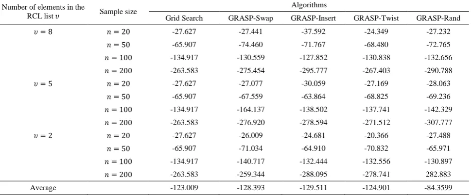
TABLE 4. Log-likelihood values for example 4 with (𝛼, 𝛽, 𝛿) = (8, 9, 2)
Number of elements in the
RCL list 𝜐 Sample size
Algorithms
Grid Search GRASP-Swap GRASP-Insert GRASP-Twist GRASP-Rand
𝜐 = 8 𝑛 = 20 -27.627 -27.441 -37.592 -24.349 -27.232
𝑛 = 50 -65.907 -74.460 -71.767 -68.480 -72.765
𝑛 = 100 -134.917 -130.559 -127.852 -130.838 -132.656
𝑛 = 200 -263.583 -275.454 -295.777 -267.403 -290.788
𝜐 = 5 𝑛 = 20 -27.627 -27.077 -30.059 -27.169 -28.063
𝑛 = 50 -65.907 -67.559 -63.864 -68.825 -69.236
𝑛 = 100 -134.917 -164.137 -138.502 -137.741 -142.329
𝑛 = 200 -263.583 -276.920 -278.594 -271.512 -307.777
𝜐 = 2 𝑛 = 20 -27.627 -26.009 -24.681 -20.366 -27.488
𝑛 = 50 -65.907 -71.034 -64.910 -70.832 -65.971
𝑛 = 100 -134.917 -140.717 -132.444 -132.556 -130.897
𝑛 = 200 -263.583 -259.344 -288.095 -278.741 282.883
Average -123.009 -128.393 -129.511 -124.901 -84.3599
When run time violated, the best obtained solution is recorded and its log-likelihood function are reported. Figure 3 shows a simple pseudo-code of grid search algorithm.
The next remaining columns present the value of achieved log-likelihood objective functions by algorithms Swap, Insert, GRASP-Twist and GRASP-Rand respectively. As we expected, the objective function gets negative values which is due to nature of log function for input probabilities between
0 and 1. The aim is to find the value of parameters
(𝛼, 𝛽, 𝛿) with highest value of log-likelihood function.
Since the proposed GRASP algorithms are random based search methods, the way they approaches their final statuses is of interest. In order to further assess the performance of GRASP algorithms, the quality of solutions obtained by algorithms are depicted in sequel. Figure 4 shows the log-likelihood objective functions for average values of log-likelihood objective functions. The grid search is a relatively full enumeration method which is expected to reach better solutions. After that, as can be seen from results, the rank of algorithms in terms of quality of solutions is Rand, GRASP-Twist, GRASP-Swap and GRASP-Insert.
Procedure Grid search 1. Construct grid network;
2. for maximum parameter values (𝛼, 𝛽, 𝛿) are not violated
3. evaluate the current solution point on network;
4. updating process; 7. end
end Grid search
Figure 3. Grid search procedure
Figure 4. The result of comparisons
6. CONCLUSION
The Weibull distribution plays an important role in several real world applications such as reliability and lifetime studies. This issue has attracted many attentions to precise estimation of the Weibull parameters. The estimation of parameters of three-parameter Weibull distribution is intractable analytically. In this research, the GRASP algorithm with four different local search schemes was developed to maximize the log-likelihood function of a three-parameter Weibull distribution. The performance of the suggested algorithms was assessed and compared with the benchmark grid search method. The obtained results supported the appropriate performance of estimations attained in terms of both accuracy and efficiency. As a direction for future research, it is interesting to devise other numerical search methods like other recent metaheuristics and compare the results.
-140 -120 -100 -80 -60 -40 -20 0
7. REFERENCES
1. Tan, Z., "A new approach to mle of weibull distribution with interval data", Reliability Engineering & System Safety, Vol. 94, No. 2, (2009), 394-403.
2. Castet, J.-F. and Saleh, J.H., "Satellite and satellite subsystems reliability: Statistical data analysis and modeling", Reliability
Engineering & System Safety, Vol. 94, No. 11, (2009),
1718-1728.
3. Akdag, S.A. and Dinler, A., "A new method to estimate weibull parameters for wind energy applications", Energy Conversion
and Management, Vol. 50, No. 7, (2009), 1761-1766.
4. Elandt-Johnson, R.C. and Johnson, N.L., "Survival models and data analysis, John Wiley & Sons, Vol. 74, (1999).
5. Marani, A., Lavagnini, I. and Buttazoni, C., "Statistical study of air pollution concentration via generalized gamma", Journal of
the Air Pollution Control Association, Vol. 36, (1986),
1050-1054.
6. Garcia-Pascual, P., Sanjuan, N., Melis, R. and Mulet, A., "Morchella esculenta (morel) rehydration process modelling",
Journal of Food Engineering, Vol. 72, No. 4, (2006), 346-353.
7. Diaconu, A., "Weibull distribution as a model for growth/decline in product sales", Metalurgia International, Vol. 14, (2009), 184-185.
8. Arenas, J.M., Narbon, J.J. and Alia, C., "Optimum adhesive thickness in structural adhesives joints using statistical techniques based on weibull distribution", International
Journal of Adhesion and Adhesives, Vol. 30, No. 3, (2010),
160-165.
9. Dodson, B., "The weibull analysis handbook, ASQ Quality Press, (2006).
10. Qiao, H. and Tsokos, C.P., "Estimation of the three parameter weibull probability distribution", Mathematics and Computers
in Simulation, Vol. 39, No. 1-2, (1995), 173-185.
11. Nosal, M. and Nosal, E., "Three-parameter weibull generator for replacing missing observations", in meeting of the international conference on statistics and related fields., (2003).
12. Teimouri, M., Hoseini, S.M. and Nadarajah, S., "Comparison of estimation methods for the weibull distribution", Statistics, Vol. 47, No. 1, (2013), 93-109.
13. Bartolucci, A.A., Singh, K.P., Bartolucci, A.D. and Bae, S., "Applying medical survival data to estimate the three-parameter weibull distribution by the method of probability-weighted moments", Mathematics and Computers in Simulation, Vol. 48, No. 4, (1999), 385-392.
14. Bartkute, V. and Sakalauskas, L., "The method of three-parameter weibull distribution estimation", Actaet
Commentationes Universitatis Tartuensis de Mathematica,
Vol. 12, (2008), 65-78.
15. Jukic, D., Bensic, M. and Scitovski, R., "On the existence of the nonlinear weighted least squares estimate for a three-parameter weibull distribution", Computational Statistics & Data
Analysis, Vol. 52, No. 9, (2008), 4502-4511.
16. Jukic, D. and Markovic, D., "On nonlinear weighted errors-in-variables parameter estimation problem in the three-parameter weibull model", Applied Mathematics and Computation, Vol. 215, No. 10, (2010), 3599-3609.
17. Marković, D. and Jukić, D., "On nonlinear weighted total least squares parameter estimation problem for the three-parameter weibull density", Applied Mathematical Modelling, Vol. 34, No. 7, (2010), 1839-1848.
18. Gove, J.H., "Moment and maximum likelihood estimators for weibull distributions under length-and area-biased sampling",
Environmental and Ecological Statistics, Vol. 10, No. 4,
(2003), 455-467.
19. Jaruskova, D., "Maximum log-likelihood ratio test for a change in three parameter weibull distribution", Journal of Statistical
Planning and Inference, Vol. 137, No. 6, (2007), 1805-1815.
20. Chang, T.P., "Performance comparison of six numerical methods in estimating weibull parameters for wind energy application", Applied Energy, Vol. 88, No. 1, (2011), 272-282. 21. Nagatsuka, H., Kamakura, T. and Balakrishnan, N., "A
consistent method of estimation for the three-parameter weibull distribution", Computational Statistics & Data Analysis, Vol. 58, (2013), 210-226.
22. Luus, R. and Jamme, M., "Estimation of parameters in 3-parameter weibull probability distribution functions",
Hungarian Journal of Industry and Chemistry, Vol. 33, No.
1-2, (2005).
23. Ismail, A.A., "Estimating the parameters of weibull distribution and the acceleration factor from hybrid partially accelerated life test", Applied Mathematical Modelling, Vol. 36, No. 7, (2012), 2920-2925.
24. Abbasi, B., Jahromi, A.H.E., Arkat, J. and Hosseinkouchack, M., "Estimating the parameters of weibull distribution using simulated annealing algorithm", Applied Mathematics and
Computation, Vol. 183, No. 1, (2006), 85-93.
25. Abbasi, B., Rabelo, L. and Hosseinkouchack, M., "Estimating parameters of the three-parameter weibull distribution using a neural network", European Journal of Industrial Engineering, Vol. 2, No. 4, (2008), 428-445.
26. Abbasi, B., Niaki, S.T.A., Khalife, M.A. and Faize, Y., "A hybrid variable neighborhood search and simulated annealing algorithm to estimate the three parameters of the weibull distribution", Expert Systems with Applications, Vol. 38, No. 1, (2011), 700-708.
27. Wang, F.-K., "Using bbpso algorithm to estimate the weibull parameters with censored data", Communications in
Statistics-Simulation and Computation, Vol. 43, No. 10, (2014),
2614-2627.
28. Moeini, A., Jenab, K., Mohammadi, M. and Foumani, M., "Fitting the three-parameter weibull distribution with cross entropy", Applied Mathematical Modelling, Vol. 37, No. 9, (2013), 6354-6363.
29. Yang, F. and Yue, Z., "Kernel density estimation of three-parameter weibull distribution with neural network and genetic algorithm", Applied Mathematics and Computation, Vol. 247, (2014), 803-814.
30. Okcu, H.H., Aksoy, E. and Dogan, M.I., "Estimating the parameters of 3-p weibull distribution through differential evolution", Applied Mathematics and Computation, Vol. 251, (2015), 211-224.
31. Okcu, H.H., Ozsoy, V.S., Aksoy, E. and Dogan, M.I., "Estimating the parameters of 3-p weibull distribution using particle swarm optimization: A comprehensive experimental comparison", Applied Mathematics and Computation, Vol. 268, (2015), 201-226.
32. Cousineau, D., "Fitting the three-parameter weibull distribution: Review and evaluation of existing and new methods", IEEE
Transactions on Dielectrics and Electrical Insulation, Vol. 16,
No. 1, (2009), 281-288.
33. Lehman, E.H., "Shapes, moments and estimators of the weibull distribution", IEEE Transactions on Reliability, Vol. 12, No. 3, (1963), 32-38.
34. White, J.S., "The moments of log-weibull order statistics",
Technometrics, Vol. 11, No. 2, (1969), 373-386.
35. Bain, L.J. and Antle, C.E., "Estimation of parameters in the weibdl distribution", Technometrics, Vol. 9, No. 4, (1967), 621-627.
Fitting the Three-parameter Weibull Distribution by using Greedy Randomized
Adaptive Search Procedure
H. Mokhtaria, A. Salmasniab
a Department of Industrial Engineering, Faculty of Engineering, University of Kashan, Kashan, Iran
b Department of Industrial Engineering, Faculty of Engineering and Technology, University of Qom, Qom, Iran
P A P E R I N F O
Paper history:
Received 29 August 2016
Received in revised form 01 January 2017 Accepted 09 February 2017
Keywords: Statistical Inference Weibull Distribution
Greedy Randomized Adaptive Search Procedures
Grid Search
ديكچ ه
هدرتسگ روط هب لوبیاو عیزوت یم رارق هدافتسا دروم یسدنهم فلتخم تاعوضوم رد یا
گ رایسب عیزوت کی هکارچ ،دری
یگژیو عیزوت نیا هولاع هب .تسا عونتم لاکشا اب فطعنم یم رب رد زین ار عیزوت عباوت زا یرگید دادعت یاه
نکیلو .دریگ
هدافتسا ناکم رتماراپ و لکش رتماراپ ،سایقم رتماراپ ینعی نآ رتماراپ هس قیقد نیمخت مزلتسم عیزوت نیا زا زیمآ تیقفوم ی
شلات هلاسم نیا .تسا تمس هب ار اه
شور هعسوت یتخس .تسا هداد قوس عیزوت نیا یاهرتماراپ قیقد دروآرب تهج ییاه
.تسا فورعم هدیچیپ ًلاماک دنیآرف کی ناونع هب دنتسه لوهجم هس ره هکینامز ًاصوصخم لوبیاو عیزوت یاهرتماراپ نیمخت
شور ینعی یتابساحم درکیور کی هعلاطم نیا ،ورنیا زا وجتسج
ی قابطنا ی فداصت ی رح ی اص هن یلحم یوجتسج یدادعت اب
یم داهنشیپ ار اهدروآرب تیفیک یاقترا روظنم هب یگیاسمه تیفیک یبایزرا تهج یتابساحم شیامزآ یدادعت نینچمه .دیامن
هکبش یوجتسج متیروگلا اب هسیاقم رد اهدروآرب .دندش ارجا یا