-

Relation between Seismic Moment M

and

Surface Wave Magnitude M

M. Rezapour

and R.G. Pearce

1

Institute of Geophysics, Tehran University, Tehran, Islamic Republic of Iran 2

Department of Geology and Geophysics, University of Edinburgh, West Mains Road, Edinburgh, EH9 3JW, U.K.

Abstract

The relation between

M

and log

M

is examined using Harvard CMT

M

, with

both

M

and the improved surface wave magnitude scale

t S

M

[1] applied to

ISC data. Although

M

shows less scatter than

M

, neither dataset supports a

slope of

M

against log

M

which tends to 1.0 towards smaller magnitudes. Instead,

a good linear fit of slope 0.76 using

M

is found throughout the fitted range of

M

(2.0×10

to 1.26×10

dyne-cm), and this linearity extends down to

M

=2.5×10

dyne-cm. This suggests that previous proposals that

M

data support

a theoretical slope of 1.0 in the low range of magnitude which may be expected

from established relationships, is not justified.

Keywords: Magnitude; Surface wave; Seismic moment; ISC

*

E-mail: rezapour@ut.ac.ir

Introduction

The objective of this article is to reassess the empirical relationship between surface-wave magnitude MS and seismic moment M0. This study was prompted

by the introduction of a surface wave magnitude scale with improved distance correction (MSt ) [1]. Magni-tude, especially MS, as a measure of earthquake strength,

forms a basic dataset in seismology. However there is evidence of bias [2] in published M0 as Central Moment

Tensor (CMT) solutions, nowadays seismologists consider the seismic moment as a more reliable measure of earthquake size. Seismic moment is in theory a direct measure of earthquake size, whereas all magnitude scales are empirical. MS is available for most significant

earthquakes since about third decay of the twentieth century and some historical earthquakes, whereas

routine estimates of M0 by the Harvard group are

only available since about 1977 for earthquakes having body-wave magnitude mb of about 5 and greater.

Therefore development of a reliable relationship between magnitude and seismic moment is of fundamental importance for integrating historical data into earthquake catalogues.

Most global agencies such as the International Seismological Centre (ISC) and the National Earth-quake Information Center of the US geological survey (NEIC) routinely determine MS using an empirical

formula, the so-called “Prague formula” or “IASPEI formula” (International Association of Seismology and Physics of the Earth's Interior), given by

Pr

log( )_max 1.66 log 3.3 S

A ague

M

T

where A is half the peak-to-peak amplitude (on vertical component or resultant amplitude on two horizontal components) in microns, T is the wave period in seconds, and ∆ is the epicentral distance in degrees [3]. Rezapour and Pearce [1] considered the theoretically-known contribution of dispersion and geometrical sprea-ding, and introduced a modified MS formula given by

1

log( ) log∆

max ₃

1

log(sin∆) 0.0046∆ 5.370, 2

A t

M

s = _T +

+ + +

(2)

They concluded that the Μ_st formula gives reduced bias for MS in comparison with the Prague formula, and

that there is less scatter in logM0 for a given M0 when

t s

Μ is used. Ekström and Dziewonski [4], here referred to as ED88, presented evidence of systematic variations in MS due to tectonic setting; they also fitted an

analytical relationship to the MS versus logM0 values.

In the CMT Catalogue the prime location information is that of the NEIC PDE (Preliminary Determination of Epicenters). Here the NEIC epicentral location and origin time (in the ISC Bulletin) were compared with those in the CMT Catalogue. Those epicentral estimates whose absolute values of differences are ≤0.2 degree in both latitude and longitude and absolute value of differences in origin times are ≤5 seconds are assumed to be the same earthquake. 6,553 earthquakes with available MS and M0

were selected in this way, for the time period from 1978 to 1993.

In this paper the relationship between seismic moment M0 and two MSscales, MS ague

Pr

(ISC) and Μ_st are compared using M0 values obtained from the CMT

Catalogue for the above dataset and the conclusions of ED88 are reexamined.

Analysis

Earliest studies have assumed a linear relation between surface-wave magnitude and the log of seismic moment. Under the hypothesis of constant stress drop, theoretical models predict that logM0 and MS are indeed

related linearly:

0

logM = +A BM_S , (3)

The slope (B) commonly found in the literature [5-10] is around 1.5. However, the data and the range of magnitudes used by different authors were slightly different. An attempt to obtain a relation between

magnitude and seismic moment [7,11] resulted as:

0 2

log 10 73

3 S

M = M − . , (4)

where M0 is seismic moment in dyne-cm. The

relationship between seismic moment and earthquake energy is simplified by the observation that the stress drop is quite similar for virtually all earthquakes of magnitudes exceeding about 3. A constant stress drop in low-magnitude seismic data has been reported from a deep borehole [12]. For dataset containing smaller and large earthquakes, has been showed that earthquakes are self-similar over magnitude range M~-2 to ~8 [12]. Other seismologists for smaller earthquakes all from the same region reported that stress drop appears to increase with increasing moment for earthquakes below a critical size about 2.0×1020 dyne-cm, becoming constant for earthquakes larger than critical size [13].

The seismic moment represents the size of an earthquake only at a period much longer than the source process time (~source dimension / shear velocity), so it represent long-period end of the source spectrum [14]. For very large earthquake the corner frequency can fall below ~0.05 Hz (which used for MSdetermination). In

equation (4) because a theoretical slope of 1.0 is only predicted from instantaneous moment release on source rupturing surface, a different slope is to be expected for real data. Moreover, it has been argued [5,15] that the slope should decrease towards larger magnitude on account of the decreasing corner frequency, since the magnitude estimates are derived at a standard frequency.

ED88 chose to use a two-segment linear model, with a quadratic transition between the segments, to fit the global Ms versus logM0 data. They attempted to fit the

averaged magnitude estimates for 2,341 earthquakes, to a hypothesized MS:logM0 relation. In their analytical

relation between MS (as the dependent variable) and

logM0 (as the independent variable) they imposed a

slope of unity for small events, and ₃2 _{for moderate to} large events.

We use the above dataset of 6,553 earthquakes between 1978 and 1993. Magnitudes ( ague

S

ΜPr

and Μt_s) have been recomputed from amplitude and period measurements in the ISC Catalogue to two decimal places, and corresponding M0 values are taken from the

CMT Catalogue. The individual data are plotted in Figures 1a and 1b for ague

S

ΜPr

and Μt_s respectively. The event magnitudes are averaged within each 0.1-wide interval of logM0 units, and are plotted in Figures

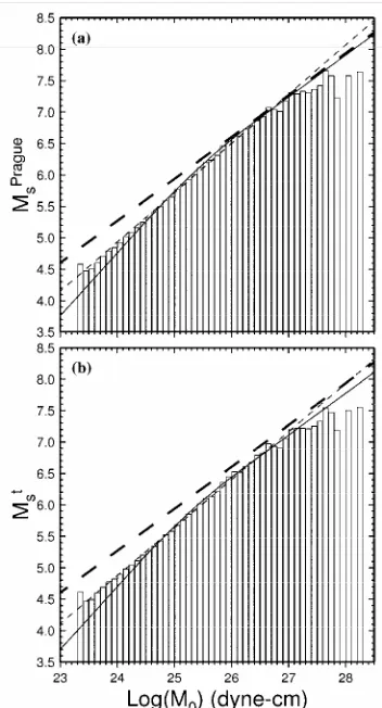
Figure 1. Distribution of Ms values against logM0 for individual data points 6,553. (a) for Μ_SPrague values. (b) for

t S

Μ values. The relationship of Hanks and Kanamori [7] (our Equation 4) is shown by a thick dashed line in both graphs.

There are some minor differences between this dataset (6,553 selected earthquakes) and that of ED88 resulting from their use of NEIC rather than ISC data. They used ΜSNEIC values from events for which both hNEIC and hCMT are less than 50 km, whereas here data from events with hISC≤ 60 km are used. Also, their data window was 1977-1987 whereas here 1978-1993 is used (consistent ISC MS determination began in 1978).

Although we use the same lower M0 limit of 2.0×1024

dyne-cm for fitting, because of saturation a more restrictive upper limit of M0=1.26×1027 dyne-cm is

imposed, it seems the saturation in this dataset appears at this value. However, increasing the number of broad-band and very broad-broad-band seismic stations all over world and using surface wave measurements from these station without the IASPEI restriction in period to MS

determination cases the saturation occurs at grater value.

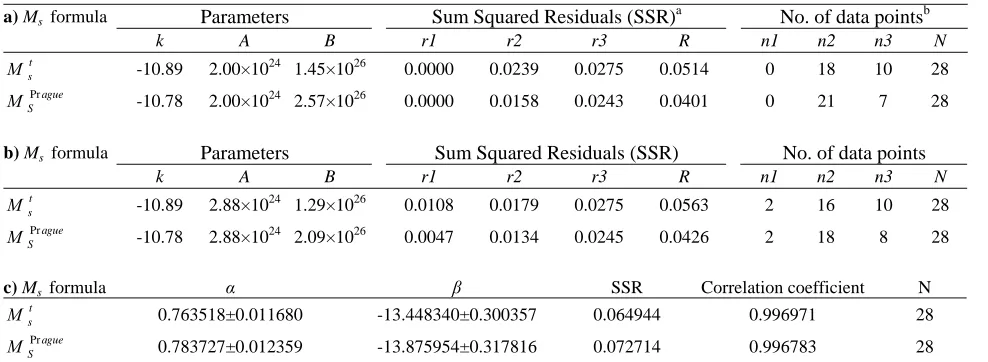
Figure 2. Average M_Svalues over 0.1-unit-wide intervals of logM0. (a) for

Prague S

Μ values. (b) for Μ_st values. In (a) and (b) the solid curve represents the ED88’s analytical relation (their Eq. 2) and our Eq. (6) respectively, and the thin dashed line shows the linear regression fit to the same data. In (a) and (b) the thick dashed line shows the relationship of Hanks and Kanamori [7]. In (a) and (b) the range of data used in the fits is highlighted in gray.

The analytic relation has three free parameters and is most easily represented using the formulation of ED88, except that we control the limits of the segments by constants A and B in units of M0 (rather than logM0), in

order to relate the constants to the graph more easily. We obtain

0 0

(logA logB)

k log for A

6 S

M = − + + M M < (5a)

0

2 0

0 (log A log B)

k logM

6

(log log A)

for A B

6(log B log A) S

M

M

M

+

= − +

−

− ≤ ≤

−

Table 1. Fitting parameters obtained when applying the analytical relation of Eqs. (5a, 5b, 5c) to the Μ_SPrague and Μ_st datasets. a) Without a constraint of a segment with a slope of 1.0. b) Considering a minimum of two points are required to lie along a slope of 1.0. c)For applying a linear relation of Μ_s =αlogM₀ +β

a) Ms formula Parameters Sum Squared Residuals (SSR)a No. of data pointsb

k A B r1 r2 r3 R n1 n2 n3 N

t s

Μ -10.89 2.00×1024 1.45×1026 0.0000 0.0239 0.0275 0.0514 0 18 10 28 Prague

S

Μ -10.78 2.00×1024 2.57×1026 0.0000 0.0158 0.0243 0.0401 0 21 7 28

b) Ms formula Parameters Sum Squared Residuals (SSR) No. of data points

k A B r1 r2 r3 R n1 n2 n3 N

t s

Μ -10.89 2.88×1024 1.29×1026 0.0108 0.0179 0.0275 0.0563 2 16 10 28 Prague

S

Μ -10.78 2.88×1024 2.09×1026 0.0047 0.0134 0.0245 0.0426 2 18 8 28

c) Ms formula α β SSR Correlation coefficient N

t s

Μ 0.763518±0.011680 -13.448340±0.300357 0.064944 0.996971 28

Prague S

Μ 0.783727±0.012359 -13.875954±0.317816 0.072714 0.996783 28

a

r1, r2, and r3, are respectively the Sum of the Squared Residuals of the three sections of the relationship in Eqs. (5a, 5b, 5c), and R is that for the total relation.

b

n1, n2, n3, and N are the number of data points used to compute the four SSR values, respectively.

0 0

2

k log for B

3 S

M = + M M > (5c)

We first attempt to fit an analytical function of the form proposed by ED88 using t

S

Μ . The results of our analysis are shown in Table 1. Table-1a shows the resulting fit when the Sum of the Squared Residuals (SSR) is minimized in k, A and B using ΜSt and the specified range of M0. It is seen that A is equal to

2.0×1024 dyne-cm, which corresponds to the lower limit of the fitted range. Hence, no segment with a slope of 1.0 remains when the least-squares fit to the functions in Eqs. (5a,5b,5c) is optimized. The full relation is given by

24

0 0

19 30 log for 2 0 10

t S

M = − . + M M < . × (6a)

2

0 0

24 26

0

19.30 log 0.09(log 24.30)

for 2.0 10 1.45 10

t S

M M M

M

= − + − −

× ≤ ≤ × (6b)

26

0 0

2

10 89 log for 1 45 10

3 t

S

M = − . + M M > . × (6c)

We next reassess the fit to Eqs. (5a,5b,5c) using ague

S

ΜPr

(Table-1a). Again we see that no segment of slope 1.0 remains, although the SSR is smaller than when ΜSt values are used.

The above results suggest that the observed data for t

S

Μ and even ΜS ague Pr

do not provide evidence of a slope of unity for earthquakes in the relationship between Ms and logM0. If a minimum of two points are

required to lie along a slope of 1.0 (Table-1b), then for ague

S

ΜPr

the values of k, A, and B are almost equivalent to those given by ED88.

The analytical relation of ED88 (their Eq. 2) and our fit (our Eqs. 6a, 6b, 6c) are plotted with solid curves, and the relationship of Hanks and Kanamori [7] is shown by a thick dashed line (Figs. 2a, 2b). Dark histogram bars are used to highlight the range of data used to compute the fit. These plots show visually that the evidence in support of the analytical relation proposed by ED88 is even weaker when the improved

t s

Μ scale is used. But by using a standard linear

regression a better fit is obtained for Μ_st than for ague

S

ΜPr

as shown by thin dashed lines (Figs. 2b, 2a). It is important to compare the success of testing different hypotheses. First, the sum squared residuals of fit in the both hypotheses using Μ_st scale are compared with residuals of fit using ague

S

ΜPr

scale. Comparison shows that the residuals in the case of applying analytical relation and using Μ_st values is larger than that for using ΜS ague

Pr

the case of fitting a single linear regression (compare fitting parameters in Table-1b and Table-1c). For both

ague S

ΜPr

and Μt_s the residuals of fit is increased when a standard linear regression is applied. This is expected, because multiple linear and unlinear regressions analyze normally gives smaller residuals than only one single linear regression. The residuals of a single fit by using

t s

Μ values about 11% is reduced in comparison with using ague

S

ΜPr

values. Moreover, it is apparent (Figs. 2a, 2b) that a linear fit extends to smaller moments which were excluded from the fit because of possible incompleteness of earthquake catalogue, and also because of possible upward bias in Msvalues close to

the detection threshold. We use the same lower M0 limit

of 2.0×1024 dyne-cm for fitting as ED88 used. It is apparent that the goodness of fit strongly depends on the upper limit of fitted data, because the progressively smaller number of earthquakes towards higher moment create greater scatter, and because of the onset of magnitude saturation.

ED88’s main reason for imposing a lower limit of 2.0×1024 dyne-cm when fitting their relation was the upward biasing of Ms Values caused by station

threshold effects. Of course, this specific source of bias is governed by the bias in magnitude rather than moment. Figures 1a and 1b show a large scatter in the logM0: Ms: relation for individual events, particularly at

smaller magnitude. If data points below, say Ms=4.5 are

affected by station threshold bias, then this would have only a marginal effect on Figures 2a and 2b. We conclude that this source of bias does not contribute significantly to histograms with logM0 > 23.4 (M0 >

2.5×1023 dyne-cm).

To examine the possible upward bias in low magnitude values we determined station correction (average Sstation

event S M

M − values for each station) by using data of 10,894 earthquakes for which three or more observations have been used in the calculation of ISC

S

Μ . The average station correction in 0.1-unit-wide ranges of logM0 against logM0, and the histograms of

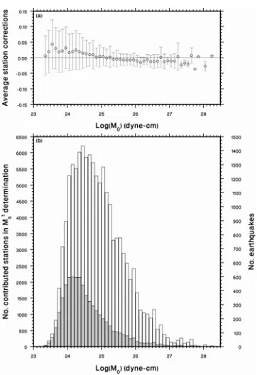
used data are plotted respectively in Figures 3a and 3b for 6,553 earthquakes. Figure 3a shows that earthquakes with M0 smaller than ~1025 dyn-cm have been reported

by individual stations in which most of station corrections (M_Sevent −M_Sstation) are positive. Therefore, by applying station correction, calculated MS values will be increased about 0.1 for earthquakes with M0 smaller than ~1025 dyn-cm, this means the dataset used in this study does not show an upward bias in low magnitude values.

We conclude that data used here are more consistent with a linear fit than with the more complicated analytic relation of Eqs. (5a, 5b, 5c), and that this is so over the wider moment range from M0=2.5×1023 to

M0=1.26×1027 dyne-cm, however in our analysis we

used data range from 2.0×1024 to 1.26×1027 dyne-cm. This conclusion implies that logM0 is proportional to

about 1.3MSover this wider magnitude range or MS is

proportional to logM0 as:

0 (0.763518 0.011680) log

(13.448340 0.300357), t

S

M = ± M

− ± (7)

The observed linear relationship suggests that the spectral fall-off above the corner frequency is not influencing Ms measurements at least up to MS ≤7.2. We can only speculate on the origin of the 0.76 gradient. We can be confident that it is not caused by inadequate distance correction since we are using Μt_S (Table 1c) although the difference between this value and the 0.78 obtained for ague

S

ΜPr

(Table 1c) may represent such an effect. One possibility is that the deviation of our gradient from 1.0 represents a dependence of stress drop ∆σ upon M0. If this were so, a

relation ∆σ ∝M₀0.14is implied, which corresponds to a reduction in stress drop towards larger earthquakes.

The generation of 20-second surface-wave used in the MS calculation depends on focal depth, focal

mechanism as well as on the earth structure near the earthquake source or along the propagating path. In order to compare the focal mechanism effect on estimated MS, the data are grouped. Here, following

Frohlich and Apperson [17], earthquakes are grouped according to dip angle values of their P, B and T axes (δP, δB, and δT values) which were taken from Harvard source solutions. The mechanism is considered as strike-slip or normal faulting when dip angle of the B or P axes exceeds 60° respectively. When the T axis exceeds 50° the mechanism is proposed as thrust faulting. The Μ_St values for each group averaged over 0.1-unit-wide intervals of logM0 are plotted in Figure 4.

This figure represents a set of (Μt_S, logM0) regression

lines over a wide range of M0 (2.5×1023 to 1.26×1027

than of the other lines. Consequently, in the case of normal earthquakes, for a fixed value of M0>~1025, the

magnitude Μ_St would be small (~ 0.1) in comparison with other earthquakes.

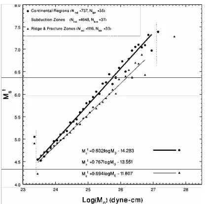
To compare average Μ_St in different tectonic settings defined as “oceanic ridges & fracture zones”, “continental”, and “subduction zones”, the data were classified using Flinn-Engdahl seismic region number [16], and Μ_St values were averaged over 0.1-wide intervals of logM0. In Figure 5 average MSversus logM0

are compared for different tectonic regions. This figure shows that the continental earthquakes have a larger

t S

Μ than corresponding earthquakes along mid-oceanic ridges and subduction zones with the same seismic moment. However, the largest earthquakes occur in subduction zones. For a given M0 value, mid- oceanic

ridge earthquakes have a smaller Μ_St than earthquakes in other regions. The difference between these regions is not constant and it increases with increasing seismic moment. Also, the number of individual data points controls the scatter of averaged data.

Figure 3. (a) Average station corrections of 111,555 station records for 6,553 earthquakes over 0.1-wide intervals of logM0 against logM0. Error bars show a standard deviation of data points. (b) Histograms of dataset used in this study. White and gray histograms represent respectively number of contributed stations and earthquakes.

Conclusions

In the relation of MS with logM0 the observed data do

not provide evidence of a slope of unity towards smaller events when either the Μt_S or ΜS ague

Pr

scales are used.

A simple linear regression gives a slope of 0.76 for Μt_S over a wide range of moments from 2.0×1024 to 1.26×1027 dyne-cm extending below the range used for fitting. The linear regression is less good for ague

S

ΜPr . It is concluded that a linear fit of gradient 0.76 is preferable to the analytical relation of Eqs. (5a, 5b, 5c), making logM0 proportional to about 1.3MS over this

wider moment range. Comparison of (Μ_St , logM0)

relations for earthquakes with different focal mechanism do not show a very significant differences, but, the (Μ_St , logM0) relation for different tectonic settings

shows a systematic bias.

Figure 5. Average M_St over 0.1-wide intervals of logM0 against logM0 in different tectonic regions. The filled circles, squares and triangles represent the average magnitude for earthquakes in “continental”, “subduction zones” and “oceanic ridges and fracture zones” respectively. The thick solid line, gray and thin solid lines represent linear regression lines to the data points in “continental”, “subduction zones” and “oceanic ridges & fracture zones” respectively. For regression analysis only the data points in the seismic moment range 2.5×1023 to 1.26×1027 dyne-cm were used which marked by vertical dotted lines. Nind and Nbin represent the number of individual and the relevant binned data points, respectively.

Acknowledgments

We thank Prof A. Douglas, and Drs I. Main and D. Bowers for their valuable comments that improved this manuscript. We also thank anonymous reviewers, for their useful reviews. Funding from the Research Council of the University of Tehran is greatly appreciated. The figures were prepared using Generic Mapping Tools [18].

References

1. Rezapour M. and Pearce R.G. Bias in surface wave magnitude Ms due to inadequate distance corrections.

Bull. Seism. Soc. Am., 88: 43-61 (1998).

2. Patton H.J. Bias in the centroid moment tensor for central Asian earthquakes: Evidence from regional surface wave data. J. Geophys. Res., 103: 26, 963-26, 974 (1998). 3. Vaněk J., Zatopek A., Karnik V., Kondorskaya N.V.,

Riznichenko Y.V., Savarensky E.F., Solov'ev S.L., and Shebalin N.V. Standardization of magnitude scales. Bull. Acad. Sci. USSR, Geophys, Ser. (English Transl.) No. 2, 108-111 (1962).

4. Ekström G. and Dziewonski A.D. Evidence of bias in estimations of earthquake size. Nature, 332: 319-323 (1988).

5. Kanamori H. and Anderson D. Theoretical basis of some empirical relations in seismology. Bull. Seism. Soc. Am.,

65: 1073-1095 (1975).

6. Purcaru G. and Berckhemer H. A magnitude scale for very large earthquakes. Tectonophysics, 49: 189-198 (1978).

7. Hanks T.C. and Kanamori H. A moment magnitude scale.

J. Geophys. Res., 84: 2348-2350 (1979).

8. Caputo M. and Console R. Statistical distribution of stress drops and faults of seismic regions, Tectonophysics, 67: T13-T20 (1980).

9. Hyndman R.D. and Weichert D.H. Seismicity and rates of relative motion on the plate boundaries of Western North America. Geophys. J. R. Astr. Soc., 72: 59-82 (1983). 10. Dziewonski A.M. and Woodhouse J.H. An experiment in

systematic study of global seismicity: Centroid-moment tensor solutions for 201 moderate and large earthquakes of 1981. J. Geophys. Res., 88: 3247-3271 (1983).

11. Kanamori H. The energy release in great earthquakes.

Ibid., 82: 2981-2987 (1977).

12. Abercrombie R. and Leary P. Source parameters of small earthquakes recorded at 2.5 km depth, Cajon Pass, southern California: implications for earthquakes scaling.

Geophys. Res. Lett., 20: 1511-1514 (1993).

13. Shi J., Kim W., and Richards P.G. The corner frequencies and stress drops of intraplate earthquakes in the northeastern United States. Bull. Seism. Soc. Am., 88: 531-542 (1998).

14. Kanamori H. Magnitude scale and quantification of earthquakes. Tectonophysics, 93: 185-199 (1983).

15. Aki K. Scaling law of seismic spectrum. J. Geophys. Res.

72: 1217-1231 (1967).

16. Flinn E.A., Engdahl E.R., and Hill A.R. Seismic and geographical regionalization. Bull. Seism. Soc. Am., 64: 771-993 (1974).

17. Frohlich C. and Apperson K.D. Earthquake focal mechanism, moment tensors, and the consistency of seismic activity near plate boundaries. Tectonics, 11: 279-296 (1992).

18. Wessel P. and Smith W.H.F. New version of the Generic Mapping Tools released. EOS Trans. Amer. Geophys., U.