ESTIMATION OF NETWORK RELIABILITY FOR A FULLY
CONNECTED NETWORK WITH UNRELIABLE NODES AND
UNRELIABLE EDGES USING NEURO OPTIMIZATION
D. Bhardwaj
Department of Computer Science, GLA Institute of Technology and Management P.O. Box 281406, Mathura, India
S.K. Jain and Manu Pratap Singh*
Department of Computer Science, ICIS, Dr. B.R. Ambedkar University P.O. Box Agra-282002, Uttar Pradesh, India
[email protected] - [email protected] *Corresponding Author
(Received: September 18, 2008 – Accepted in Revised Form: February 19, 2009)
Abstract In this paper it is tried to estimate the reliability of a fully connected network of some unreliable nodes and unreliable connections (edges) between them. The proliferation of electronic messaging has been witnessed during the last few years. The acute problem of node failure and connection failure is frequently encountered in communication through various types of networks. We know that a network can be defined as an undirected graph N(V,E). It is believed that in a network the nodes as well as the connections can fail and hence can cause unsuccessful communication. So, it is important to estimate the network reliability to encounter the network failure. Various tools have been used to estimate the reliability of various types of networks. In this paper we are considering the approach of neuro optimization for estimating the network reliability. We use the simulation annealing to estimate the probabilities of various nodes in the network and Hopfield model to calculate the energies of these nodes at various thermal equilibriums. The state of the minimum energy represents the maximum reliability state of the network.
Keywords Network Reliability, Neural Optimization, Simulated Annealing, Hopfield Model
ﻩﺪﻴﻜﭼ
ﺍ ﺭﺩ ﻳ ﻠﺑﺎﻗﺎﺗ ﻩﺪﺷﺵﻼﺗ ﻪﻟﺎﻘﻣ ﻦ ﻴ
ﻤﻃﺍ ﺖ ﻴ ﻥﺎﻨ ﻳ ًﻼﻣﺎﮐ ﻪﮑﺒﺷ ﮏ ﭘ
ﻴ ﺩﺍﺪﻌﺗ ﻞﻣﺎﺷﻪﮐﻪﺘﺳﻮ ﻱ ﻏ ﻩﺮﮔ ﻴ ﻞﺑﺎﻗﺮ ﻤﻃﺍ ﻴ ﺕﻻﺎﺼﺗﺍﻭﻥﺎﻨ ) ﻪﺒﻟ ﺎﻫ ﻱ ( ﻏﻴ ﻤﻃﺍﻞﺑﺎﻗﺮ ﻴ ﺑﻥﺎﻨ ﻴ ﺍﻦ ﻳ ﻩﺮﮔﻦ ﻣﺎﻫ ﻲ ﻤﺨﺗ،ﺪﺷﺎﺑ ﻴ
ﺩﻮﺷﻩﺩﺯﻦ . ﻝﺎﺳﺭﺩ ﺎﻫ ﻱ ﺧﺍ ﻴ ﺪﻫﺎﺷ،ﺮ ﺍﺰﻓﺍ ﻳ ﺮﺳﺶ ﻳ ﭘﻝﺎﺳﺭﺍﻊ ﻴ ﻡﺎ ﺎﻫ ﻱ ﻧﻭﺮﺘﮑﻟﺍ ﻴ ﮑ ﻲ ﻩﺩﻮﺑ ﺍﻳ ﻢ . ﺭﺩ ﻪﮑﺒﺷ ﺎﻫ ﻱ ﻩﺮﮔﺖﻓﺍﺩﺎﺣﻞﮑﺸﻣ،ﻒﻠﺘﺨﻣ ﺕﻻﺎﺼﺗﺍﺖﻓﺍﻭﺎﻫ
ﻩﺩﺎﺘﻓﺍﻕﺎﻔﺗﺍﺕﺎﻌﻓﺩﻪﺑ ﺖﺳﺍ . ﻣ ﻲ ﻧﺍﺩ ﻴ ﻪﮐﻢ ﻳ ﻣﺍﺭﻪﮑﺒﺷﮏ ﻲ
ﻏﺭﺍﺩﻮﻤﻧﺕﺭﻮﺻﻪﺑﻥﺍﻮﺗ ﻴ ﻘﺘﺴﻣﺮ ﻴ ﻢ N(V,E) ﺮﻌﺗ ﻳ ﺩﺮﮐﻒ .
ﺍﺮﺑ ﺭﻮﺼﺗ ﻳ
ﺭﺩﻪﮐ ﺖﺳﺍ ﻦ ﻳ
ﻩﺮﮔ،ﻪﮑﺒﺷﮏ ﻣﺕﻻﺎﺼﺗﺍ ﺪﻨﻧﺎﻣ ﻢﻫ ﺎﻫ
ﻲ ﺘﻧ ﺭﺩ ﻭﺪﻧﻮﺷ ﺖﻓﺍﺭﺎﭼﺩ ﺪﻨﻧﺍﻮﺗ ﻴ
ﺚﻋﺎﺑ ﻪﺠ
ﻣﺎﻧﻁﺎﺒﺗﺭﺍ ﺪﻧﺩﺮﮔﻖﻓﻮ .
ﻠﺑﺎﻗﻪﮐﺖﺳﺍﻢﻬﻣﺍﺬﻟ ﻴ
ﻤﻃﺍﺖ ﻴ ﻤﺨﺗﻪﮑﺒﺷﺖﻓﺍﺎﺑﻪﻬﺟﺍﻮﻣﺭﺩﻪﮑﺒﺷﻥﺎﻨ ﻴ ﻩﺩﺯﻦ ﺩﻮﺷ . ﺵﻭﺭ ﺎﻫ ﻱ ﻔﻠﺘﺨﻣ ﻲ ﺍﺮﺑ ﻱ ﻤﺨﺗ ﻴ ﻠﺑﺎﻗ ﻦ ﻴ ﻤﻃﺍ ﺖ ﻴ ﻪﮑﺒﺷﻒﻠﺘﺨﻣ ﻉﺍﻮﻧﺍ ﻥﺎﻨ ﻪﺑ ﺎﻫ
ﺭﺎﮐ ﺖﺳﺍﻩﺪﺷ ﻩﺩﺮﺑ .
ﺍ ﺭﺩ ﻳ ﻭﺭﺎﻣ ،ﻪﻟﺎﻘﻣ ﻦ ﻳ ﺩﺮﮑ ﻬﺑ ﻴ ﻪﻨ ﺯﺎﺳ ﻱ ﺒﺼﻋ ﻲ ﺍﺮﺑﺍﺭ ﻱ ﻤﺨﺗ ﻴ ﻠﺑﺎﻗﻦ ﻴ ﻤﻃﺍﺖ ﻴ ﻪﺑ ﻪﮑﺒﺷﻥﺎﻨ ﻩﺩﺮﺑﺭﺎﮐ
ﺍﻳ ﻢ . ﺒﺷﺯﺍﺎﻣ ﻴﻪ ﺯﺎﺳ ﻱ ﺗﺭﺍﺮﺣ ﻲ ﺍﺮﺑ ﻱ ﻤﺨﺗ ﻴ ﻦ
ﻩﺩﺮﮐﻩﺩﺎﻔﺘﺳﺍﻪﮑﺒﺷ ﺭﺩﻩﺮﮔﻉﺍﻮﻧﺍﻝﺎﻤﺘﺣﺍ ﺍﻳ
ﺍﺮﺑ ﻭﻢ ﻱ ﮊﺮﻧﺍ ﻪﺒﺳﺎﺤﻣ ﻱ ﺍ ﻳ ﻩﺮﮔﻦ ﻪﻧﺯﺍﻮﻣﺭﺩﺎﻫ ﺎﻫ ﻱ ﺗﺭﺍﺮﺣ ﻲ ،ﻒﻠﺘﺨﻣ ﭖﻮﻫﻝﺪﻣ ﻓﻴ
ﻪﺘﻓﺮﮔﺭﺎﮐﻪﺑﺍﺭﺪﻠ ﺍﻳ ﻢ . ﻌﺿﻭ ﻴ ﺍﺭﺍﺩِﺖ ﻱ ﺮﺘﻤﮐ ﻳ ﮊﺮﻧﺍﻦ ﻱ ﺮﺗﻻﺎﺑ،ﻦﮑﻤﻣ ﻳ ﻠﺑﺎﻗﻦ ﻴ ﻤﻃﺍﺖ ﻴ ﺩﺭﺍﺩﺍﺭﻪﮑﺒﺷﻥﺎﻨ .
1. INTRODUCTION
In recent years, enormous growth has been seen in electronic message traffic. There is a matching growth of demand in computer and communication networks, both in complexity and size [1]. The
communicate among the nodes in a computer network, so the data can reach successfully to the destination. In other words, it is the probability that the network is in operational state for the given time period [2]. In the network design process, a successful design relies on many factors. Reliability is just one measure of a network that contributes to its overall performance [3]. Hence to achieve the maximum reliability, the nodes and the edges (communication link) both should function properly or with the highest operational probability. The network can become unreliable due to the failure of either node or edge, i.e. failure of networks can cause due to the component failure or communication failure. For example, the routing protocol may fail to recognize a functioning route and hence some data can not reach to the destination, or traffic being concentrated and congested to certain part of network may cause system overload. These are the examples of software and control failure rather than the topological component failures. The topological failure can be categorized as random or non-random. In the network reliability measures we consider the probability of network being operational subject to random failure of its component which includes the nodes failure and communication link failure.
There are various approaches available in the literature to estimate the reliability for the network [4-19]. Almost in every approach, the estimation is based on either the unreliable nodes or edges in the network. Shpungin [20] has proposed a model for estimating the reliability of the network for unreliable nodes and edges as
j m e q j e p )
( r
j !j(m j)! 1
i n v q i v p )
( r
i i!(n i)! 1 )
r ( N
− ∑
π
= −
− ∑
π
= −
=
(1)
Where, pv and pe are the probabilities of the nodes
and edges in up (operational) state and qv, qe are
the probabilities of the nodes and edges in down (non-operational) state, respectively. n and m are number of nodes and the communication links in the network, respectively.
Hence, it is clear from the model of Y. Shpungin [20] that it is the combinatorial approach of estimating the reliability. It is well known that
the combinatorial approach suffers the complexity as the size of the network increases.
of the units and connection strength. The Neural dynamics, in order to search for the global stable state (minimum energy state), may trap in the local minimum of the energy function. Hence, to achieve the global minima, skipping the local minima, the feedback neural network can implement with stochastic units. It is understood that for stochastic unit the state of the unit is updated using a probability law, which is controlled by a temperature parameter (T). Hence at the higher temperature many states are likely to be visited irrespective of the energies of the states. Thus, the local minima of the energy function can be escaped. As the temperature is gradually reduced, the states having lower energies will be visited more frequently. Finally, at T = 0, the state with the lowest energy will have the highest probability. This method of search for a global minimum of the energy function is known as a simulated annealing [26]. In this paper, we are considering a fully connected network. Every node is connected to other nodes, except itself. Some constrains are also employed in the network. The connections between the nodes have been considered in symmetric fashion and the nodes are considered in bipolar states. We have also assumed that the nodes as well as edges of the network may be unreliable, i.e. both nodes and edges can fail. If any node or any edge or both are down (fail), then they are represented with -1 or if they are up (operational) are represented with +1. This network works as the Hopfield type neural network and can be used for optimization. The probabilistic function has used to determine the state update and simulated annealing process has been also employed in order to search the global minimum. The minimum energy states of the network are exhibiting the stability for the network at the given condition. It is quite obvious that as the network becomes more and more stable its reliability will also increase. Thus, in each minimum energy state the network will exhibit some reliability, but the most reliable state of the network may represent with global minimum energy state i.e. the minimum energy state among all the energy minima’s. The proposed method for estimating the network reliability for the given conditions has been implemented with neuro optimization tools and the evolutionary search method i.e. simulated annealing. The following subsections describe the proposed method and its implementation.
2. NETWORK MODEL AND NEURO OPTIMIZATION
The states of the nodes and the communication links between the nodes are described with the undirected graph. Let us consider an undirected graph (or network) N(V,E), where V is set of n vertices (nodes) and E is the set of m edges. Associate with each node x ∈ V and each edge e ∈ E is a bipolar random variable Xε, denoting the operational and
failure state of the edge/node. In particular {Xε=1}
represents the event that the node/edge is up (operational) and {Xε=-1} represents the event that
can be defined as the fully connected network of Mcculloch Pitt’s neuron (processing unit) with the bipolar output state of the units. The output of each unit is fed to all the other units with weight Wij for
all i and j. The weights between the units are considered as the symmetric weights i.e. Wij = Wij
for all i and j. The bipolar output state of each unit can be defined as:
j i ,i all for i n
1 j wijsj )
i x ( f i
s ≠
⎥ ⎥ ⎦ ⎤ ⎢
⎢ ⎣ ⎡
θ − ∑
=
= (2)
and for the convince, θi = 0 (for all i) we have,
j i n
1
j j
s ij w f
i
s ≠
⎥ ⎥ ⎦ ⎤ ⎢
⎢ ⎣ ⎡
∑ =
= (3)
[The state of each unit is either +1 or -1 at any given instant of time]. One of the most successful applications of Hopfield type neural network architecture is in solving the optimization problems [24-27]. An interesting application of the Hopfield network can be observed in a heuristic solution to the NP-complete traveling salesman problem [28]. It is possible to map such type of problem onto a feedback network, where the units and connection strengths are identified by comparing the cost function of the problem with the energy function of the network expressed in terms of the state values of the units and the connection strength as:
ij w j s j i si 2 1
E ∑
≠ −
= (4)
The solution to the problem lies in determining the state of the network at the global minimum of the energy function. In this process it is necessary to overcome the local minima of energy function. This is accomplished by adopting a simulated annealing scheduled for implementing the search for global minimum.
The dynamics of the network by using the bipolar states for each unit can be expressed as:
⎟ ⎟ ⎠ ⎞ ⎜
⎜ ⎝ ⎛
∑ = =
+ n
1 j wijsj(t) sgn
) 1 t ( i
S (5)
Hence, the direct application of the dynamics of
network as specified in Equation 5 in search of a stable state may lead to a state corresponding to a local minimum of the energy function. In order to reach the global minimum, skipping the local minima, the implementation of stochastic unit is required in the activation dynamics of the network. The state of a neural network with stochastic units is described in terms of probability distribution. The probability distribution of the states at thermal equilibrium can be represented as:
T E e z 1 ) S ( P
α − =
α (6)
Where Eα is the energy of the network in the state
Sα and z is the partition function.
The network with stochastic update exhibits the stability on thermal equilibrium at a given temperature (T). Thus, the average value of the state of the network remains constant due to stationary of the probability P(Sα) of the states of
the network at thermal equilibrium. The expected value of the network state can be expressed as:
) S ( P S
S ∑ α
α α >=
< (7)
3. MODELING AND SIMULATION DESIGN
The neural optimization tool with simulated annealing process to ensure the global optimal solution has been employed for estimating the reliability of a network. The network consists of unreliable nodes and edges. This problem has mapped to the neural network of Hopfield type architecture. The unreliable nodes and edges of the network have been considered with processing elements and the connection strength between the process elements in the network. The processing elements exhibit bipolar out put states +1 or -1. It has been considered that if the node of the network is reliable (Operational) then it is in state 1 and the unreliability of the node is exhibited with the state -1. Here, we are representing the network reliability in the form of energy function of the network, which will express in terms of state of the nodes and the connection strength i.e. edges. The objective is to minimize the energy or maximize the reliability of the network by adjusting the network parameters to their optimal values. The dynamics of neural network leads the network towards the stable state, which corresponds to the minimum energy state for the given condition. The global minimum energy state will exhibit the maximum reliability for the network. It is quite obvious that the connection strength or the weights on the edges will be obtained in order to settle the network in the global minimum energy state. Hence, here we employ the Boltzmann learning law for determining the weight for each annealing schedule. The thermal equilibrium has been achieved for each value of the temperature (T) and the probability distribution of the states of the network has been explored for the thermal equilibrium. This process continues until we reached the lower temperature T≈ 0. At this lower temperature value, the network will settle in the global energy minimum state and this will exhibit the maximum reliability state of the network for the given condition. Now, to represent the mathematical modeling of this process we consider a fully connected network with n nodes and 2n edges. At any instant of time one or more nodes or one or more links or both can be down, even though the network remains in operational mode. Thus, it reflects the reliability of the network. In order to determine the global minimum energy state for the network at any given
condition the Hopfield energy function analysis has been used with stochastic activation dynamics. The simulated annealing process with Boltzmann learning rule has been employed for obtaining the optimal weights on edges to explore the global minimum energy state or maximum reliable state for the network. The final optimal values of the weight vector represent the status of operationally for the edges to achieve the reliability for network. A network with stochastic activation dynamics will evolve differently each time it runs, in the sense that the trajectory of the state of the network becomes a sample function of random process. So that, there will never be a static equilibrium or static stable state for the network, instead of this the network can settle in the dynamic equilibrium. In the dynamic equilibrium, the probability distribution of the network states will remain stationary or time independent at a given temperature (T). Thus, the ensemble average of the network states does not change with time. The average of the state can represent in terms of the average value (<Si>) of the output of each unit of the
network i.e.
∫ = >
< Si SiP(Si)dSi (8)
Where P(Si)is the joint probability density function
of state vector Si. The network at the thermal
equilibrium that exhibits the probability of network state is inversely proportional to the energy of the state. Hence, at the higher temperature the higher energy states or less reliable states are more likely to be observed. Now, we reduce the temperature in smaller steps as the annealing schedule and determine the thermal equilibrium for each value of the temperature. It can be observed that as the temperature decreases according to annealing schedule, the probability of visiting the lower energy state increases, and finally the network settle in the global minimum energy state of the network i.e. the state of maximum reliability. To accomplish this process, the weight vector of the network is computed using Boltzmann learning rule as:
] f ij P C ij P [ T ij
W = η −
Δ (9)
Where C ij
network is clamped and f ij
P is the probability of states when the network is running freely. Hence, the weight vector is computed for each annealing schedule till the network does not occupy the global minimum energy state. To speed up the process of simulated annealing, the mean field approximation [29] is used. In this process stochastic update of the bipolar unit is replaced with deterministic analog state.
∑
= >= ∑= < < <
>=
< N
1
j wij Sj
N 1 j i S ij w i
x (10)
Where <xi> the average activation value of the ith
unit and <Sj> represents the expectation of the jth
output state.
Therefore, using the Hopfield energy function analysis and the mean field approximation, we define the expression of energy function for the network of unreliable nodes and edges as:
ij w ) j (S P ) i (S P j i 2 1 j S i S ij w j i 2 1 N E ∑ ∑ − > < > < ∑ ∑ − = (11)
Where <Si> is the expectation of the ith unit at the
present thermal equilibrium (TP) and P(Si) is the
operational probability of the node si.. Let us
consider the kth node in the network which has
been selected at any instant of time for the state updating.
The energy of the network before the update of kth unit can be expressed as:
jk w ) old k S ( P ) old j S ( P j 2 1 ik w ) old k S ( P ) old i S ( P i 2 1 ij w ) old j S ( P ) old i S ( P j i 2 1 old k S old j S j jk w 2 1 old k S old i S
i wik 2 1 old j S old i S jwij i 2 1 old N E ∑ − ∑ − ∑ ∑ − > >< < ∑ − > >< < ∑ − > >< < ∑ ∑ − = (12)
As the kth unit updates its state, the energy function
of the network will change as:
jk w ) new k S ( P ) new j S ( P j 2 1 ik w ) new k S ( P ) new i S ( P i 2 1 ij w ) new j S ( P ) new i S ( P j i 2 1 new k S new j S jwjk 2 1 new k S new i S
i wik 2 1 new j S new i S jwij i 2 1 new N E ∑ − ∑ − ∑ ∑ − > >< < ∑ − > >< < ∑ − > >< < ∑ ∑ − = (13)
Now, the change in energy i.e. Old N New
N E
E
E= −
Δ for
the two different states of the network at the thermal equilibrium should always less than or equal to zero in order to settle the network at global energy minima. Thus, as the network evolve with the new state, the energy of state should either remain same or decreases along the energy landscape as the temperature is reduced as per annealing schedule.
Hence, this process can be formulated as: Old N E New N E
E= −
Δ So that jk w ) Old k S ( P ) Old i S ( P j 2 1 ) New n S ( P ) New i S ( P j 2 1 ik w ) old k S ( P ) old i S ( P 2 1 ) New k S ( P ) New i S ( P i 2 1 old n S old j S j jk w 2 1 New n S New j S j jk w 2 1 old k S old i S i ik w 2 1 New k S New i S i ik w 2 1 E ∑ + ∑ − + ∑ − > < > < ∑ + > < > < ∑ − > < > < ∑ + > < > < ∑ − = Δ (14) Since ) new j S ( P ) old j S ( P and ) old j S ( P ) new i S ( P , new j S old j S , new i S old i S = = > < = > < > >=< <
of other units as well as no change in their operational probability. Since from Equation 14 we have, ) k S ( P jk w ) New j S ( P j 2 1 ) k S ( P ik w ) new i S ( P i 2 1 k S New j S j jk w 2 1 k S New i S i ik w 2 1 E Δ ∑ − Δ ∑ − > Δ >< < ∑ − > Δ < > < ∑ − = Δ (15)
Hence, from the symmetric weights i.e. Wij = Wji
we have, ) New i S ( P ik w i ) k S ( P New i S i ik w k S E ∑ Δ − > < ∑ > Δ < − = Δ (16) Where Δ<Sk> has been defined according to
stochastic update for the thermal equilibrium at the given temperature (T) as:
1 ) T / k x ( exp 1 ) T / k x ( exp ) T / k x ( exp 1 1 ) T / k x exp( 1 1 1 1 ) T / k x ( exp 1 1 ) k x 1 k S ( P ) 1 ( ) k x 1 k S ( P 1 k S = − + − + − + = ⎥ ⎥ ⎦ ⎤ ⎢ ⎢ ⎣ ⎡ − + − × + − + = − = × − − = × = > Δ < (17) So that 0 i New i S ik
W >> ∑ < and if ) k x 1 k S ( P 1 ) k x 1 k S ( P 1 k
S >=− × = − − × =
Δ < Then 1 ) Tk x ( exp 1 1 ) Tk x ( exp 1 ) Tk x ( exp k
S =−
− + − − + − − = > Δ <
Hence for this case
0 i New i S ik
W > < ∑ <
Therefore, for both cases the first terms of Equation 16 will always be positive, i.e.
∑ Δ − − = Δ i ) New i s ( P ik W ) k s ( P ) 1 E (
E (18)
Now, we investigate the second term (E2) of the
Equation 18, so we have ∑ Δ = i ) New i s ( P ik W ) k s ( P 2
E (19)
The ΔP(sk) represents the change in the operational
probability of kth unit due to its updating. Here, we
have the following three cases to define this change in probability as:
Case 1.
If P(skNew)>P(sOldk ), Then in the extreme change, we have1 0 1 ) Old k s ( P ) New k s ( P ) k S (
P = − = − =
Δ
Hence for the energy change, we have
0 ) i New i s ( P ik W > ∑
Then E2 will always be positive
Case 2.
If P(snewk )=P(soldk ), Then we have ΔP(Sk)=0 and again E2 will not be negativequantity.
Case 3.
Is P(snewk ) < P(soldk ), then in the extreme change of probability we have:Δ
P(sk) = P(snewk )-P(soldk ) = 0-1= -1and for the other changes we have:
Hence, for the energy change we have: 0
) i
New i s ( P ik
W <
∑
Thus, E2 will become positive quantity.
Therefore, on the basis of these three cases we have from the Equation 18:
2 E 1 E E=− −
Δ in every case.
So the change in energy will always decrease or remain the same. Then, the network leads towards the global energy minimum at the lowest temperature i.e. T ≈ 0. There are the possibilities of other minimum energy state also, but the maximum reliability of the network will obtain only when the network occupies the global minimum energy state. The implementation details of the experiment and algorithm steps of the procedure have been defined in the following subsections.
4.IMPLEMENTATION OF THE
EXPERIMENT
In this implementation two experiments were run. The first experiment was with a network of 3 nodes and the second experiment with 5 nodes. The nodes (Components in a network) are subjected to random failure, so a specific probability of their activation or failure is associated with each node. The weights between nodes are assumed to be symmetric. The various parameters used in these experiments are described in following tables: In each experiment the network is processed several times, firstly with randomly generated weights (free run) and secondly with calculated weights (clamped run).
Various parameters and the initial values against them are discussed in Table 1-3, are used in free run. Activation value for all the nodes in the network can be calculated
∑
=
θ −
= N
1 j
i j ijs
w ] i [
asx for all i: Then, the probability of firing the node is calculated as:
T / ) i i x ( exp 1
1 )
i x
1 (
P − −θ
+ =
TABLE 1. Parameters used for Free Run.
Parameters Values Temperature (T) 0.5
Threshold (θ) 0.0
Initial Weights Randomly Generated State Probability 0.125
Transition Probability 0.0
TABLE 2. Parameters used for Clamped Run.
Parameters Values Temperature (T) 0.5
Threshold (θ) 0.0
Initial Weights Calculated State Probability 0.125 Transition Probability 0.0
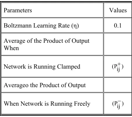
TABLE 3. Parameters used for Boltzmann Learning.
Parameters Values Boltzmann Learning Rate (η) 0.1
Average of the Product of Output When
Network is Running Clamped (Pij+)
Averageo the Product of Output
Transition probability of a node can be given as :
N ) i x
1 ( P ] j [ ] i [
trpb = (20)
Here, N is the number of nodes in the network. Using Equation 20 the probability of self transition can be calculated as
[
1−trpb[i][j]]
. We continue to calculate these transition probabilities for all the states in the network until the first thermal equilibrium is achieved. After achieving the first thermal equilibrium at the initial Temperature (T), the temperature is reduced from T = 0.5 to T = 0.41, the same process is repeated until second thermal equilibrium is achieved. We continue this process of achieving thermal equilibrium for T = 0.32, 0.23, 0.14 and 0.05. At T = 0.05, we obtain the stable states. Now we perform the same process of simulation annealing with clamped data, i.e. the network is run with specified initial weights and these weights are updated as per the Boltzmann’s learning rule as:) f ij p c ij p ( T w= η −
Δ (21)
This process keeps updating the weights until they become stable.
We start with following initial weights to train the neural network:
⎥ ⎥ ⎥
⎦ ⎤
⎢ ⎢ ⎢
⎣ ⎡
−
− =
00000 . 0 46000 . 0 48000 . 0
46000 . 0 00000 . 0 47000 . 0
48000 . 0 47000 . 0 00000 . 0 W
Further these weights are updated using Equation 21 to:
⎥ ⎥ ⎥
⎦ ⎤
⎢ ⎢ ⎢
⎣ ⎡
−
− =
00000 . 0 569398 . 370602 .
569398 . 00000 . 0 579398 .
370602 . 579398 . 00000 . 0
and finally converges to:
⎥ ⎥ ⎥
⎦ ⎤
⎢ ⎢ ⎢
⎣ ⎡ =
0.0000000 0.5765980
0.3634020
-0.5765980 0.0000000
0.5865980
0.3634020
-0.5865980 0.0000000
The algorithm steps of the above discussed method
can be given as:
Begin
1. Select a network of n nodes 2. Set T = 0.5
3. Repeat
4. Generate random weights and assign them to the communication links 5. Repeat
6. Repeat
7. Calculate state probabilities until they become constant
8. Anneal the network until T < = 0.05 9. Clamp the network with calculated
weights
10. Repeat
11. Repeat annealing the network
12. Calculate state probabilities until they become constant
13. Until T < = 0.05//Finding Out Stable States
14. Calculate Energy of each component in the network using proposed model
ij w ) j s ( P ) i j P(si 2
1 j s i j wij si 2
1
] state [ E
∑ ∑ − > >< ∑ ∑ <
=
15. Find out the state with maximum probability
16. If it is the same state with minimum energy then
17. Print “it is a stable state”//calculate the modification in Weights using Boltzmann learning law
18. (pijc pfij) T
w= η − Δ
19. If (i=j) then 20. wc[i][j] = 0: 21. Else
22. Wc[i][j] = wc[i][j] + Δw:
23. Until weight becomes constant 24. Until (n=2n)
25. End.
5. RESULTS AND DISCUSSION
on two types of the networks: a network with three nodes and another with five nodes. The probabilities and energies at various thermal equilibriums are given in table number 5.1 and 5.2 (for a 3 node network). For a 5 nodes network we have the values for 32 states.
5.1. Discussion
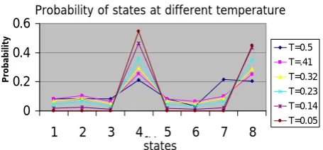
This table represents theprobabilities of different states at various thermal equilibriums. From the values (probabilities of states) in the table we observe that the value of the state which are reliable are increasing as we anneal the network slowly (in our case such states are 011 and 111) where as the value of probability for rest of the states (unreliable) are decreasing to zero. This is the representation that these states cannot be reliable. Figure 1 is the pictorial representation of the Table 4. From this we can observe that in a network of three nodes we have two states (011 and 111) having the highest probabilities and hence are the reliable states among all eight states.
5.1.1. Energy of states at different temperature
Energy landscape throughout the experiments represents the status of stability or instability. When the energy of a network with 3 nodes is calculated using proposed model, we obtain the following values given in Table 5:
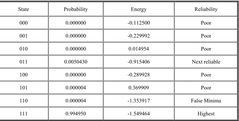
Table 5-8 contains the energy values of the different states in a three node network. From the values of the table we observe that the states 011, 110, and 111 have least energy values. Among these three states we have 011 and 111 as reliable states and 111 as most reliable state as it has global minimum energy. The state 110 has false minima of the energy. From the graph 4.2 we observe that at temperature T = 0.05 the energy of the states
011, 110 and 111 have lowest energy among all other states. These states are assumed to be the reliable states, but from Figure 1 we observe that there are only two reliable states having the maximum probabilities. So states 011 and 111 are the reliable states, out of which only 111 the most reliable state of the network is because it has the lowest energy among all the energy states i.e. the global minimum. Thus, the network will be settled at the 111 for the given condition.
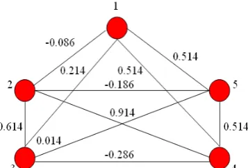
So, the three nodes network architecture will have the most reliable state when all its nodes are in up states and the strength of the links are 0.5865980,-0.3634020 and 0.5765980 between first and second node, second and third node and third and first node respectively as shown in Figure 3.
Let us justify the converged weights those turn the network into a reliable network. At T = 0.05, the energy of the state 111 with these weights is minimum as shown and discussed in Figure 2. As discussed already in Section 4 these weights are obtained from initial weights after processing Boltzman’s learning rule and remains constant.
5.1.2. Comparison of performance with combinatorial approach Let us compare the
results of this approach with the conventional combinatorial approaches for that we consider a network of type hypercube H6 with 26 = 64 nodes
and 25.6 = 192 edges. Following table gives the
performance of the network as follows:
This table depicts that when the probability of being up of the nodes and edges is highest then the reliability of the network is also highest. Our proposed algorithm is employing the neural network optimization approach, which gives an alternate method for calculating the network reliability of the network. In our method we have a certainty of having at least one state as most reliable state. In the network of three nodes we have obtained such reliable state in which all nodes are in up states and the weights are adjusted accordingly to make it most reliable state.
In the network of five nodes we have obtained such reliable state in which all nodes are in up states and the weights are adjusted accordingly to make it most reliable state.
5.2. Discussion
From the Figure 4 we can observeProbability of states at different temperature
0 0.2 0.4 0.6
1 2 3 4St t 5 6 7 8
P
roba
bi
li
ty T=0.5
T=.41 T=0.32 T=0.23 T=0.14 T=0.05
states
Figure 1.Probabilitiesof states at different temperature(for a 3 node network).
Probabilit
TABLE 4. Stationary Probabilities Distribution of States at Different Temperatures.
T = 0.5 0.084 0.0839 0.0839 0.211 0.0839 0.0321 0.215 0.206
T = 0.41 0.0835 0.103 0.0641 0.255 0.0828 0.0631 0.102 0.25
T = 0.32 0.0692 0.088 0.0504 0.293 0.0687 0.0496 0.0871 0.286
T = 0.23 0.0485 0.0642 0.0328 0.361 0.0478 0.0319 0.063 0.348
T = 0.14 0.0172 0.0237 0.0108 0.465 0.0169 0.0102 0.0231 0.434
T = 0.05 0.000051 0.000073 0.000032 0.547 0.000049 0.000028 0.000068 0.448
TABLE 5. Stationary Probabilities Distribution of States at Different Temperatures.
T = 0.5 -0.1125 -0.19706 -0.08664 -0.69185 -0.2887 0.370602 -1.35759 -1.55638
T = 0.41 -0.1125 -0.20862 -0.07706 -0.71804 -0.31205 0.090236 -1.05543 -1.310019
T = 0.32 -0.1125 -0.21136 -0.06159 -0.75639 -0.32231 0.128726 -1.01249 -1.35469
T = 0.23 -0.1125 -0.22179 0.036342 -0.81256 -0.32481 0.19432 -1.20874 -1.40249
T = 0.14 -0.1125 -0.2284 -0.00168 -0.88277 -0.30786 0.305403 -1.30469 -1.047231
T = 0.05 -0.1125 -0.22999 0.014954 -0.91541 -0.28993 0.369909 -1.35392 -1.549469
TABLE 6. Reliabilty of Network at a Specified Node and Edge Probability.
Pv 0.7 0.8 0.9 0.95 0.95 0.95 0.95 0.99
Pe 0.7 0.8 0.9 0.95 0.96 0.97 0.98 0.99
that in a network of five nodes the probabilities of different states at different temperatures. The probabilities of most of the states are close to zero, which represents the unreliable states of the network. But at T = 0.05 the states 11100, 10100 and 11111 have maximum probabilities and hence may represent reliable states but out of which only 11111 is the most reliable state of the network. Let us discuss the behavior of a five node network. We started with random initial weights. After the learning these weights get converged as shown into the Figure 5.
A network with 5 nodes may be in any one of the 25 = 32 states. But when the nodes are in up
states and the links have converged weights then at T=0.05, the energy of the state 11111 is minimum. As discussed already in Section 4 these weights are obtained from initial weights after processing Boltzman’s learning rule and remains constant.
6. CONCLUSION
From the above said discussions we can conclude that the network reliability can be estimated using
Neural Optimization tools like Hopfield model, Simulation Annealing and Boltzmann Learning. This new approach of estimating the network reliability provides a wider range of output as compared to the existing models. Our proposed model when compared with the existing model [20] the following similarities and dissimilarities can observe:
1. Both models are developed for a network having unreliable node and communication link, i.e. at any instant of time any component or any link of the network can be failed. 2. The previous model is based on the up and
down probabilities of the different component in the network and our proposed model based on the average value of the output (probability density function) of the different components.
3. We proposed a model based on simulation annealing whereas the previous model of estimating the reliability of a network based upon combinatorial approach.
4. The proposed model specifies the reliability of the network as well as the different reliable states, whereas the previous model gives only the reliability of the network. TABLE 7. Reliability of a Network of three Nodes using Neural Optimization at T = 0.05.
State Probability Energy Reliability
000 0.000000 -0.112500 Poor
001 0.000000 -0.229992 Poor
010 0.000000 0.014954 Poor
011 0.0050430 -0.915406 Next reliable
100 0.000000 -0.289928 Poor
101 0.000004 0.369909 Poor
110 0.000004 -1.353917 False Minima
TABLE 8. Reliability of a Network of Five Nodes using Neural Optimization at T = 0.05.
State Probability Energy Reliability
00000 0.000000 0.000000 Poor
00001 0.000000 -1.000000 Poor
00010 0.000000 -1.000000 Poor
00011 0.000000 -4.200000 Poor
00100 0.000000 -1.000000 Poor
00101 0.000000 -3.700000 Poor
00110 0.000000 -3.400000 Poor
00111 0.000000 -8.300000 False Minima
01000 .000000 -1.000000 Poor
01001 0.000000 -3.500000 Poor
01010 0.000000 -4.600000 Third Reliable
01011 0.000000 -9.496200 False Minima
01100 0.000000 -4.365400 Poor
01101 0.000000 -8.696200 False Minima
01110 0.000000 -9.496200 False Minima
01111 0.000000 -16.092400 False Minima
10000 0.000000 -1.000000 Poor
10001 0.000000 -4.265400 Poor
10010 0.000000 -4.265400 Poor
10011 0.000000 -9.796200 Second Reliable
10100 0.000000 -4.086600 Poor
10101 0.000000 -9.359800 False Minima
10110 0.000000 -9.059800 False Minima
10111 0.000000 -16.719600 False Minima
11000 0.000000 -3.786600 Poor
11001 0.000000 -8.859800 False Minima
11010 0.000000 -9.959800 False minima
11011 0.056666 -17.419600 False Minima
11100 0.000000 -9.359800 False Minima
11101 0.000000 -16.319600 False Minima
11110 0.000196 -17.119600 False Minima
Energy of states at different temperatures
-2 -1.5 -1 -0.5 0 0.5
1 2 3 4 5 6 7 8
States
En
e
rgy
T=0.5 T=0.41 T=0.32 T=0.23 T=0.14 T=0.05
Figure 2. Energy of states at different temperature (for a 3 node network).
Figure 3. Network architecture for the most reliable stable state for three nodes.
Probability of states of a network with 5 nodes
0 0.1 0.2 0.3 0.4 0.5 0.6 0.7
1 3 5 7 9 11 13 15 17 19 21 23 25 27 29 31 33
Pr
o
b
a
b
il
it
y
T=.50
T=.41
T=.32
T=.23
T=.14
T=.05
states
Figure 4. Probabilities of states (for a network with 5 nodes).
5. The main drawback of the combinatorial approach is its complexity, as the size of the network increases the complexity also increases exponentially. But proposed model overcomes this drawback of existing model and reduces the complexity.
We have the following observations for the proposed approach:
1. Minimum energy states represent the reliable states of the network
2. We can obtain more than one global minimum energy states, but out of these states, only one state with lowest energy will be the most reliable state of the network, which ensures successful communication.
3. Rest of the states, with lower energy (or higher probability), are the cases of false energy minima in the network, which can not be avoided.
4. In any case of failure of any component or communication links in the network, the network will settle to the most reliable state (state with least global energy) of the network for successful communication. We have considered a network of three nodes and five nodes, the future work can be extended for a network with more nodes. The researchers may extend this work to calculate the upper bound and the lower bound of the network reliability using neural network as a tool.
7. REFERENCES
1. Hui, K.P.,“Network Reliability Estimation”, Ph.D. Dissertation, Faculty of Engineering, Computer and Mathematical Science, University of Adelaide, Adelaide, Australia, (2005).
2. Boudali, H. and Dugan, J.B., “A Discrete Time Bayesian Network Reliability Modeling and Analysis Frame Work”, Reliability and System Safety, Vol. 3,
No. 87, (2005), 337-349.
3. Lomonosov, M. and Shpungin, Y., “Combinatorics of Reliability Monte Carlo”, Random Structures and Algorithms, Vol. 4, No. 14, (1999), 329-343.
4. Barlow, R. E., “A survey of Network Reliability and Domination Theory”, Operation Research, Vol. 32, (1984), 478-492.
5. Ball, M.O., Complexity of Network Reliability Computation”, Networks, Vol. 10, (1980), 153-165.
6. Barlow, R.E. and Proschan, F., “Statistical Theory of Reliability and Life Testing”, Holt, Rinehart and Winston, Concord, CA , U.S.A., (1975).
7. Colbourn, C.J., “The Combinatorics of Network Reliabilty”, Oxford University Press, New York, U.S.A., (1987). 8. Colbourn, C.J., Satyanarayana, A., Suffel, C. and
Sutner, K., “Computing Residual Connectedness Reliability for Restricted Networks”, Discrete Applied Mathematics, Vol. 44, (1993), 221-232.
9. Lucia, I.P., “Implementation of Factoring Algorithm For Reliability Evaluation of Undirected Networks”, IEEE, Transaction on Reliability, Vol. 37, (1988), 462-468. 10. Easton, M.C. and Wong, C.K., “Sequential Destruction
Method for Monte Carlo Evaluation of System Reliability”, IEEE Transaction on Reliability, Vol.
R-29, (1980), 27-32.
11. Elperin, T., Gertsbakh, I. and Lomonosov, M., “Estimation of Network Reliability using Graph Evolution Models”,
IEEE Transactions on Reliability, Vol. 5 No. 40,
(1991), 572-581.
12. Elperin, T., Gertsbakh, I. and Lomonosov, M., “An Evolution Model for Monte Carlo Estimation of Equilibrium Network Renewal Parameters”, Probability
in the Engineering and Informational Sciences, Vol.
6, (1992), 457-469.
13. Fishman, G.S., “A Monte Carlo Sampling Plan for Estimating Network Reliability”, Operations Research,
Vol. 34, (1986), 581-592.
14. Fishman, G.S., “A Monte Carlo Sampling Plan for Estimating Reliability Parameters and Related Functions”,
Networks, Vol. 17, (1987), (169-186).
15. Hui, K.P., Bean, N., Kraetzl, M. and Kroese, D.P., “The Tree Cut and Merge Algorithm for Estimation of Network Reliability”, Probability in the Engineering and Informational Sciences, Vol. 1, 17, (2003), 24-25. 16. Kumamoto, H., Kazuo, T., Koichi, I. and Henley, E.J.,
“State Transition Monte Carlo for Evaluating Large, Repairable Systems”, IEEE Trans. Reliability, Vol.
R-29, (1980), 376-380.
17. Lomonosov, M., “On Monte Carlo Estimates in Network Reliability”, Probability in the Engineering and Information Sciences, Vol. 8, (1994), 245-264.
18. Shpungin, Y., “Combinatorial and Computational Aspects of Monte Carlo Estimation of Network Reliability”, PhD. Dissertation, Dept. of Mathematics and Computer Science, Ben Gurion University of the Negev, New York, U.S.A., (1996).
19. Gertsbakh, and Shpungin, Y., “Combinatorial Approaches to Monte Carlo Estimation of Network Lifetime Distribution”, Appl. Stochastic Models Bus. Ind., Vol. 20, (2004), 49-57.
20. Shpungin, Y., “Combinatorial Approach to Reliability Evaluation of Network with Unreliable Nodes and Unreliable Edges”, International Journal of Computer Science, Vol. 3, No. 1, (2006), 177-182.
21. Yegnanrayana, B., “Artificial Neural Network”, Ed. 2, Prentice-Hall of India (P) Ltd., New Delhi, India, (1999), 149-196.
617-621.
23. Hertz, J.A., Krogh, A. and Palmer, R.G., “Introduction to the Theory of Neural Computation”, Addission-Wesley, New York, U.S.A., (1991).
24. Muller, B. and Reinhard, J., “Neural Networks: An Introduction, Physics of Neural Networks”, Springer-Verlag, New York, U.S.A., (1991).
25. Ratana, C.S. and Smith, A.E., “Estimating All Terminal Network Reliability Using Neural Network”, Computer and Operation Research, Vol. 29, No. 7, (2002), 849-868.
26. Hopfield, J.J. and Tank, D.W., “Neural Computation of
Decisions in Optimization Problems”, Biological Cybernetics, Vol. 52, No. 3 (1985), 141-152.
27. Yuille, A.L., “Constrained Optimization and the Elastic Net”, In the Hand Book of Brain Theory and Neural Networks, Cambridge, MA: MIT Press, U.S.A., (1995), 250-255.
28. Kirkpatrick, S., Gelatt, C.D. and Vecchi, M.P., “Optimization by Simulated Annealing”, Science, Vol.
220, (1983), 671-680.