Please cite this article as: M. Gorji, H. Ghassemi, J. Mohammadi, Determining the Hydro-Acoustic Characteristics of the Ship Propeller in Uniform and Non-uniform Flow, International Journal of Engineering (IJE), TRANSACTIONS A: Basics Vol. 29, No. 4, (April 2016) 530-538
International Journal of Engineering
J o u r n a l H o m e p a g e : w w w . i j e . i rDetermining the Hydro-acoustic Characteristics of the Ship Propeller in Uniform and
Non-uniform Flow
M. Gorjia, H. Ghassemi*b, J. Mohammadia
a Department of Marine Engineering, MalekAshtar University of Technology, Shahinshahr, Iran
b Department of Marine Engineering, Amirkabir University of Technology, Tehran, Iran
P A P E R I N F O
Paper history:
Received 27 February 2016
Received in revised form 14 April 2016 Accepted 14 April 2016
Keywords:
Marine Propeller Sound Pressure Level Hydrodynamic Performance Noise Reduction
A B S T R A C T
This research has been carried out to determine the marine propeller hydro-acoustic characteristics by Reynolds-Averaged Navier-Stokes (RANS) solver in both uniform and non-uniform wake flow at different operating conditions Wake flow can cause changes in pressure fluctuation and gas effect on propeller noise spectrum. Noise is generated by the induced trailing vortex wake and induced pressure pulses. The two-step Fflowcs Williams and Hawkings (FW-H) equations are used to calculate hydrodynamic pressure and its performance as well as sound pressure level (SPL) at various points around the propeller. The directivity patterns of this propeller and accurate explanation of component propeller noise are discussed. Comparison of the numerical results shows good agreement with the experimental data.Based on these results, effects of wake flow and operating conditions on the noise reduction are investigated.
doi: 10.5829/idosi.ije.2016.29.04a.12
NOMENCLATURE
Cp Pressure coefficient
D Diameter
g Gravity acceleration
J Advance velocity ratio
k Wave number
Kt Trust coefficient
Kq Torque coefficient
n RPM
p Pressure
r Radius
t Time
u Velocity
Efficiency
Density
Shear stress
*
1. INTRODUCTION
Various factors, including environmental and structural factors play an important role in the generation of underwater noise. Ship’s propeller creates noise from its working behind the ship to make the thrust for overcoming the resistance at designed speed. Noise generated by the propellers in terms of intensity and spectral has been a strategic issue for warships and military designers over the years. The generated sound can be heard for hundreds of meters below the surface and may be detected by the sonar. In design process, specifically for marine propellers, it should be tried to reach lowest noise possible [1]. Generally, there are two main sources of noise; one due to mechanical elements like engine, and the second one by hydrodynamic source i.e. by the propeller [2]. Research is needed on the noise sources in order to reduce the noise and increase performance quality by making minimal changes in the vessels elements.
Propeller noise usually includes a series of periodic parts or tones at blade rate and its multiples. These periodic unsteady forces impose discrete tonal noise at the blade passing frequency (BPF). Together with a broadband noise spectrum caused by turbulence interaction with blade and vortex shedding at the trailing edge and the tips. A small-scale part of turbulent eddies in the wake cause unsteady blade forces. Besides, the boundary layer separation and blades vortex shedding also causes fluctuating forces. Shedding vortex will happen at the area of trailing edge and tip of rotating blades. Induced pressure pulses by the propeller may be considered as one of the important sources in the SPL. Moreover, whereas the propeller operates in the heavy-load condition, the boundary layer around the blade may separate at the stagnation point in the suction side. The flow separation and vortex shedding are completely unsteady events which will impose oscillating pressure on the propeller. So, the underwater propeller will produce noise, even in uniform inflow [3].
Conventional procedures to study the propeller unsteady force are the lifting surface and the panel methods. Kerwin et al. [4] applied the unsteady vortex lattice technique to formulate the unsteady propeller. Hoshino et al. [5] employed the panel method to simulate unsteady flow on propeller. These methods do not for account viscous effects such as the boundary layer and separation flow, and usually repair results with empirical treatments. To conquest the deficiency of potential methods, RANS model have been successfully employed for marine propellers. Funeno et al. [6] studied unsteady flow around a high-skewed propeller in non-uniform inflow. Hu et al. [7] applied RANS model to simulate the test case, DTMB 4119 propeller worked on non-uniform inflow conditions. Li et al. [8] introduced numerical prediction of flow around a
propeller. Numerical simulation of tonal and broadband hydrodynamic noises of none-cavitating underwater propeller has been carried out by Kheradmand et al. [9]. Jang et al. [10] analyzed BPF noise of a propeller comprising of the thickness and loading noises on non-cavitating marine propeller. Wake flow effects on cavitation was investigated by Jafary et al. [11]. Bagery et al. [12] established acoustic Analogy on marine propeller on cavitating and non-cavitating conditions by both experimental and numerical calculations. Analytic source model of propeller non-cavitating noise described by longitudinal quadrupoles and dipoles, was done by Kim et al. [13]. Pan et al. [14] conducted a numerical study on the acoustic radiation of a propeller interacting with non-uniform inflow. Approach for identification of low-frequency noise generation mechanisms in the propeller flow [15] which is due to the cavitating flow is discussed [11].
Some parameters like wake flow and operating conditions may cause hydrodynamic and acoustic changes in propeller characteristics. To the best of our knowledge, there is no study on wake flow effects on propeller noise reduction. The objective of the current study is to conduct a numerical simulation of the acoustic pressure generated by a marine propeller in different wake flow and operating conditions. The far-field radiation is predicted by integral formula FW-H equation, with the solution of the RANS solver. The hydro- acoustic performances of propeller are compared with experimental studies. Acoustic analogy and effect of inflow quality have been done in the last section.
2. WIDE RANGE OF FREQUENCY OF THE PROPELLER NOISE
A wide range of frequencies (low and high frequency) exist in propeller noise as described below. Propeller noise can be classified into three categories: harmonic, broadband, and narrow-band random noise.
Harmonic noise is the periodic component, which can be represented by a pulse which repeats at a constant rate. Broadband noise is random in nature and contains components at all frequencies. Narrow-band random noise is almost periodic. However, examination of the harmonics reveals that the energy is not concentrated at isolated frequencies, but rather it is spread out. The mechanisms which lead to the generation of the spectral characteristics discussed above are described in four categories; Steady Sources, Unsteady Sources, Random Sources and Non Linear Effects [16].
Thickness noise arises from the transverse periodic displacement of the water by the volume of a passing blade element. The amplitude of this noise component is proportional to the blade volume, with frequency characteristics dependent on the shape of the cross section of blade and rotational speed. Thickness noise can be represented by a monopole source distribution and becomes important at high speeds. Thin blade sections and plain form sweep are used to control this noise [1].
Loading noise is a combination of thrust and torque (or lift and drag) components which result from the pressure field that surrounds each blade as a consequence of its motion. This pressure disturbance moving in the medium propagates as noise. Loading source can be represented by a dipole source and becomes an important mechanism at low to moderate speeds.
For moderate blade section speed, the thickness and loading sources are linear and act on the blade surfaces. For high speed propeller, nonlinear effects can become significant. In hydro acoustic theory, these sources can be modeled with quadrupole sources distributed in the volume surrounding the blades. In principle, the quadrupole could be used to account for all the viscous and propagation effects not covered by the thickness and loading sources. In the high speed blade sections, the quadrupole sources is much greater than thickness and loading sources and cause the increase ofthe noise level.
Unsteady sources are time dependent in the rotating-blade frame of reference. They include periodic and random variation of loading on the blades. For example, for a propeller behind an aft wake regardless of the number of blades on the propeller, the loading on the blade varies during a revolution. Unsteady loading is an important source in the counter-rotating propeller.
Unsteady Random sources give rise to broadband noise. For propellers, there are two sources which may be important depending on the propeller design and operating conditions. The first broadband noise source is the interaction of inflow turbulence with the blade leading edges. Since the inflow is turbulent, the resulting noise is random. The importance of this noise source depends on the magnitude of the inflow turbulence, but it can be quite significant under conditions of high turbulence at low speeds.
In the second broadband mechanism, noise is generated near the blade trailing edge. A typical propeller develops a turbulent boundary layer over the blade surfaces which can result in fluctuating blade loading at the trailing edge. The noise is characterized by the boundary layer properties. A related mechanism occurs at the blade tips, where turbulence in the core of the tip vortex interacts with the trailing edge. It has been determined for full-scale propellers that the broadband
noise sources are relatively unimportant and do not contribute significantly to the total noise.
3. ACOUSTIC METHOD BASED ON THE FW-H EQUATION
The first and most accomplished research in aeroacoustic waves has been done by Lightill in 1952 [17]. Two basic governing equations of the continuity and momentum are employed to obtain overall sound production relationship. By writing the continuity equation as follows:
q x u t u div Dt D i i ( ) ( ) . (1)
where q is the mass production rate per unit volume. The momentum equation is expressed as
i i i i j i i f x g x p x u u t u ( ) ( )
. (2)
where fi represents the body forces. From Equation (1) and (2), the Equation (3) is retrieved by following form:
j i ij x x T c t
2( )
2 2 0 2 2
. (3)
Here, C0 is the sound speed and Tij is the Lighthill stress tensor. It is expressed as
ij ij
j i
ij uu p c
T ( 2)
0 . (4)
First term of RHS of the Equation (4) is the turbulence velocity fluctuations (Reynolds stresses), the second term is due to changes in pressure and density and the third term is due to the shear stress tensor.
A generalization of Lighthill’s theory is to include hydrodynamic surfaces in motion. It is suggested by FW-H that has prepared the basis for an important amount of analysis of the noise caused by rotating blades, including propeller and fans. FW-H theory contains surface source terms in addition to the quadruple source. The surface sources are generally indicated thickness (or monopole) sources and loading (or dipole) sources. This equation is presented as follows [18].
(5)
(4). Also H(f) and δ(f) are Heaviside and Dirac delta functions, respectively. By solving this equation, pressure variation and SPL (measured in dB) are calculated by Equation (6) as follows:
. (6)
where prms is the root mean square sound pressure and pref is the reference sound pressure, both measured in Pa.
4. NUMERICAL RESULTS AND DISCUSSIONS
The propeller noise is calculated for comparison with the experimental results. The experimental data was obtained out by Atlar et al. [18]. Main dimensions of the propeller are presented in Table 1. Incompressible finite volume method in commercial ANSYS Fluent 14.5 software is used [19].
An unstructured hybrid mesh was applied for grid generation. Triangular cells are used for Blades and hub surfaces. A fine grid was used for near wall to capture the flow in this region. The grid aspect ratio is gradually increasing to decrease solution costs. A moving reference frame (MRF) was used to generate rotational speed around propeller. The generated grid is shown in Figure 1.
Computational domain is defined at 5D for upstream, 15D at downstream and 10D for side one (D is propeller diameter). About two million cells have been created for whole domain grid, as demonstrated in Figure 2. In order to study the propeller performance in uniform flow and applying open water condition, a rectangular control volume was considered around propeller with velocity inlet and pressure outlet boundary conditions. The domain distances were considered sufficiently large to keep away from blockage effects on the propeller hydrodynamic performance characteristics.
The SIMPLE algorithm is used for pressure-velocity coupling equation and second order upstream discretization for momentum equations. Realizable k-ε model is used to model turbulence with time step equal to 1e-4.
Figure 1. The generated unstructured grid on propeller
Figure 2. The generated unstructured grid on propeller
Figure 3. Coordinate system of the propeller
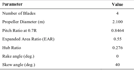
TABLE 1.Main dimensions of the propeller
Parameter Value
Number of Blades 4
Propeller Diameter (m) 2.100
Pitch Ratio at 0.7R 0.8464
Expanded Area Ratio (EAR) 0.55
Hub Ratio 0.276
Rake angle (deg.) 0
Skew angle (deg.) 40
To capture sound, the receivers are adjusted in four points above the propeller at z-axis (z/D=0.5, 1, 1.5, 2) and also at four points downstream locations (x/D=0.5, 1, 1.5, 2) from center of the propeller as shown in the coordinate system of the propeller in Figure 3. Figure 4 shows the wake distribution which displayed excellent wake uniformity due to the stern form.
are shown in Figures 7 and 8 at four radial sections (r/R=0.3, 0.5, 0.7, 0.9) on the blade.
-1 0 1 2
r/R -1.5 -1 -0.5 0 0.5 1 1.5 r/ R
0.500
0
.500
0.6 00 0.6 0 0 0 .700
0.7 0 0
0.80
0
0.8 00
0.900
0
10 20 30 40 50 60 70 80 90 100 110 120 130 140 15 0 1 6 0 1 7 0 1 8 0 19 0 20 0 21 0 220 230 240 250 260 270 280 290 300 310 320 3 30 3 4 0 3 5 0
NON-DIMENSIONAL AXIAL VELOCITY DISTRIBUTION
0
10 20 30 40 50 60 70 80 90 100 110 120 130 140 15 0 1 6 0 1 7 0 1 8 0 19 0 20 0 21 0 220 230 240 250 260 270 280 290 300 310 320 3 30 3 4 0 3 5 0
NON-DIMENSIONAL AXIAL VELOCITY DISTRIBUTION
V/Vs 1.000 0.900 0.800 0.700 0.600 0.500
Figure 4. Non-uniform wake flow field [20]
(a)
(b)
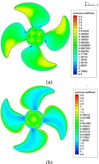
Figure 5. Pressure coefficient distribution on normal load condition (J=0.74) (a) pressure side (b) suction side
(a)
(b)
Figure 6. Pressure coefficient distribution on heavy load condition (J=0.29) (a) pressure side (b)suction side
Figure 7. Pressure coefficient distribution on blade section for normal load condition (J=0.74)
Figure 8. Pressure coefficient distribution on blade section for heavy load condition (J=0.29)
around propeller in Figure 10. Figure 11 illustrates two views of distribution axial velocity, where propeller is rotating with a constant rotational velocity of 197 rpm.
As seen in this figure, blade tip produces high speed backward flow (regions marked red). At the same time a forward flow with lower axial velocity is also generated. These two reverse flows stimulate a vertical flow around the blade tip.
Figure 9. Hydrodynamic characteristics of the propeller
(a)
(b)
Figure 10. Pressure coefficient distribution for normal (a) and heavy load (b) condition in propeller downstream
(a) (b)
(c) (d)
Figure 11. Axial velocity distribution in blade section and downstream for normal load condition (a, b) and heavy load condition (c, d)
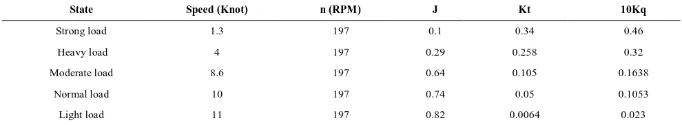
TABLE 2. Hydrodynamic characteristics results at five operating conditions
State Speed (Knot) n (RPM) J Kt 10Kq
Strong load 1.3 197 0.1 0.34 0.46
Heavy load 4 197 0.29 0.258 0.32
Moderate load 8.6 197 0.64 0.105 0.1638
Normal load 10 197 0.74 0.05 0.1053
5. SPL AROUND PROPELLER
In the following section, the flow field around rotating blades, is described in detail. The noise source strength was achieved and acoustic analogy approximation can be used to assess the numerical broadband noise.
The density and sound speed in water are 1000 kg/m3 and 1480 m/s. The reference pressure for SPL is 1.0 μPa.
Numerical calculations of the SPL and experimental data are shown in Figure 12 at z/D=1.5 for normal load condition. There is a good agreement between the numerical and experimental results. As seen from diagram, the peak noise level (143 dB) occurrs at frequency around 80(Hz). For frequencies between 1,000~3000 the SPL is dropped to 100dB.
Noise spectrum for other receivers at above the propeller (z/D = 0.5, 1, 1.5, 2) is shown in Figure 13 for normal load in non-uniform flow. As shown, the overall SPL decreases as the distance from the sound source increases. In the far field, where sound propagates as spherical waves and kr >> 1(k is the wave number and r is the distance to sound source), sound pressure follows the inverse square law with respect to the distance. This means that, in the far-field, the overall SPL is proportional to reverse square of the distance. For instance, if the distance doubles, the overall SPL reduces around 6 to 7 dB. As discussed, this comment uses to predict the proper magnitude just for the far-field. As shown in this figure, SPL for z/D=0.5 and z/D= 1 is varied about 12 dB. For further distances, when the distance doubled, SPL varies about 7 dB.
The noise spectrum is shown in Figure 14 at downstream positions (x/D = 0.5, 1, 1.5, 2). For high frequency, a different procedure is observed. Vortex shedding effect and downstream flow cause different path and sound pressure is reduced slowly. But, in low frequency reverse relation with distance is observed.
Figure 12. SPL spectrum extract from experimental and numerical results in frequency domain at normal load condition and z/D=1.5
5. 1. Operation Condition and Wake Effects on
Noise Reduction The SPL has been figured to be
fairy complex due to complicated physics of viscous influence and vortex manner in the flow above propeller blades. The sound is produced by the Lighthill tensor, the oscillating force and torque, which are seriously influenced by turbulence and nonlinear interactions in vortex flow.
Figure 13. SPL spectrum extract from numerical results in frequency domain for receiver in 4 positions z/D=0.5, 1, 1.5, 2 for normal load condition
Figure 14. SPL spectrum extract from numerical results in frequency domain for receiver in 4 positions x/D=0.5, 1, 1.5, 2 for normal load condition
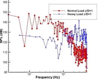
SPL diagram are displayed in Figures 15 at heavy and normal load conditions for z/D=1. In order to have equal rotational speed, as stated above the operation conditions, thickness noise is equal in both but the differences in SPL arise from harmonic noise, loading noise and broadband trailing edge noise that are monopole, dipole and quadrupole, respectively. As will be discussed later, for low speed propeller, nonlinear effects can become insignificant. As seen from this figure, noise level in normal load condition is stronger than heavy load condition in low frequency because of strong Harmonic noise. The tonal peaks at multiples of the BPF are clearly observed on the spectrum plat. On the other hand, the noise for heavy load condition is stronger than normal load condition in high frequency because of strong pressure field (Figures 3 and 4) and loading noise.
SPL chart is illustrated in Figure 16 for x/D=2 in both conditions. Noise level for normal load condition is stronger than heavy load in this position for both low and high frequencies. Strong dipole loading noise can cause strong SPL.
The comparison between Noise spectrum uniform and non-uniform flow is illustrated in Figures 17 and 18 for x/D=1.5 and z/D=1.5. The Result show that SPL increase about 10 percent in wake flow (non-uniform flow) in both low and high frequency.
Figure 16. SPL spectrum extract from numerical results in frequency domain for receiver in x/D=2 for Heavy and normal load conditions
Figure 17. SPL spectrum extract from numerical results in frequency domain for receiver in x/D=1.5 for Uniform and Non-uniform flow
Figure 18. SPL spectrum extract from numerical results in frequency domain for receiver in z/D=1.5 for Uniform and Non-uniform flow
6.CONCLUSION
In order to estimate the wake effect and operation condition on propeller noise, various investigations have been done in this paper. Pressure distribution and hydrodynamic characteristics of the propeller are determined at various operating conditions. Results show good agreement with the experimental results. Varying quality of inlet flow has effect on pressure oscillation and hydrodynamic performance as well as SPL diagram. By inserting wake inflow, sound strength increases about 10 percent. The noise level in different operation conditions is discussed. Based on the results, loading and harmonic sources effect on sound level in different operational condition.
7.REFERENCES
1. Carlton, J., "Marine propellers and propulsion, Butterworth-Heinemann, (2011), 51-60.
2. Crocker, M. J., "Encyclopedia of acoustics", John Wiley, (1997), 94-103.
3. Pan, Y.-c. and Zhang, H.-x., "Numerical hydro-acoustic prediction of marine propeller noise", Journal of Shanghai Jiaotong University (Science), Vol. 15, (2010), 707-712. 4. Kerwin, J. E. and Lee, C.-S., "Prediction of steady and unsteady
marine propeller performance by numerical lifting-surface theory", Society of Naval Architects and Marine Engineers Transactions, Vol. 86, (1978), 218-253.
5. Hoshino, T., "Hydrodynamic analysis of propellers in unsteady flow using a surface panel method", Journal of the Society of Naval Architects of Japan, Vol. 1993, No. 174, (1993), 71-87. 6. Funeno, I., "Analysis of unsteady viscous flows around a highly
skewed propeller", Journal of Kansai Society of Naval Architects, Vol. 237, (2002), 39-45.
7. hu, X.-f., Huang, Z.-y. and Hong, F.-w., "Unsteady hydrodynamics forces of propeller predicted with viscous CFD",
Journal of Hydrodynamics (Ser. A), Vol. 6, (2009), 734-739. 8. Li, W. and Yang, C., "Numerical simulation of flow around a
Polar Engineering Conference, International Society of Offshore and Polar Engineers, (2009).
9. Mousavi, B., Rahrovi, A. and Kheradmand, S., "Numerical simulation of tonal and broadband hydrodynamic noises of non-cavitating underwater propeller", Polish Maritime Research, Vol. 21, No. 3, (2014), 46-53.
10. Jang, J.-S., Kim, H.-T. and Joo, W.-H., "Numerical study on non-cavitating noise of marine propeller", in INTER-NOISE and NOISE-CON Congress and Conference Proceedings, Institute of Noise Control Engineering. Vol. 249, (2014), 3017-3022. 11. Gavzan, I. J. and Rad, M., "Influence of afterbody and boundary
layer on cavitating flow", International Journal of Engineering-Transactions B: Applications, Vol. 22, No. 2, (2009), 185-196.
12. Bagheri, M. R., Mehdigholi, H., Seif, M. S. and Yaakob, O., "An experimental and numerical prediction of marine propeller noise under cavitating and non-cavitating conditions",
Brodogradnja, Vol. 66, No. 2, (2015), 29-45.
13. Kim, D., Lee, K. and Seong, W., "Non-cavitating propeller noise modeling and inversion", Journal of Sound and Vibration, Vol. 333, No. 24, (2014), 6424-6437.
14. Pan, Y.-c. and Zhang, H.-x., "Numerical prediction of marine propeller noise in non-uniform inflow", China Ocean Engineering, Vol. 27, (2013), 33-42.
15. Lidtke, A. K., Humphrey, V. F. and Turnock, S. R., "Feasibility study into a computational approach for marine propeller noise and cavitation modelling", Ocean Engineering, (2015), 33-42. 16. Caridi, D., "Industrial cfd simulation of aerodynamic noise",
Universita degli Studi di Napoli Federico II, (2008),185-196.
17. Lighthill, M. J., "On sound generated aerodynamically. I. General theory", in Proceedings of the Royal Society of London A: Mathematical, Physical and Engineering Sciences, The Royal Society. Vol. 211, (1952), 564-587.
18. Williams, J. F. and Hawkings, D. L., "Sound generation by turbulence and surfaces in arbitrary motion", Philosophical Transactions of the Royal Society of London A: Mathematical, Physical and Engineering Sciences, Vol. 264, No. 1151, (1969), 321-342.
19. CFX, C., "Solver theory, cfx-program (version 11.0) theory documentation", ANSYS Inc., Canonsburg, USA, (2012), 153-161.
20. Atlar, M., Takinaci, A. C., Korkut, E., Sasaki, N. and Aono, T., "Cavitation tunnel tests for propeller noise of a FRV and comparisons with full-scale measurements", caltech. edu/cav2001: sessionB8. 007, (2001), 173-181.
Determining the Hydro-acoustic Characteristics of the Ship Propeller in Uniform and
Non-uniform Flow
M. Gorjia, H. Ghassemib, J. Mohammadia
a Department of Marine Engineering, MalekAshtar University of Technology, Shahinshahr, Iran
b Department of Marine Engineering, Amirkabir University of Technology, Tehran, Iran
P A P E R I N F O
Paper history:
Received 27 February 2016
Received in revised form 14 April 2016 Accepted 14 April 2016
Keywords:
Marine Propeller Sound Pressure Level Hydrodynamic Performance Noise Reduction
ذيكچ ٌ
ٌذض ماجوا صَيژپ سکًتسا زیياو طسًتم سذلًىیر شير ٍب ییایرد یاَ ٍوايزپ یكيماىیديرذيَ شیًو تايصًصخ ٍلاقم هیا رد
RANS رد ي تخاًىكیزيغ ي تخاًىكی نایزج ي .تسا ٌذض یسرزب فلتخم یدزكلمع طیازض رد
یم نایزج کی یير ذواًت
ناذيم تاواسًو .تسا ٌذض یسرزب زتمک شیًو یير زتماراپ هیا زيثات فلتخم یاَ ٍلاقم رد .دراذگب زيثات ٍوايزپ فازطا راطف
شیًو رد
یم داجیا یراطف یاَ سلاپ ي رازف ٍبل سكتري اقلا سا تلاح هیا اَ شمايلیي یا ٍلحزم يد تلاداعم سا .دًض
شگىيکي FW-H یازب
تسا شیًو حطس ي یراطف تاواسًو ٍبساحم تسا ٌذض ٌداف
. ٍب ٍوايزپ شیًو رد زثًم فلتخم یاَزتماراپ ي ٍوايزپ فازطا نایزج ناذيم
ٍک ٌذض ٌدافتسا یبزجت جیاتو سا یكيتسًکا يرذيَ ي یكيماىیديرذيَ جیاتو یجىس رابتعا یازب .تسا ٌذض یسرزب ٍلاقم هیا رد ليصفت
یم ٌذَاطم یبًخ قباطت ٍلاقم هیا سا لصاح جیاتو ساسا زب .دًض
یير زب یيزطيپ تعزس تبسو تازيثات ي یديري کیي تازيثات ،
تسذب ییایرد یاَ ٍوايزپ شیًو حطس آ