Chapter2_An-Itroduction-to-generalized-linear-models.pdf

2

Model Fitting

2.1 Introduction

The model fitting process described in this book involves four steps:

1. Model specification – a model is specified in two parts: an equation linking the response and explanatory variables and the probability distribution of the response variable.

2. Estimation of the parameters of the model.

3. Checking the adequacy of the model – how well it fits or summarizes the data.

4. Inference – calculating confidence intervals and testing hypotheses about the parameters in the model and interpreting the results.

In this chapter these steps are first illustrated using two small examples. Then some general principles are discussed. Finally there are sections about notation and coding of explanatory variables which are needed in subsequent chapters.

2.2 Examples

2.2.1 Chronic medical conditions

Data from the Australian Longitudinal Study on Women’s Health (Brown et al., 1996) show that women who live in country areas tend to have fewer consultations with general practitioners (family physicians) than women who live near a wider range of health services. It is not clear whether this is because they are healthier or because structural factors, such as shortage of doctors, higher costs of visits and longer distances to travel, act as barriers to the use of general practitioner (GP) services. Table 2.1shows the numbers of chronic medical conditions (for example, high blood pressure or arthritis) reported by samples of women living in large country towns (town group) or in more rural areas (country group) in New South Wales, Australia. All the women were aged 70-75 years, had the same socio-economic status and had three or fewer GP visits during 1996. The question of interest is: do women who have similar levels of use of GP services in the two groups have the same need as indicated by their number of chronic medical conditions?

Table 2.1 Numbers of chronic medical conditions of 26 town women and 23 country women with similar use of general practitioner services.

Town

0 1 1 0 2 3 0 1 1 1 1 2 0 1 3 0 1 2

1 3 3 4 1 3 2 0

n = 26, mean = 1.423, standard deviation = 1.172, variance = 1.374

Country

2 0 3 0 0 1 1 1 1 0 0 2 2 0 1 2 0 0

1 1 1 0 2

n = 23, mean = 0.913, standard deviation = 0.900, variance = 0.810

Suppose theY_jk’s are all independent and have the Poisson distribution with parameter θ_j representing the expected number of conditions.

The question of interest can be formulated as a test of the null hypothesis H₀ : θ₁= θ₂ =θ against the alternative hypothesis H₁ :θ₁ =θ₂.The model fitting approach to testing H₀ is to fit two models, one assuming H₀ is true, that is

E(Y_jk) =θ; Y_jk ∼P oisson(θ) (2.1)

and the other assuming it is not, so that

E(Y_jk) =θ_j; Y_jk ∼P oisson(θ_j), (2.2)

wherej= 1 or 2. Testing H₀ against H₁ involves comparing how well models (2.1) and (2.2) fit the data. If they are about equally good then there is little reason for rejecting H₀.However if model (2.2) is clearly better, then H₀would be rejected in favor of H₁.

If H₀ is true, then the log-likelihood function of theY_jk’s is

l₀=l(θ;y) =

J

j=1 Kj

k=1

(y_jklogθ−θ−logy_jk!), (2.3)

where J = 2 in this case. The maximum likelihood estimate, which can be obtained as shown in the example in Section 1.6.2, is

θ= y_jk/N,

whereN =_jK_j. For these data the estimate isθ= 1.184 and the maximum

If H₁is true, then the log-likelihood function is

l₁ = l(θ₁, θ₂;y) =

K1

k=1

(y_1klogθ₁−θ₁−logy_1k!)

+

K2

k=1

(y_2klogθ₂−θ₂−logy_2k!). (2.4)

(The subscripts on l₀ and l₁ in (2.3) and (2.4) are used to emphasize the connections with the hypotheses H₀ and H₁, respectively). From (2.4) the maximum likelihood estimates areθ_j =_ky_jk/K_jforj = 1 or 2. In this case

θ₁= 1.423,θ₂= 0.913 and the maximum value of the log-likelihood function, obtained by substituting these values and the data into (2.4), isl₁=−67.0230. The maximum value of the log-likelihood functionl₁ will always be greater than or equal to that of l₀ because one more parameter has been fitted. To decide whether the difference is statistically significant we need to know the sampling distribution of the log-likelihood function. This is discussed in Chap-ter 4.

If Y ∼ Poisson(θ) then E(Y) = var(Y) = θ. The estimate θ of E(Y) is called the fitted valueofY. The difference Y −θ is called aresidual (other definitions of residuals are also possible, see Section 2.3.4). Residuals form the basis of many methods for examining the adequacy of a model. A residual is usually standardized by dividing by its standard error. For the Poisson distribution an approximate standardized residual is

r= Y−θ θ .

The standardized residuals for models (2.1) and (2.2) are shown in Table 2.2 and Figure 2.1. Examination of individual residuals is useful for assessing certain features of a model such as the appropriateness of the probability distribution used for the responses or the inclusion of specific explanatory variables. For example, the residuals inTable 2.2and Figure 2.1exhibit some skewness, as might be expected for the Poisson distribution.

The residuals can also be aggregated to produce summary statistics measur-ing the overall adequacy of the model. For example, for Poisson data denoted by independent random variables Y_i, provided that the expected valuesθ_iare

not too small, the standardized residuals r_i = (Y_i−θ_i)/

θ_i approximately have the standard Normal distributionN(0,1), although they are not usually independent. An intuitive argument is that, approximately, r_i ∼ N(0,1) so

r2

i ∼χ2(1) and hence

r2 i =

(Y_i−θ_i)2

θ_i ∼χ

2_{(m). (2.5)}

Table 2.2 Observed values and standardized residuals for the data on chronic medical conditions (Table 2.1), with estimates obtained from models (2.1) and (2.2).

Value Frequency Standardized residuals Standardized residuals

of Y from (2.1); from (2.2);

θ= 1.184 θ₁ = 1.423 andθ₂= 0.913

Town

0 6 -1.088 -1.193

1 10 -0.169 -0.355

2 4 0.750 0.484

3 5 1.669 1.322

4 1 2.589 2.160

Country

0 9 -1.088 -0.956

1 8 -0.169 0.091

2 5 0.750 1.138

3 1 1.669 2.184

Residuals for model (2.1)

Residuals for model (2.2)

2 1

0 -1

country town

country town

estimated in order to calculate to fitted values θ_i (for example, see Agresti, 1990, page 479). Expression (2.5) is, in fact, the usual chi-squared goodness of fit statistic for count data which is often written as

X2 ₌(oi−ei)2

e_i ∼χ2(m)

where o_i denotes the observed frequency and e_i denotes the corresponding expected frequency. In this case o_i=Y_i ,e_i=θ_i andr_i2=X2.

For the data on chronic medical conditions, for model (2.1)

r2

i = 6×(−1.088)2+ 10×(−0.169)2+. . .+ 1×1.6692= 46.759.

This value is consistent with r_i2 being an observation from the central chi-squared distribution with m= 23 + 26−1 = 48 degrees of freedom. (Recall from Section 1.4.2, that if X2 ∼χ2(m) then E(X2) =mand notice that the calculated value X2 =r_i2= 46.759 is near the expected value of 48.)

Similarly, for model (2.2)

r2

i = 6×(−1.193)2+. . .+ 1×2.1842= 43.659

which is consistent with the central chi-squared distribution withm= 49−2 = 47 degrees of freedom. The difference between the values ofr_i2from models (2.1) and (2.2) is small: 46.759−43.659 = 3.10. This suggests that model (2.2) with two parameters, may not describe the data much better than the simpler model (2.1). If this is so, then the data provide evidence supporting the null hypothesis H₀:θ₁=θ₂.More formal testing of the hypothesis is discussed in Chapter 4.

The next example illustrates steps of the model fitting process with contin-uous data.

2.2.2 Birthweight and gestational age

The data in Table 2.3 are the birthweights (in grams) and estimated gesta-tional ages (in weeks) of 12 male and female babies born in a certain hospital. The mean ages are almost the same for both sexes but the mean birthweight for boys is higher than the mean birthweight for girls. The data are shown in the scatter plot inFigure 2.2. There is a linear trend of birthweight increasing with gestational age and the girls tend to weigh less than the boys of the same gestational age. The question of interest is whether the rate of increase of birthweight with gestational age is the same for boys and girls.

Let Y_jk be a random variable representing the birthweight of the kth baby in groupjwherej= 1 for boys andj = 2 for girls andk= 1, . . . ,12. Suppose that the Y_jk’s are all independent and are Normally distributed with means

μ_jk = E(Y_jk), which may differ among babies, and variance σ2 which is the same for all of them.

A fairly general model relating birthweight to gestational age is

Table 2.3 Birthweight and gestational age for boys and girls.

Boys Girls

Age Birthweight Age Birthweight

40 2968 40 3317

38 2795 36 2729

40 3163 40 2935

35 2925 38 2754

36 2625 42 3210

37 2847 39 2817

41 3292 40 3126

40 3473 37 2539

37 2628 36 2412

38 3176 38 2991

40 3421 39 2875

38 2975 40 3231

Means 38.33 3024.00 38.75 2911.33

42 40

38 36

34 3500

3000

2500

Gestational age Birth weight

where x_jk is the gestational age of the kth baby in group j. The intercept parameters α₁ and α₂ are likely to differ because, on average, the boys were heavier than the girls. The slope parameters β₁ andβ₂ represent the average increases in birthweight for each additional week of gestational age. The ques-tion of interest can be formulated in terms of testing the null hypothesis H₀:

β₁=β₂ =β (that is, the growth rates are equal and so the lines are parallel), against the alternative hypothesis H₁:β₁=β₂.

We can test H₀ against H₁ by fitting two models

E(Y_jk) =μ_jk =α_j+βx_jk; Y_jk ∼N(μ_jk, σ2), (2.6)

E(Y_jk) =μ_jk =α_j+β_jx_jk; Y_jk ∼N(μ_jk, σ2). (2.7)

The probability density function for Y_jk is

f(y_jk;μ_jk) = √ 1

2πσ2 exp[− 1

2σ2(yjk−μjk)

2_].

We begin by fitting the more general model (2.7). The log-likelihood func-tion is

l₁(α₁, α₂, β₁, β₂;y) =

J

j=1 K

k=1

[−1

2log(2πσ

2₎₋ 1

2σ2(yjk −μjk)

2_]

= −1

2JKlog(2πσ

2₎₋ 1

2σ2

J

j=1 K

k=1

(y_jk−α_j−β_jx_jk)2

where J = 2 and K = 12 in this case. When obtaining maximum likelihood estimates ofα₁, α₂, β₁andβ₂ we treat the parameterσ2 as a known constant, or nuisance parameter, and we do not estimate it.

The maximum likelihood estimates are the solutions of the simultaneous equations

∂l₁ ∂α_j =

1

σ2

k

(y_jk−α_j−β_jx_jk) = 0,

∂l₁ ∂β_j =

1

σ2

k

x_jk(y_jk−α_j−β_jx_jk) = 0, (2.8)

where j = 1 or 2.

An alternative to maximum likelihood estimation is least squares estima-tion. For model (2.7), this involves minimizing the expression

S₁=

J

j=1 K

k=1

(y_jk−μ_jk)2 =

J

j=1 K

k=1

The least squares estimates are the solutions of the equations

∂S₁

∂α_j = −2 K

k=1

(y_jk−α_j−β_jx_jk) = 0,

∂S₁

∂β_j = −2 K

k=1

x_jk(y_jk−α_j−β_jx_jk) = 0. (2.10)

The equations to be solved in (2.8) and (2.10) are the same and so maximizing

l₁ is equivalent to minimizing S₁. For the remainder of this example we will use the least squares approach.

The estimating equations (2.10) can be simplified to

K

k=1

y_{jk −}Kα_j−β_j K

k=1

x_jk = 0,

K

k=1

x_jky_{jk −}Kα_j K

k=1

x_jk−β_j K

k=1 x2

jk = 0

forj = 1 or 2. These are called the normal equations. The solution is

b_j = K

kxjkyjk−(

kxjk)(

kyjk) K_kx2

jk−(

kxjk)2 ,

a_j = y_j−b_jx_j,

wherea_j is the estimate of α_j and b_j is the estimate of β_j,for j= 1 or 2. By considering the second derivatives of (2.9) it can be verified that the solution of equations (2.10) does correspond to the minimum of S₁. The numerical value for the minimum value forS₁ for a particular data set can be obtained by substituting the estimates forα_j and β_j and the data values for y_jk and

x_jk into (2.9).

To test H₀ : β₁ = β₂ = β against the more general alternative hypothesis H₁, the estimation procedure described above for model (2.7) is repeated but with the expression in (2.6) used for μ_jk. In this case there are three parameters, α₁, α₂ and β, instead of four to be estimated. The least squares expression to be minimized is

S₀ =

J j=1 K k=1

(y_jk−α_j−βx_jk)2. (2.11)

From (2.11) the least squares estimates are given by the solution of the simultaneous equations

∂S₀

∂α_j = −2 K

k=1

(y_jk−α_j−βx_jk) = 0,

∂S₀

∂β = −2 J j=1 K k=1

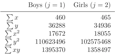
Table 2.4 Summary of data on birthweight and gestational age in Table 2.3 (sum-mation is over k=1,...,K where K=12).

Boys (j= 1) Girls (j= 2)

_x

460 465

_y

36288 34936

_x2

17672 18055

_y2

110623496 102575468

_xy

1395370 1358497

for j = 1 and 2. The solution is

b = K

jkxjkyjk−j(kxjkkyjk) K_jkx2

jk−

j(

kxjk)2 ,

a_j = y_j−bx_j.

These estimates and the minimum value for S₀ can be calculated from the data.

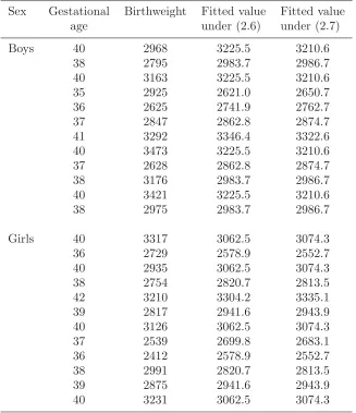
For the example on birthweight and gestational age, the data are summa-rized inTable 2.4 and the least squares estimates and minimum values forS₀ andS₁are given inTable 2.5. The fitted valuesy_jk are shown inTable 2.6. For model (2.6), y_jk =a_j+bx_jk is calculated from the estimates in the top part ofTable 2.5. For model (2.7),y_jk =a_j+b_jx_jk is calculated using estimates in the bottom part of Table 2.5. The residual for each observation isy_jk−y_jk. The standard deviationsof the residuals can be calculated and used to obtain approximate standardized residuals (y_jk−y_jk)/s.Figures 2.3and2.4show for models (2.6) and (2.7), respectively: the standardized residuals plotted against the fitted values; the standardized residuals plotted against gestational age; and Normal probability plots. These types of plots are discussed in Section 2.3.4. The Figures show that:

1. Standardized residuals show no systematic patterns in relation to either the fitted values or the explanatory variable, gestational age.

2. Standardized residuals are approximately Normally distributed (as the points are near the solid lines in the bottom graphs).

3. Very little difference exists between the two models.

The apparent lack of difference between the models can be examined by testing the null hypothesis H₀ (corresponding to model (2.6)) against the alternative hypothesis H₁(corresponding to model (2.7)). If H₀is correct, then the minimum valuesS₁andS₀should be nearly equal. If the data support this hypothesis, we would feel justified in using the simpler model (2.6) to describe the data. On the other hand, if the more general hypothesis H₁ is true then

Table 2.5 Analysis of data on birthweight and gestational age inTable 2.3.

Model Slopes Intercepts Minimum sum of squares

(2.6) b= 120.894 a₁ =−1610.283 S₀= 658770.8

a₂ =−1773.322

(2.7) b₁ = 111.983 a₁ =−1268.672 S₁= 652424.5

b₂ = 130.400 a₂ =−2141.667

Table 2.6 Observed values and fitted values under model (2.6) and model (2.7) for data inTable 2.3.

Sex Gestational Birthweight Fitted value Fitted value

age under (2.6) under (2.7)

Boys 40 2968 3225.5 3210.6

38 2795 2983.7 2986.7

40 3163 3225.5 3210.6

35 2925 2621.0 2650.7

36 2625 2741.9 2762.7

37 2847 2862.8 2874.7

41 3292 3346.4 3322.6

40 3473 3225.5 3210.6

37 2628 2862.8 2874.7

38 3176 2983.7 2986.7

40 3421 3225.5 3210.6

38 2975 2983.7 2986.7

Girls 40 3317 3062.5 3074.3

36 2729 2578.9 2552.7

40 2935 3062.5 3074.3

38 2754 2820.7 2813.5

42 3210 3304.2 3335.1

39 2817 2941.6 2943.9

40 3126 3062.5 3074.3

37 2539 2699.8 2683.1

36 2412 2578.9 2552.7

38 2991 2820.7 2813.5

39 2875 2941.6 2943.9

34 36 38 40 42 -1

0 1 2

Gestational age

R

esidu

als

Model (2.6)

2600 2800 3000 3200 3400 -1

0 1 2

Fitted values

Re

si

du

al

s

Model (2.6)

2 1

0 -1

-2 99

90

50

10

1

Residuals

Per

ce

n

t

Model (2.6)

34 36 38 40 42 -1

0 1 2

Gestational age

Re

si

d

u

al

s

Model (2.7)

2 1

0 -1

-2 99

90

50

10

1

Residuals

Per

ce

n

t

Model (2.7)

2600 2800 3000 3200 3400

-1 0 1 2

Fittted values

Re

si

d

u

al

s

Model (2.7)

sampling distributions of the corresponding random variables

S₁=

J

j=1 K

k=1

(Y_jk−a_j−b_jx_jk)2

and

S₀=

J

j=1 K

k=1

(Y_jk−a_j−bx_jk)2.

It can be shown (see Exercise 2.3) that

S₁ =

J

j=1 K

k=1

[Y_jk−(α_j+β_jx_jk)]2−K

J

j=1

(Y_j−α_j−β_jx_j)2

− J

j=1

(b_j−β_j)2(

K

k=1 x2

jk −Kx2j)

and that the random variables Y_jk, Y_j and b_j are all independent and have the following distributions:

Y_{jk ∼} N(α_j+β_jx_jk, σ2),

Y_{j ∼} N(α_j+β_jx_j, σ2/K),

b_{j ∼} N(β_j, σ2/(

K

k=1 x2

jk−Kx2j)).

ThereforeS₁/σ2 is a linear combination of sums of squares of random vari-ables with Normal distributions. In general, there are JK random variables (Y_jk −α_j −β_jx_jk)2/σ2, J random variables (Y_j −α_j −β_jx_j)2K/σ2 and J random variables (b_j −β_j)2(_kx2_jk −Kx2_j)/σ2. They are all independent and each has the χ2(1) distribution. From the properties of the chi-squared distribution in Section 1.5, it follows that S₁/σ2 ∼ χ2(JK −2J). Similarly, if H₀ is correct then S₀/σ2 ∼ χ2[JK −(J + 1)]. In this example J = 2 so

S₁/σ2 _{∼ χ}2_{(2K −4) and S}

0/σ2 ∼ χ2(2K −3). In each case the value for

the degrees of freedom is the number of observations minus the number of parameters estimated.

If β₁ and β₂ are not equal (corresponding to H₁), then S₀/σ2 will have a non-central chi-squared distribution with JK −(J + 1) degrees of freedom. On the other hand, provided that model (2.7) describes the data well, S₁/σ2 will have a central chi-squared distribution withJK−2J degrees of freedom. The statistic S₀−S₁ represents the improvement in fit of (2.7) compared to (2.6). If H₀ is correct, then

1

σ2(S0−S1)∼χ2(J −1).

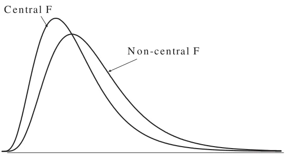
distribu-N o n -c e n tra l F C e n tra l F

Figure 2.5 Central and non-central F distributions.

tion. However, as σ2 is unknown, we cannot compare (S₀−S₁)/σ2 directly with the χ2(J −1) distribution. Instead we eliminate σ2 by using the ratio of (S₀−S₁)/σ2 and the random variable S₁/σ2 with a central chi-squared distribution, each divided by the relevant degrees of freedom,

F = (S0−S1)/σ

2

(J−1) / S₁/σ2

(JK−2J) =

(S₀−S₁)/(J−1)

S₁/(JK−2J) .

If H₀ is correct, from Section 1.4.4, F has the central distribution F(J − 1, JK −2J). If H₀ is not correct, F has a non-central F-distribution and the calculated value of F will be larger than expected from the central F -distribution (see Figure 2.5).

For the example on birthweight and gestational age, the value of F is

(658770.8−652424.5)/1

652424.5/20 = 0.19

This value is certainly not statistically significant when compared with the

F(1,20) distribution. Thus the data do not provide evidence against the hy-pothesis H₀ : β₀ = β₁, and on the grounds of simplicity model (2.6), which specifies the same slopes but different intercepts, is preferable.

These two examples illustrate the main ideas and methods of statistical modelling which are now discussed more generally.

2.3 Some principles of statistical modelling

2.3.1 Exploratory data analysis

Any analysis of data should begin with a consideration of each variable sepa-rately, both to check on data quality (for example, are the values plausible?) and to help with model formulation.

is categorical how many categories does it have and are they nominal or ordinal?

2. What is the shape of the distribution? This can be examined using fre-quency tables, dot plots, histograms and other graphical methods.

3. How is it associated with other variables? Cross tabulations for categorical variables, scatter plots for continuous variables, side-by-side box plots for continuous scale measurements grouped according to the factor levels of a categorical variable, and other such summaries can help to identify pat-terns of association. For example, do the points on a scatter plot suggest linear or non-linear relationships? Do the group means increase or decrease consistently with an ordinal variable defining the groups?

2.3.2 Model formulation

The models described in this book involve a single response variable Y and usually several explanatory variables. Knowledge of the context in which the data were obtained, including the substantive questions of interest, theoret-ical relationships among the variables, the study design and results of the exploratory data analysis can all be used to help formulate a model. The model has two components:

1. Probability distribution ofY, for example,Y ∼N(μ, σ2).

2. Equation linking the expected value of Y with a linear combination of the explanatory variables, for example, E(Y) = α+βx or ln[E(Y)] =

β₀+β₁sin(αx).

For generalized linear models the probability distributions all belong to the exponential family of distributions, which includes the Normal, binomial, Poisson and many other distributions. This family of distributions is discussed in Chapter 3. The equation in the second part of the model has the general form

g[E(Y)] =β₀+β₁x₁+. . .+β_mx_m

where the part β₀+β₁x₁+. . .+β_mx_m is called the linear component. Notation for the linear component is discussed in Section 2.4.

2.3.3 Parameter estimation

2.3.4 Residuals and model checking

Firstly, consider residuals for a model involving the Normal distribution. Sup-pose that the response variable Y_i is modelled by

E(Y_i) =μ_i; Y_i∼N(μ_i, σ2).

The fitted values are the estimatesμ_i.Residuals can be defined asy_i−μ_i and the approximate standardized residuals as

r_i= (y_i−μ_i)/σ,

whereσis an estimate of the unknown parameterσ. These standardized resid-uals are slightly correlated because they all depend on the estimates μ_i and

σthat were calculated from the observations. Also they are not exactly Nor-mally distributed becauseσ has been estimated by σ. Nevertheless, they are approximately Normally distributed and the adequacy of the approximation can be checked using appropriate graphical methods (see below).

The parameters μ_i are functions of the explanatory variables. If the model is a good description of the relationship between the response and the ex-planatory variables, this should be well ‘captured’ or ‘explained’ by theμ_i’s. Therefore there should be little remaining information in the residualsy_i−μ_i. This too can be checked graphically (see below). Additionally, the sum of squared residuals (y_i−μ_i)2 provides an overall statistic for assessing the adequacy of the model; in fact, it is the component of the log-likelihood func-tion or least squares expression which is optimized in the estimafunc-tion process. Secondly, consider residuals from a Poisson model. Recall the model for chronic medical conditions

E(Y_i) =θ_i; Y_i ∼P oisson(θ_i).

In this case approximate standardized residuals are of the form

r_i= yi−θi θ_i

.

These can be regarded as signed square roots of contributions to the Pearson goodness-of-fit statistic

i

(o_i−e_i)2

e_i ,

whereo_i is the observed value y_i and e_i is the fitted valueθ_i ‘expected’ from the model.

Cox and Snell, 1968; Prigibon, 1981; and Pierce and Shafer, 1986). Many of these residuals are discussed in more detail in McCullagh and Nelder (1989) or Krzanowski (1998).

Residuals are important tools for checking the assumptions made in formu-lating a model. This is because they should usually be independent and have a distribution which is approximately Normal with a mean of zero and constant variance. They should also be unrelated to the explanatory variables. There-fore, the standardized residuals can be compared to the Normal distribution to assess the adequacy of the distributional assumptions and to identify any unusual values. This can be done by inspecting their frequency distribution and looking for values beyond the likely range; for example, no more than 5% should be less than−1.96 or greater than +1.96 and no more than 1% should be beyond ±2.58.

A more sensitive method for assessing Normality, however, is to use a Nor-mal probability plot. This involves plotting the residuals against their ex-pected values, defined according to their rank order, if they were Normally distributed. These values are called the Normal order statistics and they depend on the number of observations. Normal probability plots are available in all good statistical software (and analogous probability plots for other dis-tributions are also commonly available). In the plot the points should lie on or near a straight line representing Normality and systematic deviations or outlying observations indicate a departure from this distribution.

The standardized residuals should also be plotted against each of the ex-planatory variables that are included in the model. If the model adequately describes the effect of the variable, there should be no apparent pattern in the plot. If it is inadequate, the points may display curvature or some other sys-tematic pattern which would suggest that additional or alternative terms may need to be included in the model. The residuals should also be plotted against other potential explanatory variables that are not in the model. If there is any systematic pattern, this suggests that additional variables should be included. Several different residual plots for detecting non-linearity in generalized linear models have been compared by Cai and Tsai (1999).

In addition, the standardized residuals should be plotted against the fitted values y_i, especially to detect changes in variance. For example, an increase in the spread of the residuals towards the end of the range of fitted values would indicate a departure from the assumption of constant variance (sometimes termed homoscedasticity).

2.3.5 Inference and interpretation

It is sometimes useful to think of scientific data as measurements composed of a message, orsignal, that is distorted bynoise.For instance, in the example about birthweight the ‘signal’ is the usual growth rate of babies and the ‘noise’ comes from all the genetic and environmental factors that lead to individual variation. A goal of statistical modelling is to extract as much information as possible about the signal. In practice, this has to be balanced against other criteria such as simplicity. The Oxford Dictionary describes thelaw of parsimony (otherwise known as Occam’s Razor) as the principle that no more causes should be assumed than will account for the effect. Accordingly a simpler or more parsimonious model that describes the data adequately is preferable to a more complicated one which leaves little of the variability ‘unexplained’. To determine a parsimonious model consistent with the data, we test hypotheses about the parameters.

Hypothesis testing is performed in the context of model fitting by defin-ing a series of nested models corresponddefin-ing to different hypotheses. Then the question about whether the data support a particular hypothesis can be for-mulated in terms of the adequacy of fit of the corresponding model relative to other more complicated models. This logic is illustrated in the examples earlier in this chapter. Chapter 5 provides a more detailed explanation of the concepts and methods used, including the sampling distributions for the statistics used to describe ‘goodness of fit’.

While hypothesis testing is useful for identifying a good model, it is much less useful for interpreting it. Wherever possible, the parameters in a model should have some natural interpretation; for example, the rate of growth of babies, the relative risk of acquiring a disease or the mean difference in profit from two marketing strategies. The estimated magnitude of the parameter and the reliability of the estimate as indicated by its standard error or a confidence interval are far more informative than significance levels or p-values. They make it possible to answer questions such as: is the effect estimated with sufficient precision to be useful, or is the effect large enough to be of practical, social or biological significance?

2.3.6 Further reading

2.4 Notation and coding for explanatory variables

For the models in this book the equation linking each response variableY and a set of explanatory variables x₁, x₂, . . . x_m has the form

g[E(Y)] =β₀+β₁x₁+. . .+β_mx_m.

For responses Y₁, ..., Y_N, this can be written in matrix notation as

g[E(y)] =Xβ (2.13)

where

y= ⎡ ⎢ ⎢ ⎢ ⎢ ⎣

Y₁ . . . Y_N

⎤ ⎥ ⎥ ⎥ ⎥

⎦ is a vector of responses,

g[E(y)] = ⎡ ⎢ ⎢ ⎢ ⎢ ⎣

g[E(Y₁)]

. . . g[E(Y_N)]

⎤ ⎥ ⎥ ⎥ ⎥ ⎦

denotes a vector of functions of the terms E(Y_i) (with the same g for every element),

β= ⎡ ⎢ ⎢ ⎢ ⎢ ⎣

β₁ . . . β_p

⎤ ⎥ ⎥ ⎥ ⎥

⎦ is a vector of parameters,

and X is a matrix whose elements are constants representing levels of cat-egorical explanatory variables or measured values of continuous explanatory variables.

For a continuous explanatory variable x (such as gestational age in the example on birthweight) the model contains a term βx where the parameter

β represents the change in the response corresponding to a change of one unit in x.

For categorical explanatory variables there are parameters for the different levels of a factor. The corresponding elements of X are chosen to exclude or include the appropriate parameters for each observation; they are called dummy variables. If they are only zeros and ones, the term indictor vari-ableis used.

If there are p parameters in the model and N observations, then y is a

2.4.1 Example: Means for two groups

For the data on chronic medical conditions the equation in the model

E(Y_jk) =θ_j; Y_jk ∼P oisson(θ_j), j = 1,2

can be written in the form of (2.13) with g as the identity function, (i.e.,

g(θ_j) =θ_j),

y= ⎡ ⎢ ⎢ ⎢ ⎢ ⎢ ⎢ ⎢ ⎢ ⎢ ⎢ ⎣ Y_1,1 Y_1,2 .. . Y_1,26 Y_2,1 .. . Y_2,23 ⎤ ⎥ ⎥ ⎥ ⎥ ⎥ ⎥ ⎥ ⎥ ⎥ ⎥ ⎦

, _β =

_θ

1 θ₂

and X=

⎡ ⎢ ⎢ ⎢ ⎢ ⎢ ⎢ ⎢ ⎢ ⎢ ⎢ ⎣ 1 0 1 0 .. . ... 1 0 0 1 .. . ... 0 1 ⎤ ⎥ ⎥ ⎥ ⎥ ⎥ ⎥ ⎥ ⎥ ⎥ ⎥ ⎦

The top part of Xpicks out the terms θ₁ corresponding to E(Y_1k) and the bottom part picks out θ₂ for E(Y_2k). With this model the group means θ₁ andθ₂ can be estimated and compared.

2.4.2 Example: Simple linear regression for two groups

The more general model for the data on birthweight and gestational age is

E(Y_jk) =μ_jk =α_j+β_jx_jk; Y_jk ∼N(μ_jk, σ2).

This can be written in the form of (2.13) if g is the identity function,

y = ⎡ ⎢ ⎢ ⎢ ⎢ ⎢ ⎢ ⎢ ⎢ ⎢ ⎢ ⎣ Y₁₁ Y₁₂ .. . Y_1K Y₂₁ .. . Y_2K ⎤ ⎥ ⎥ ⎥ ⎥ ⎥ ⎥ ⎥ ⎥ ⎥ ⎥ ⎦

, _β=

⎡ ⎢ ⎢ ⎣ α₁ α₂ β₁ β₂ ⎤ ⎥ ⎥

⎦ and X=

⎡ ⎢ ⎢ ⎢ ⎢ ⎢ ⎢ ⎢ ⎢ ⎢ ⎢ ⎣

1 0 x₁₁ 0

1 0 x₁₂ 0

..

. ... ... ...

1 0 x_1K 0

0 1 0 x₂₁

..

. ... ... ...

0 1 0 x_2K

⎤ ⎥ ⎥ ⎥ ⎥ ⎥ ⎥ ⎥ ⎥ ⎥ ⎥ ⎦

2.4.3 Example: Alternative formulations for comparing the means of two groups

There are several alternative ways of formulating the linear components for comparing means of two groups: Y₁₁, ..., Y_1K1and Y₂₁, ..., Y_2K2.

(a) E(Y_1k) =β₁,and E(Y_2k) =β₂.

This is the version used in Example 2.4.1 above. In this case β=

β₁ β₂

and the rows of Xare as follows

Group 1 : 1 0

Group 2 : 0 1 .

(b) E(Y_1k) =μ+α₁, and E(Y_2k) =μ+α₂.

In this version μrepresents the overall mean and α₁ and α₂ are the group

differences from μ. In this caseβ= ⎡ ⎣ αμ₁

α₂ ⎤

⎦and the rows of Xare

Group 1 : 1 1 0

Group 2 : 1 0 1 .

This formulation, however, has too many parameters as only two param-eters can be estimated from the two sets of observations. Therefore some modification or constraint is needed.

(c) E(Y_1k) =μand E(Y_2k) =μ+α.

Here Group 1 is treated as the reference group and α represents the

ad-ditional effect of Group 2. For this version β =

μ α

and the rows of X

are

Group 1 : 1 0

Group 2 : 1 1 .

This is an example of corner point parameterization in which group effects are defined as differences from a reference category called the ‘corner point’.

(d) E(Y_1k) =μ+α, and E(Y_2k) =μ−α.

This version treats the two groups symmetrically; μ is the overall average effect and α represents the group differences. This is an example of a sum-to-zero constraint because

[E(Y_1k)−μ] + [E(Y_2k)−μ] =α+ (−α) = 0.

In this case β=

_μ

α

and the rows ofX are

Group 1 : 1 1

Group 2 : 1 −1 .

2.4.4 Example: Ordinal explanatory variables

defining the model using

E(Y_1k) = μ

E(Y_2k) = μ+α₁

E(Y_3k) = μ+α₁+α₂

and henceβ= ⎡ ⎣ αμ₁

α₂ ⎤

⎦ and the rows of Xare

Group 1 : 1 0 0

Group 2 : 1 1 0

Group 3 : 1 1 1 .

Thus α₁ represents the effect of Group 2 relative to Group 1 and α₂ repre-sents the effect of Group 3 relative to Group 2.

2.5 Exercises

2.1 Genetically similar seeds are randomly assigned to be raised in either a nu-tritionally enriched environment (treatment group) or standard conditions (control group) using a completely randomized experimental design. After a predetermined time all plants are harvested, dried and weighed. The results, expressed in grams, for 20 plants in each group are shown inTable 2.7.

Table 2.7 Dried weight of plants grown under two conditions.

Treatment group Control group

4.81 5.36 4.17 4.66

4.17 3.48 3.05 5.58

4.41 4.69 5.18 3.66

3.59 4.44 4.01 4.50

5.87 4.89 6.11 3.90

3.83 4.71 4.10 4.61

6.03 5.48 5.17 5.62

4.98 4.32 3.57 4.53

4.90 5.15 5.33 6.05

5.75 6.34 5.59 5.14

We want to test whether there is any difference in yield between the two groups. Let Y_jk denote the kth observation in the jth group wherej = 1 for the treatment group, j = 2 for the control group and k = 1, ...,20 for both groups. Assume that theY_jk’s are independent random variables with

(a) Conduct an exploratory analysis of the data looking at the distributions for each group (e.g., using dot plots, stem and leaf plots or Normal prob-ability plots) and calculating summary statistics (e.g., means, medians, standard derivations, maxima and minima). What can you infer from these investigations?

(b) Perform an unpaired t-test on these data and calculate a 95% confidence interval for the difference between the group means. Interpret these results.

(c) The following models can be used to test the null hypothesis H₀against the alternative hypothesis H₁,where

H₀: E(Y_jk) =μ; Y_jk ∼N(μ, σ2), H₁: E(Y_jk) =μ_j; Y_jk ∼N(μ_j, σ2),

for j = 1,2 and k = 1, ...,20. Find the maximum likelihood and least squares estimates of the parametersμ, μ₁andμ₂, assumingσ2is a known constant.

(d) Show that the minimum values of the least squares criteria are:

for H₀, S₀ = (Y_jk −Y)2 where Y =

K

k=1 K

k=1

Y_jk/40,

for H₁, S₁ = (Y_jk −Y_j)2 whereY_j=

K

k=1

Y_jk/20

forj = 1,2.

(e) Using the results of Exercise 1.4 show that

1

σ2S1=

1

σ2 20

k=1 20

k=1

(Y_jk−μ_j)2− 20

σ2 2

k=1

(Y_j−μ_j)2

and deduce that if H₁ is true 1

σ2S1 ∼χ2(38).

Similarly show that

1

σ2S0=

1

σ2 2

j=1 20

k=1

(Y_jk−μ)2− 40

σ2 2

j=1

(Y −μ)2

and if H₀ is true then

1

σ2S0 ∼χ2(39).

(f) Use an argument similar to the one in Example 2.2.2 and the results from (e) to deduce that the statistic

has the central F-distribution F(1, 38) if H₀ is true and a non-central distribution if H₀ is not true.

(g) Calculate theF-statistic from (f) and use it to test H₀against H₁. What do you conclude?

(h) Compare the value of F-statistic from (g) with the t-statistic from (b), recalling the relationship between the t-distribution and the F -distribution (see Section 1.4.4) Also compare the conclusions from (b) and (g).

(i) Calculate residuals from the model for H₀ and use them to explore the distributional assumptions.

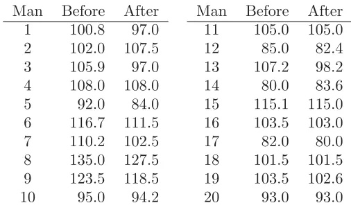
2.2 The weights, in kilograms, of twenty men before and after participation in a ‘waist loss’ program are shown in Table 2.8. (Egger et al., 1999) We want to know if, on average, they retain a weight loss twelve months after the program.

Table 2.8 Weights of twenty men before and after participation in a ‘waist loss’ program.

Man Before After Man Before After

1 100.8 97.0 11 105.0 105.0

2 102.0 107.5 12 85.0 82.4

3 105.9 97.0 13 107.2 98.2

4 108.0 108.0 14 80.0 83.6

5 92.0 84.0 15 115.1 115.0

6 116.7 111.5 16 103.5 103.0

7 110.2 102.5 17 82.0 80.0

8 135.0 127.5 18 101.5 101.5

9 123.5 118.5 19 103.5 102.6

10 95.0 94.2 20 93.0 93.0

Let Y_jk denote the weight of the kth man at the jth time where j = 1 before the program and j = 2 twelve months later. Assume the Y_jk’s are independent random variables with Y_jk ∼ N(μ_j, σ2) for j = 1,2 and

k= 1, ...,20.

(a) Use an unpaired t-test to test the hypothesis

H₀:μ₁=μ₂ versus H₁:μ₁=μ₂.

(b) Let D_k = Y_1k−Y_2k, fork = 1, ...,20. Formulate models for testing H₀ against H₁ using the D_k’s. Using analogous methods to Exercise 2.1 above, assumingσ2 is a known constant, test H₀ against H₁.

(d) List the assumptions made for (a) and (b). Which analysis is more appropriate for these data?

2.3 For model (2.7) for the data on birthweight and gestational age, using methods similar to those for Exercise 1.4, show

S₁ =

J

j=1 K

k=1

(Y_jk−a_j−b_jx_jk)2

=

J

j=1 K

k=1

[(Y_jk−(α_j+β_jx_jk)]2−K

J

j=1

(Y_j−α_j−β_jx_j)2

− J

j=1

(b_j−β_j)2(

K

k=1 x2

jk−Kx2j)

and that the random variablesY_jk,Y_j andb_j are all independent and have the following distributions

Y_{jk ∼} N(α_j+β_jx_jk, σ2),

Y_{j ∼} N(α_j+β_jx_j, σ2/K),

b_{j ∼} N(β_j, σ2/(

K

k=1 x2

jk−Kx2j)).

2.4 Suppose you have the following data

x: 1.0 1.2 1.4 1.6 1.8 2.0

y: 3.15 4.85 6.50 7.20 8.25 16.50

and you want to fit a model with

E(Y) = ln(β₀+β₁x+β₂x2).

Write this model in the form of (2.13) specifying the vectorsy and β and the matrixX.

2.5 The model for two-factor analysis of variance with two levels of one factor, three levels of the other and no replication is

E(Y_jk) =μ_jk =μ+α_j+β_k; Y_jk ∼N(μ_jk, σ2)

wherej = 1,2;k= 1,2,3 and, using the sum-to-zero constraints,α₁+α₂ = 0, β₁+β₂+β₃ = 0.Also the Y_jk’s are assumed to be independent. Write the equation for E(Y_jk) in matrix notation. (Hint: let α₂ = −α₁, and