What is Statistical Learning?
0 50 100 200 300
5
10
15
20
25
TV
Sales
0 10 20 30 40 50
5
10
15
20
25
Radio
Sales
0 20 40 60 80 100
5
10
15
20
25
Newspaper
Sales
Shown areSales vsTV,Radio andNewspaper, with a blue linear-regression line fit separately to each.
Can we predictSalesusing these three? Perhaps we can do better using a model
Notation
HereSales is aresponseortarget that we wish to predict. We generically refer to the response asY.
TVis afeature, orinput, orpredictor; we name itX1.
Likewise nameRadioasX2, and so on.
We can refer to theinput vectorcollectively as
X=
X1 X2 X3
Now we write our model as
Y =f(X) +
What is
f
(
X
) good for?
• With a good f we can make predictions of Y at new points X =x.
• We can understand which components of
X = (X1, X2, . . . , Xp) are important in explainingY, and
which are irrelevant. e.g. Seniority and Years of Education have a big impact on Income, butMarital Statustypically does not.
● ● ● ● ● ● ● ● ● ● ● ● ● ● ● ● ● ● ● ● ● ● ● ● ● ● ● ● ●● ● ● ● ● ● ● ● ● ● ● ● ● ● ● ● ● ● ● ● ● ● ● ● ● ● ● ● ● ● ●● ● ● ● ● ● ● ● ● ● ● ● ● ● ● ● ● ● ●● ● ● ● ● ● ● ● ● ● ● ● ● ● ● ● ● ● ● ● ● ● ● ● ● ● ● ● ● ● ● ● ● ● ● ● ● ● ● ● ● ● ● ● ● ● ● ● ● ● ● ● ● ● ● ● ● ● ● ● ● ● ● ● ● ● ● ● ● ● ● ● ● ● ● ● ● ● ● ● ● ● ● ● ● ● ● ● ● ● ● ● ● ● ● ● ● ● ● ● ● ● ● ● ● ● ● ● ● ● ● ● ● ● ● ● ● ● ● ● ●● ● ● ● ● ● ● ● ● ● ● ● ● ● ● ● ● ● ● ● ● ● ● ● ● ● ● ● ● ● ● ● ● ● ● ● ● ● ● ● ● ● ● ● ● ● ● ● ● ● ● ● ● ● ● ● ● ● ● ● ● ● ● ● ● ● ● ● ● ● ● ● ● ● ● ● ● ● ● ● ● ● ● ● ● ● ● ● ● ● ● ● ● ● ● ● ● ● ● ● ● ● ● ● ● ● ● ● ● ● ● ● ● ● ● ● ● ● ● ● ● ● ● ● ● ● ● ● ● ● ● ● ● ● ● ● ● ● ● ● ● ● ● ● ● ● ● ● ● ● ● ● ● ● ● ● ● ● ● ● ● ● ● ● ● ● ● ● ● ● ● ● ● ● ● ● ● ● ● ● ● ● ● ● ● ● ● ● ● ● ● ● ● ● ● ● ● ● ● ● ● ● ● ● ● ● ● ● ● ● ● ● ● ● ● ● ● ● ● ● ● ● ● ● ● ● ● ● ● ● ● ● ● ● ● ● ● ● ● ● ● ● ● ● ● ● ● ● ● ● ● ● ● ● ● ● ● ● ● ● ● ● ● ● ● ● ● ● ● ● ● ● ● ● ● ● ● ● ● ● ●● ● ● ● ● ● ● ● ● ● ● ● ● ● ● ● ● ● ● ● ● ● ● ● ● ● ● ● ● ● ● ● ● ● ● ● ●● ● ● ● ● ● ● ● ● ● ● ● ● ● ● ● ● ● ● ● ● ● ● ● ● ● ● ● ● ● ● ● ● ● ● ● ● ● ● ● ● ● ● ● ● ● ● ● ● ● ● ● ● ● ● ● ● ● ● ● ● ● ● ● ● ● ●● ● ● ● ● ● ● ● ● ● ● ● ● ● ● ● ● ● ● ● ● ● ● ● ● ●●● ● ● ● ● ● ● ● ● ● ● ● ● ● ● ● ● ● ●● ● ● ● ● ● ● ● ● ● ● ● ● ● ● ● ● ● ● ● ● ● ● ● ● ● ● ● ● ● ● ● ● ● ●● ● ● ● ● ● ● ● ● ● ● ● ● ●● ● ● ● ● ● ● ● ● ● ● ● ● ● ● ● ● ● ● ● ● ● ● ● ● ● ● ● ● ● ● ● ● ● ● ● ● ● ● ● ● ● ● ● ● ● ● ● ● ● ● ● ● ● ● ● ● ● ● ● ● ● ● ● ● ● ● ● ● ● ● ● ● ● ● ● ● ● ● ● ● ● ● ● ● ● ● ● ●● ● ● ● ● ● ● ● ● ● ● ● ● ● ● ● ● ● ● ● ● ● ● ● ● ● ● ● ● ● ● ● ● ● ● ● ● ● ● ● ● ● ● ● ● ● ● ● ● ● ● ● ● ● ● ● ● ● ● ● ● ● ● ● ● ● ● ● ● ● ● ● ● ● ●● ● ● ● ● ● ● ● ● ● ● ● ● ● ● ● ● ● ● ● ● ● ● ● ● ● ● ● ● ● ● ● ● ● ● ● ● ● ● ● ● ● ● ● ● ● ● ● ● ● ● ● ● ● ● ● ● ● ● ● ● ● ● ● ● ● ● ● ● ● ● ● ● ●● ● ● ● ● ● ● ● ● ● ● ● ● ● ● ● ● ● ● ● ● ● ● ● ● ● ● ● ● ● ● ● ● ● ● ● ● ● ● ● ● ● ● ● ● ● ● ● ● ● ● ● ● ● ● ● ● ● ● ● ● ● ● ● ● ● ● ● ● ● ● ● ● ● ● ● ● ● ● ● ● ● ● ● ● ● ● ● ● ● ● ● ● ● ● ● ● ● ● ● ● ● ● ● ● ● ● ● ● ● ● ● ● ● ● ● ● ● ● ● ● ● ● ● ● ● ● ● ● ● ● ● ● ● ● ● ● ●● ● ● ● ● ● ●● ● ● ● ● ● ● ● ● ● ● ● ● ● ● ● ● ● ● ● ● ● ● ● ● ● ● ● ● ● ● ● ● ● ● ● ● ● ● ● ● ● ● ● ● ● ● ● ● ● ● ●● ● ● ● ●● ● ● ● ● ● ●● ● ● ● ● ● ● ● ● ● ● ● ● ● ●● ● ● ● ● ● ● ● ● ● ● ●● ● ● ● ● ● ● ● ● ● ● ● ● ● ● ● ● ● ● ● ● ● ● ● ● ● ● ● ● ● ● ● ● ● ● ● ● ● ● ● ● ● ● ● ● ● ● ● ● ● ● ● ● ● ● ● ● ● ● ● ● ● ● ● ● ● ● ● ● ● ● ● ● ● ● ● ● ● ● ● ● ● ● ● ● ● ● ● ● ● ● ● ● ● ● ● ● ● ● ● ● ● ● ●● ● ● ● ● ● ● ● ● ● ● ● ● ● ● ● ● ● ● ● ● ● ● ● ● ● ●● ● ● ● ● ● ● ● ● ● ●● ● ● ● ● ● ● ● ● ● ● ●● ● ● ● ● ● ● ● ● ● ● ● ● ● ● ● ● ● ● ● ● ● ● ● ● ● ● ● ● ● ● ● ● ● ● ● ● ● ● ● ● ● ● ● ● ● ● ● ● ●● ● ● ● ● ● ● ● ● ● ● ● ● ● ● ● ● ● ● ●● ● ● ● ● ● ● ● ● ● ● ● ● ● ● ● ● ● ● ● ● ● ● ● ● ● ● ● ● ● ● ● ● ● ● ● ● ● ● ● ● ● ● ● ● ● ● ● ● ● ● ● ● ● ● ● ● ● ● ● ● ● ● ● ● ● ● ● ● ● ● ● ● ● ● ● ● ● ● ● ● ● ● ● ● ● ● ● ● ● ● ● ● ● ●● ● ● ● ● ● ● ● ● ● ● ● ● ● ● ● ● ● ● ● ● ● ● ● ● ● ● ● ● ● ● ● ● ● ● ● ● ● ● ● ● ● ● ● ● ● ● ● ● ● ● ● ● ● ● ● ● ● ● ● ● ● ● ● ● ● ● ● ● ● ● ● ● ● ● ● ● ● ● ● ● ● ● ● ● ● ● ● ● ● ● ● ● ● ● ● ● ● ● ● ● ●● ● ● ● ● ● ● ● ● ● ● ● ● ● ● ● ● ● ● ● ● ● ● ● ● ● ● ● ● ● ● ● ● ● ● ● ● ● ● ●● ● ● ● ● ● ● ● ● ● ● ● ● ● ● ● ● ● ● ● ● ● ● ● ● ● ● ● ● ● ● ● ● ● ● ● ● ● ● ● ● ● ● ● ● ● ● ● ● ● ● ● ● ● ● ● ● ● ● ● ● ● ● ● ● ● ●● ● ● ● ● ● ● ● ● ● ● ● ● ● ● ● ● ● ● ● ● ● ● ● ● ● ● ● ● ● ● ● ● ● ● ● ● ●● ● ● ● ● ● ● ● ● ● ● ● ● ● ● ● ● ● ● ● ● ● ● ● ● ● ● ● ● ● ● ● ● ● ● ● ● ● ● ● ● ● ● ● ● ● ● ● ● ● ● ● ● ● ● ● ● ● ● ● ● ● ● ● ● ● ● ● ● ● ● ● ● ● ● ● ● ● ● ● ● ● ● ● ● ● ● ● ● ● ● ● ● ● ● ● ● ● ● ● ● ● ● ● ● ● ● ● ● ● ● ● ● ● ● ● ● ● ● ● ● ● ● ● ● ● ● ● ● ● ● ● ● ● ● ● ● ● ● ● ● ● ● ● ● ● ● ● ● ● ● ● ● ● ● ● ● ● ● ● ● ● ● ● ● ● ● ● ● ● ● ● ● ● ● ● ● ● ● ● ● ● ● ● ● ● ● ● ● ● ● ● ● ● ● ● ● ●● ● ● ● ● ● ● ● ● ● ● ● ● ● ● ● ● ● ● ● ● ● ● ● ● ● ● ● ● ● ● ● ● ● ● ● ●● ● ● ● ● ● ● ● ● ● ● ● ● ● ● ● ● ● ● ● ● ●● ● ● ● ● ● ● ● ● ● ● ● ● ● ● ● ● ● ● ● ● ● ●
1 2 3 4 5 6 7
−2 0 2 4 6 x y ●
Is there an idealf(X)? In particular, what is a good value for f(X) at any selected value of X, sayX = 4? There can be manyY values atX = 4. A good value is
f(4) =E(Y|X = 4)
E(Y|X= 4) meansexpected value(average) ofY given X= 4.
The regression function
f
(
x
)
• Is also defined for vectorX; e.g.
f(x) =f(x1, x2, x3) =E(Y|X1=x1, X2 =x2, X3 =x3)
• Is theidealoroptimal predictor of Y with regard to mean-squared prediction error: f(x) =E(Y|X=x) is the function that minimizesE[(Y −g(X))2|X =x] over all functions g at all points X=x.
• =Y −f(x) is the irreducibleerror — i.e. even if we knew f(x), we would still make errors in prediction, since at each X =x there is typically a distribution of possibleY values. • For any estimate ˆf(x) off(x), we have
E[(Y −fˆ(X))2|X =x] = [f(x)−fˆ(x)]2
| {z }
Reducible
+ Var() | {z }
The regression function
f
(
x
)
• Is also defined for vectorX; e.g.
f(x) =f(x1, x2, x3) =E(Y|X1=x1, X2 =x2, X3 =x3)
• Is theidealoroptimal predictor of Y with regard to mean-squared prediction error: f(x) =E(Y|X=x) is the function that minimizesE[(Y −g(X))2|X =x] over all functions g at all points X=x.
• =Y −f(x) is the irreducibleerror — i.e. even if we knew f(x), we would still make errors in prediction, since at each X =x there is typically a distribution of possibleY values.
• For any estimate ˆf(x) off(x), we have E[(Y −fˆ(X))2|X =x] = [f(x)−fˆ(x)]2
| {z }
Reducible
+ Var() | {z }
The regression function
f
(
x
)
• Is also defined for vectorX; e.g.
f(x) =f(x1, x2, x3) =E(Y|X1=x1, X2 =x2, X3 =x3)
• Is theidealoroptimal predictor of Y with regard to mean-squared prediction error: f(x) =E(Y|X=x) is the function that minimizesE[(Y −g(X))2|X =x] over all functions g at all points X=x.
• =Y −f(x) is the irreducibleerror — i.e. even if we knew f(x), we would still make errors in prediction, since at each X =x there is typically a distribution of possibleY values. • For any estimate ˆf(x) off(x), we have
E[(Y −fˆ(X))2|X =x] = [f(x)−fˆ(x)]2
| {z }
Reducible
+ Var() | {z }
How to estimate
f
• Typically we have few if any data points with X= 4 exactly.
• So we cannot compute E(Y|X =x)! • Relax the definition and let
ˆ
f(x) = Ave(Y|X∈ N(x))
where N(x) is someneighborhood of x.
● ●
● ●
● ● ●
●
●
● ●
●
●
● ●
● ●
● ● ●
● ●
● ●
●
●
●
● ●
● ●
● ●
●
●
●
● ●
●
● ●
●
●
● ●
● ●
● ● ●
● ●
● ●
●
●
●
● ●
● ●
● ● ●
●
● ●
● ● ●
1 2 3 4 5 6
−2
−1
0
1
2
3
x
y
• Nearest neighbor averaging can be pretty good for small p — i.e. p≤4 and large-ishN.
• We will discuss smoother versions, such as kernel and spline smoothing later in the course.
• Nearest neighbor methods can be lousywhen pis large. Reason: the curse of dimensionality. Nearest neighbors tend to be far away in high dimensions.
• We need to get a reasonable fraction of theN values ofyi
to average to bring the variance down—e.g. 10%.
• Nearest neighbor averaging can be pretty good for small p — i.e. p≤4 and large-ishN.
• We will discuss smoother versions, such as kernel and spline smoothing later in the course.
• Nearest neighbor methods can be lousywhen pis large. Reason: thecurse of dimensionality. Nearest neighbors tend to be far away in high dimensions.
• We need to get a reasonable fraction of theN values ofyi
to average to bring the variance down—e.g. 10%.
The curse of dimensionality
● ●
●
● ●
●
● ● ●
● ●
● ● ● ●
● ●
●
● ●
● ●
● ●
●
● ● ●
●
● ●
● ●
● ●
●
● ●
●
● ●
● ●
●
●
● ●
●
● ● ●
● ● ●
●
● ●
●
● ● ●
●
●
● ●
●
● ● ●
● ●
● ● ●
● ●
● ●
●
●
● ●
●
● ●
● ●
●
● ●
●
● ●
● ●
● ●
● ●
●
−1.0 −0.5 0.0 0.5 1.0
−1.0
−0.5
0.0
0.5
1.0
x1
x2
10% Neighborhood
●
0.0 0.1 0.2 0.3 0.4 0.5 0.6 0.7
0.0
0.5
1.0
1.5
Fraction of Volume
Radius
Parametric and structured models
Thelinear model is an important example of a parametric model:
fL(X) =β0+β1X1+β2X2+. . . βpXp.
• A linear model is specified in terms of p+ 1 parameters β0, β1, . . . , βp.
• We estimate the parameters by fitting the model to training data.
A linear model ˆfL(X) = ˆβ0+ ˆβ1X gives a reasonable fit here
● ●
● ●
● ● ● ●
● ●
● ●
●
● ●
● ●
● ● ●
● ● ● ●
●
●
● ●
● ●
● ●
●
●
●
● ●
● ●
● ●
●
●
● ●
● ● ●
● ●
● ●
● ●
●
●
● ●
●
● ●
● ● ●
● ● ●
● ● ●
1 2 3 4 5 6
−2
−1
0
1
2
3
x
y
●
A quadratic model ˆfQ(X) = ˆβ0+ ˆβ1X+ ˆβ2X2 fits slightly
better.
● ●
● ●
● ● ● ●
● ●
● ●
●
● ●
● ●
● ● ●
● ● ● ●
●
●
● ● ● ●
● ●
●
●
●
● ●
● ●
● ●
●
●
● ●
● ● ●
● ●
● ●
● ●
●
●
● ●
●
● ●
● ● ●
● ● ●
● ● ●
1 2 3 4 5 6
−2
−1
0
1
2
3
x
y
Years of Education
Senior ity
Income
Simulated example. Red points are simulated values forincome from the model
income=f(education,seniority) +
Years of Education
Senior ity
Income
Linear regression model fit to the simulated data.
ˆ
Years of Education
Senior ity
Income
More flexible regression model ˆfS(education,seniority) fit to
Years of Education
Senior ity
Income
Even more flexible spline regression model ˆ
fS(education,seniority) fit to the simulated data. Here the
Some trade-offs
• Prediction accuracy versus interpretability.
— Linear models are easy to interpret; thin-plate splines are not.
• Good fit versus over-fit or under-fit.
— How do we know when the fit is just right? • Parsimony versus black-box.
Some trade-offs
• Prediction accuracy versus interpretability.
— Linear models are easy to interpret; thin-plate splines are not.
• Good fit versus over-fit or under-fit.
— How do we know when the fit is just right?
• Parsimony versus black-box.
Some trade-offs
• Prediction accuracy versus interpretability.
— Linear models are easy to interpret; thin-plate splines are not.
• Good fit versus over-fit or under-fit.
— How do we know when the fit is just right? • Parsimony versus black-box.
2.1 What Is Statistical Learning? 25
Flexibility
Inter
pretability
Low High
Lo
w
High
Subset Selection Lasso
Least Squares
Generalized Additive Models Trees
Bagging, Boosting
Support Vector Machines
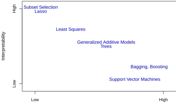
FIGURE 2.7. A representation of the tradeoff between flexibility and inter-pretability, using different statistical learning methods. In general, as the flexibil-ity of a method increases, its interpretabilflexibil-ity decreases.
more interpretable. For instance, when inference is the goal, the linear model may be a good choice since it will be quite easy to understand
the relationship between Y and X1, X2, . . . , Xp. In contrast, very flexible
approaches, such as the splines discussed in Chapter 7 and displayed in Figures 2.5 and 2.6, and the boosting methods discussed in Chapter 8, can
lead to such complicated estimates of f that it is difficult to understand
how any individual predictor is associated with the response.
Figure 2.7 provides an illustration of the trade-off between flexibility and interpretability for some of the methods that we cover in this book. Least squares linear regression, discussed in Chapter 3, is relatively inflexible but
is quite interpretable. The lasso, discussed in Chapter 6, relies upon the
lasso
linear model (2.4) but uses an alternative fitting procedure for estimating
the coefficients β0, β1, . . . , βp. The new procedure is more restrictive in
es-timating the coefficients, and sets a number of them to exactly zero. Hence in this sense the lasso is a less flexible approach than linear regression. It is also more interpretable than linear regression, because in the final model the response variable will only be related to a small subset of the
predictors — namely, those with nonzero coefficient estimates.Generalized
additive models (GAMs), discussed in Chapter 7, instead extend the
lin-generalized additive model
ear model (2.4) to allow for certain non-linear relationships. Consequently, GAMs are more flexible than linear regression. They are also somewhat less interpretable than linear regression, because the relationship between each predictor and the response is now modeled using a curve. Finally, fully
Assessing Model Accuracy
Suppose we fit a model ˆf(x) to some training data
Tr={xi, yi}N1 , and we wish to see how well it performs.
• We could compute the average squared prediction error overTr:
MSETr= Avei∈Tr[yi−fˆ(xi)]2
This may be biased toward more overfit models.
• Instead we should, if possible, compute it using fresh test
data Te={xi, yi}M1 :
2.2 Assessing Model Accuracy 31
0 20 40 60 80 100
2
4
6
8
10
12
X
Y
2 5 10 20
0.0
0.5
1.0
1.5
2.0
2.5
Flexibility
Mean Squared Error
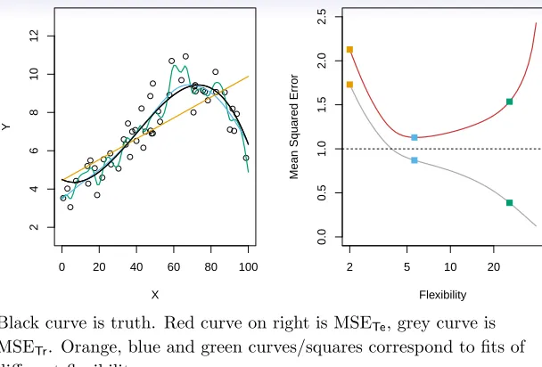
FIGURE 2.9.Left:Data simulated fromf, shown in black. Three estimates of
f are shown: the linear regression line (orange curve), and two smoothing spline fits (blue and green curves). Right: Training MSE (grey curve), test MSE (red curve), and minimum possible test MSE over all methods (dashed line). Squares represent the training and test MSEs for the three fits shown in the left-hand panel.
statistical methods specifically estimate coefficients so as to minimize the training set MSE. For these methods, the training set MSE can be quite small, but the test MSE is often much larger.
Figure 2.9 illustrates this phenomenon on a simple example. In the left-hand panel of Figure 2.9, we have generated observations from (2.1) with the truef given by the black curve. The orange, blue and green curves illus-trate three possible estimates forf obtained using methods with increasing levels of flexibility. The orange line is the linear regression fit, which is rela-tively inflexible. The blue and green curves were produced usingsmoothing
splines, discussed in Chapter 7, with different levels of smoothness. It is
smoothing spline
clear that as the level of flexibility increases, the curves fit the observed data more closely. The green curve is the most flexible and matches the data very well; however, we observe that it fits the truef (shown in black) poorly because it is too wiggly. By adjusting the level of flexibility of the smoothing spline fit, we can produce many different fits to this data.
We now move on to the right-hand panel of Figure 2.9. The grey curve displays the average training MSE as a function of flexibility, or more for-mally the degrees of freedom, for a number of smoothing splines. The
de-degrees of freedom
grees of freedom is a quantity that summarizes the flexibility of a curve; it is discussed more fully in Chapter 7. The orange, blue and green squares
Black curve is truth. Red curve on right is MSETe, grey curve is MSETr. Orange, blue and green curves/squares correspond to fits of different flexibility.
2.2 Assessing Model Accuracy 33
0 20 40 60 80 100
2
4
6
8
10
12
X
Y
2 5 10 20
0.0
0.5
1.0
1.5
2.0
2.5
Flexibility
Mean Squared Error
FIGURE 2.10. Details are as in Figure 2.9, using a different true f that is much closer to linear. In this setting, linear regression provides a very good fit to the data.
0 20 40 60 80 100
−10
0
10
20
X
Y
2 5 10 20
0
5
10
15
20
Flexibility
Mean Squared Error
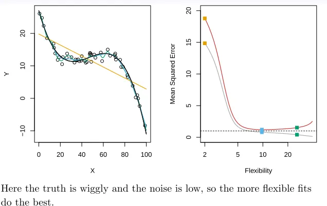
FIGURE 2.11.Details are as in Figure 2.9, using a differentfthat is far from linear. In this setting, linear regression provides a very poor fit to the data.
Here the truth is smoother, so the smoother fit and linear model do really well.
2.2 Assessing Model Accuracy 33
0 20 40 60 80 100
2
4
6
8
10
12
X
Y
2 5 10 20
0.0
0.5
1.0
1.5
2.0
2.5
Flexibility
Mean Squared Error
FIGURE 2.10. Details are as in Figure 2.9, using a different true f that is much closer to linear. In this setting, linear regression provides a very good fit to the data.
0 20 40 60 80 100
−10
0
10
20
X
Y
2 5 10 20
0
5
10
15
20
Flexibility
Mean Squared Error
FIGURE 2.11.Details are as in Figure 2.9, using a differentfthat is far from linear. In this setting, linear regression provides a very poor fit to the data.
Bias-Variance Trade-off
Suppose we have fit a model ˆf(x) to some training data Tr, and let (x0, y0) be a test observation drawn from the population. If
the true model isY =f(X) +(with f(x) =E(Y|X=x)), then
Ey0−fˆ(x0) 2
= Var( ˆf(x0)) + [Bias( ˆf(x0))]2+ Var().
The expectation averages over the variability ofy0 as well as
the variability inTr. Note that Bias( ˆf(x0))] =E[ ˆf(x0)]−f(x0).
Bias-variance trade-off for the three examples
36 2. Statistical Learning
2 5 10 20
0.0
0.5
1.0
1.5
2.0
2.5
Flexibility
2 5 10 20
0.0
0.5
1.0
1.5
2.0
2.5
Flexibility
2 5 10 20
0
5
10
15
20
Flexibility MSE Bias Var
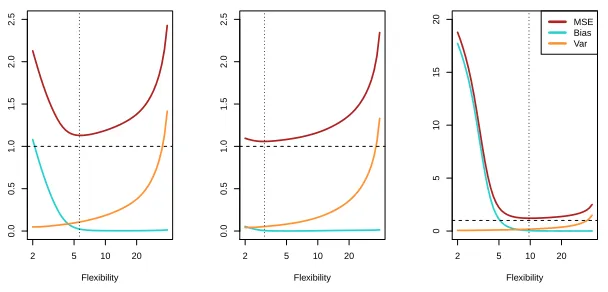
FIGURE 2.12. Squared bias (blue curve), variance (orange curve), Var(ǫ)
(dashed line), and test MSE (red curve) for the three data sets in Figures 2.9–2.11. The vertical dashed line indicates the flexibility level corresponding to the smallest test MSE.
ibility increases, and the test MSE only declines slightly before increasing rapidly as the variance increases. Finally, in the right-hand panel of Fig-ure 2.12, as flexibility increases, there is a dramatic decline in bias because
the truef is very non-linear. There is also very little increase in variance
as flexibility increases. Consequently, the test MSE declines substantially before experiencing a small increase as model flexibility increases.
The relationship between bias, variance, and test set MSE given in
Equa-tion 2.7 and displayed in Figure 2.12 is referred to as the bias-variance
trade-off. Good test set performance of a statistical learning method
re-bias-variance trade-off quires low variance as well as low squared bias. This is referred to as a
trade-off because it is easy to obtain a method with extremely low bias but high variance (for instance, by drawing a curve that passes through every single training observation) or a method with very low variance but high bias (by fitting a horizontal line to the data). The challenge lies in finding a method for which both the variance and the squared bias are low. This trade-off is one of the most important recurring themes in this book.
In a real-life situation in whichf is unobserved, it is generally not
pos-sible to explicitly compute the test MSE, bias, or variance for a statistical learning method. Nevertheless, one should always keep the bias-variance trade-off in mind. In this book we explore methods that are extremely flexible and hence can essentially eliminate bias. However, this does not guarantee that they will outperform a much simpler method such as linear
regression. To take an extreme example, suppose that the truefis linear.
In this situation linear regression will have no bias, making it very hard
for a more flexible method to compete. In contrast, if the truefis highly
non-linear and we have an ample number of training observations, then we may do better using a highly flexible approach, as in Figure 2.11. In
Classification Problems
Here the response variableY isqualitative — e.g. email is one ofC= (spam,ham) (ham=good email), digit class is one of
C={0,1, . . . ,9}. Our goals are to:
• Build a classifier C(X) that assigns a class label fromC to a future unlabeled observation X.
• Assess the uncertainty in each classification
| | | | | | | | | | | | | | | | | | | | | | | | | | | | || | | | | | | | | | || | | | | | | | | | | | | | | | | || | | | | | || | | || | | | | | | | | | | | | || | | | | || | | | | | | | | | | | | | | | | | | | | | | | | | | | |||| | | | | || | | | | | | | | | | | | | | | | | | | | | || | | | | | | | | | | | | | | | | | | | | | | | | | | | | | | | | | || | | || | || | | || | | | | | | | | | | | | | | | | | | | | | | | | || | | | | | | | | | | | | | | | | | | | | | | | | | | || | | | | | | | | | || | | | | | | | | | | | | | | | | | | | | | | | | | | | | | | | | | | | | | | | | | | | | | | | | | | | | | | | | | | | | | | | | | || | | | | | | | | | | | | | | | | | | | | | | | | | | | | || | | || | | | | | | | | | | | | | | | | | | | | | | | | | | | | | | | | | | | | | | | | | | | | | | | | | | | | | | | | | | || | | | | | | | | | | | | | | | | | | | | | | | | | | | | | | | | | | | | | | | | | | | | | | | | | | | | | | | | | | | || | | | || | | | | | | | | | | | | | || | | | | | | | | | | | | | | | | | | | | | | | | | | | | | | | | | | | | | | | | | | | | || | | | | | | | | | | | | | | | | | | | | | | | | | | | || | | | | | || | | | | | | | | | | | | | | | | | | | | | || | | | | | | | | || | | | | | | | | | ||| || | | | | | | | | | | | | | | | | || | | | | | | | | | | | | | | | | | | | | | | | | | || | | | | | | || | | | | | | | | | | | | | | | | | | | | | | | | | | | | | | | | | | | | | | | | | | | | | | | | | | | | | | | | | | | | | | | | | | | | | | | | | | || | | | | | | | | | | | | | | | | | || | | | | | | | | | | | |||||| | | | | || | | | | | | | | | | | | | | | | | | || | | | | | | | | | | | | | | | | | | | | | | | | | | | | | | | | | | | | | | | | | | | | | | | | | | | | | | | | | | | | | | | | | | | | | | | | | | | | | | || | | | | | | | | | | | | | | | | | | | | | | | | | | | | | | | | | | | | | | | | | | | | | | | | | | | | | | | | | | | | | | | | | | | | | | | | | | | | | | | | | | | | | | | | | | | | | | | | | | | | | | | | | | | | | | | | | | | | | | | | | | | | | | | | | | | | | | | | | | | | | | | | | | | | | | | | | | | | | | | | | | | | || | | || | | | | | | | | | | | | | | | | | | | | | | | | | | | | | | | | | | | | | | | | || || | | | | | | | | | | | || | | | | | | | | | | | | | | | | | | | | | | | || | | | | | | | | | | | | | | | | | | | | | | | | | | | | | | | | | | | | | | | | || | | | | | | | | | | | | | | | | | | | | | | | | | | | | | | | | | | | | | | | | | | | | | | | | | | | | | || | | | | | | | | | | | | | | | | | | | | | | | | | | | | | | | | | | | | | | | | | | | | | | | | | | | || | | | |||| | | | | | | | | | | | | | | | | | | | | | | | | | | | | | | | | | | | | | | | | | | | | | || | | | | | | | | | | | | | | | | | | | | | | | | | | | | | | | | | | | | | | | | || | | | | | | | | | | | | | | | | | | | | | | | || | | | | | | | | | | | | | | | | | | | | | | | | | | | | | | | | | | | | | | | | | | | | | | | | | | | | | | || | | | | | | | | | | | | | | | | | | | | | | | | | | | | | | | | | | | | | | | | | || | || | | | | | | || | | | | | | | | | | | | | | | | | | | | | | | | | | | | | | | | | | | | | | | | | | | | | | | | | | | | | | | | | | | | | | | | | | | | | | | | | | | | | | || | | | | | | | | | | | | | | | | | | | | | | | | | | | | | | | | | | | | | | | | | | | | | | | | | | | | | | | | | | | | || | | | || | | | | | | | | | | | | | | | | | | | | | | | | | | | | | | | | | | | | | | | | | | ||| | | | | | | | | | | | | | | | | | | | | | | | | | | | | | | | | | | | | | | | | | | | | | | | | | | | | | | | | | | | | | | | | | | | | | | | | | | | | | | | | | | | | | | | | | | | | | | | | | | | | || | | | | | | | | | | | | | | | | | | | | | | | | | | | | | | | | | | | | || | | | | | | | | | | | | | | | | | | | | | | | | | | | | | | | | | | | | | | | | | | | | | | | | | || | | | | | | | | | | | | | | | | | | | | | | | | | | | | | | | | | | | | | | | | | | | | | | | | | | | | | | | | | | | | | | | | | | | | | | | | | | | | | | | | |
1 2 3 4 5 6 7
0.0 0.2 0.4 0.6 0.8 1.0 x y
Is there an idealC(X)? Suppose the K elements inC are numbered 1,2, . . . , K. Let
pk(x) = Pr(Y =k|X =x), k= 1,2, . . . , K.
These are theconditional class probabilitiesatx; e.g. see little barplot atx= 5. Then theBayes optimalclassifier at x is
|
|
| |
|
|
|
|
| |
|
|
|
|
|
|
|
| |
| | |
| |
| |
|
|
||
|
| |
|
|
|
| |
|
||
|
| | | | | |
|
| |
|
|
|
|
| |
|| | |
| |
| |
|
|
| ||
| |
|
|
| | | |
|
| | |
| |
| |
|
|
|
| |
| | |
|
| | |
| |
2 3 4 5 6
0.0
0.2
0.4
0.6
0.8
1.0
x
y
Nearest-neighbor averaging can be used as before.
Also breaks down as dimension grows. However, the impact on ˆ
Classification: some details
• Typically we measure the performance of ˆC(x) using the misclassification error rate:
ErrTe = Avei∈TeI[yi 6= ˆC(xi)]
• The Bayes classifier (using the true pk(x)) has smallest
error (in the population).
• Support-vector machines build structured models forC(x). • We will also build structured models for representing the
Example: K-nearest neighbors in two dimensions
38 2. Statistical Learningo o
o
o o
o o
o
o
o
o
o
o
o o
o o
o o
o o
o
oo o
o
o o
o o o
o
o
o
o
o
o o
o o
o o
o
o
o
o o
o
o
o o o
o
o o o
o
o
o o
o o
o o
o o
o o o
o
o
o
o
o
o o o
o
o o
o o o
o o
o o
o
o o
o
o
o o
o
o o
o o
o o
o o
o o o
o
o
o
o
o
o
o o
o o
o
o
o o
o o
o o
o o
o
o o
o o
o o o
o o
o
o
o o
o
o
o
o o
o
o o
o o o o
o
o o
o o
o
o
o o
o
o o o
o
o
o o
o o
o
o
o o
o
o o
o
o o
o
o o o
o o
o o
o
o o
o
o
o o
o
o
o o
X1
X2
FIGURE 2.13.A simulated data set consisting of 100 observations in each of two groups, indicated in blue and in orange. The purple dashed line represents the Bayes decision boundary. The orange background grid indicates the region in which a test observation will be assigned to the orange class, and the blue background grid indicates the region in which a test observation will be assigned to the blue class.
only two possible response values, say
class 1
or
class 2
, the Bayes classifier
corresponds to predicting class one if Pr(
Y
= 1
|
X
=
x
0)>
0
.
5, and class
two otherwise.
Figure 2.13 provides an example using a simulated data set in a
two-dimensional space consisting of predictors
X
1and
X
2. The orange andblue circles correspond to training observations that belong to two different
classes. For each value of
X
1and
X
2, there is a different probability of theresponse being orange or blue. Since this is simulated data, we know how
the data were generated and we can calculate the conditional probabilities
for each value of
X
1and
X
2. The orange shaded region reflects the set ofpoints for which Pr(
Y
= orange
|
X
) is greater than 50%, while the blue
shaded region indicates the set of points for which the probability is below
50%. The purple dashed line represents the points where the probability
is exactly 50%. This is called the
Bayes decision boundary
. The Bayes
Bayes decision boundary
classifier’s prediction is determined by the Bayes decision boundary; an
observation that falls on the orange side of the boundary will be assigned
to the orange class, and similarly an observation on the blue side of the
boundary will be assigned to the blue class.
The Bayes classifier produces the lowest possible test error rate, called
the
Bayes error rate
. Since the Bayes classifier will always choose the class
Bayes error rate
for which (2.10) is largest, the error rate at
X
=
x
0will be 1
−
max
jPr(
Y
=
2.2 Assessing Model Accuracy 41 o o o o o o o o o o o o o o o o o o o o o o
oo o
o o o o o o o o o o o o o o o o o o o o o o o o
o o o
o o o o o o o o o o o o o o o o o o o o o o o o o o o o o o o o o o o o o o o o o o o o o o o o o o o o o o o o o o o o o o o o o o o o o o o o o o o o o o o o o o o o o o o o o o o o o o o o o o o o o o o o o o o o o o o o o o o o o o o o o o o o o o o o o o o o o o o o o o o o o o o o o o o o KNN: K=10 X1 X2
FIGURE 2.15. The black curve indicates the KNN decision boundary on the
data from Figure 2.13, using K = 10. The Bayes decision boundary is shown as
a purple dashed line. The KNN and Bayes decision boundaries are very similar.
o o o o o o o o o o o o o o o o o o o o o o oo o
o o o o o o o o o o o o o o o o o o o o o o o o
o o o o o o o o o o o o o o o o o o o o o o o o o o o o o o o o o o o o o o o o o o o o o o o o o o o o o o o o o o o o o o o o o o o o o o o o o o o o o o o o o o o o o o o o o o o o o o o o o o o o o o o o o o o o o o o o o o o o o o o o o o o o o o o o o o o o o o o o o o o o o o o o o o o o o o o o o o o o o o o o o o o o o o o o o o o o o oo o
o o o o o o o o o o o o o o o o o o o o o o o o
o o o o o o o o o o o o o o o o o o o o o o o o o o o o o o o o o o o o o o o o o o o o o o o o o o o o o o o o o o o o o o o o o o o o o o o o o o o o o o o o o o o o o o o o o o o o o o o o o o o o o o o o o o o o o o o o o o o o o o o o o o o o o o o o o o o o o o o o o o o o o o o o o o o o o o o
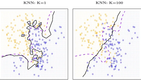
KNN: K=1 KNN: K=100
FIGURE 2.16. A comparison of the KNN decision boundaries (solid black
curves) obtained usingK = 1 and K = 100on the data from Figure 2.13. With
K = 1, the decision boundary is overly flexible, while with K = 100 it is not
sufficiently flexible. The Bayes decision boundary is shown as a purple dashed line.
2.2 Assessing Model Accuracy 41 o o o o o o o o o o o o o o o o o o o o o o
oo o
o o o o o o o o o o o o o o o o o o o o o o o o
o o o
o o o o o o o o o o o o o o o o o o o o o o o o o o o o o o o o o o o o o o o o o o o o o o o o o o o o o o o o o o o o o o o o o o o o o o o o o o o o o o o o o o o o o o o o o o o o o o o o o o o o o o o o o o o o o o o o o o o o o o o o o o o o o o o o o o o o o o o o o o o o o o o o o o o o KNN: K=10 X1 X2
FIGURE 2.15. The black curve indicates the KNN decision boundary on the
data from Figure 2.13, usingK = 10. The Bayes decision boundary is shown as
a purple dashed line. The KNN and Bayes decision boundaries are very similar.
o o o o o o o o o o o o o o o o o o o o o o oo o
o o o o o o o o o o o o o o o o o o o o o o o o
o o o o o o o o o o o o o o o o o o o o o o o o o o o o o o o o o o o o o o o o o o o o o o o o o o o o o o o o o o o o o o o o o o o o o o o o o o o o o o o o o o o o o o o o o o o o o o o o o o o o o o o o o o o o o o o o o o o o o o o o o o o o o o o o o o o o o o o o o o o o o o o o o o o o o o o o o o o o o o o o o o o o o o o o o o o o o oo o
o o o o o o o o o o o o o o o o o o o o o o o o
o o o o o o o o o o o o o o o o o o o o o o o o o o o o o o o o o o o o o o o o o o o o o o o o o o o o o o o o o o o o o o o o o o o o o o o o o o o o o o o o o o o o o o o o o o o o o o o o o o o o o o o o o o o o o o o o o o o o o o o o o o o o o o o o o o o o o o o o o o o o o o o o o o o o o o o
KNN: K=1 KNN: K=100
FIGURE 2.16. A comparison of the KNN decision boundaries (solid black
curves) obtained usingK = 1and K = 100 on the data from Figure 2.13. With
K = 1, the decision boundary is overly flexible, while with K = 100 it is not
sufficiently flexible. The Bayes decision boundary is shown as a purple dashed line.
42 2. Statistical Learning
0.01 0.02 0.05 0.10 0.20 0.50 1.00
0.00
0.05
0.10
0.15
0.20
1/K
Error Rate
Training Errors Test Errors
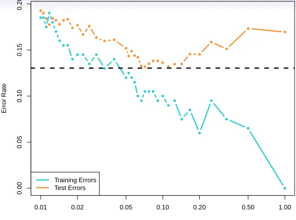
FIGURE 2.17.The KNN training error rate (blue, 200 observations) and test
error rate (orange, 5000 observations) on the data from Figure 2.13, as the level
of flexibility (assessed using 1/K) increases, or equivalently as the number of
neighborsK decreases. The black dashed line indicates the Bayes error rate. The
jumpiness of the curves is due to the small size of the training data set.
In both the regression and classification settings, choosing the correct level of flexibility is critical to the success of any statistical learning method. The bias-variance tradeoff, and the resulting U-shape in the test error, can make this a difficult task. In Chapter 5, we return to this topic and discuss various methods for estimating test error rates and thereby choosing the optimal level of flexibility for a given statistical learning method.
2.3 Lab: Introduction to R
In this lab, we will introduce some simple R commands. The best way to learn a new language is to try out the commands.Rcan be downloaded from
http://cran.r-project.org/
2.3.1 Basic Commands
Rusesfunctions to perform operations. To run a function calledfuncname,
function we typefuncname(input1, input2), where the inputs (orarguments)input1
argument