Earth Syst. Sci. Data, 10, 151–171, 2018 https://doi.org/10.5194/essd-10-151-2018 © Author(s) 2018. This work is distributed under the Creative Commons Attribution 4.0 License.
The Rofental: a high Alpine research basin
(1890–3770 m a.s.l.) in the Ötztal Alps (Austria) with over
150 years of hydrometeorological and glaciological
observations
Ulrich Strasser1, Thomas Marke1, Ludwig Braun3, Heidi Escher-Vetter3, Irmgard Juen2, Michael Kuhn2, Fabien Maussion2, Christoph Mayer3, Lindsey Nicholson2, Klaus Niedertscheider4,
Rudolf Sailer1, Johann Stötter1, Markus Weber5, and Georg Kaser2 1Department of Geography, University of Innsbruck, Innsbruck, 6020, Austria
2Department of Atmospheric and Cryospheric Sciences, University of Innsbruck, Innsbruck, 6020, Austria
3Geodesy and Glaciology, Bavarian Academy of Sciences and Humanities, Munich, 80539, Germany
4Hydrographic Service of Tyrol, Innsbruck, 6020, Austria
5Photogrammetry and Remote Sensing, Technical University of Munich, Munich, 80333, Germany
Correspondence:Ulrich Strasser ([email protected])
Received: 3 August 2017 – Discussion started: 21 August 2017
Revised: 26 November 2017 – Accepted: 18 December 2017 – Published: 24 January 2018
1 Introduction
Glaciers in the Rofental, Ötztal Alps, have been under obser-vation since the early 17th century; in particular the Vernagt-ferner (VF) was known for its dangerous surge-type advances (Richter, 1892) with flow velocities up to 11.5 m day−1 (Nicolussi, 2013). In 1599, the tongue of VF reached the valley floor of the Rofental, blocking the valley and form-ing an ice-dammed lake which burst, causform-ing a catastrophic lake outburst flood (GLOF) on 20 July in 1600. The painting of VF with its lake that was formed again in summer 1601 is the oldest known image of a glacier worldwide (Fig. 1). The lake was∼1700 m in length, and the lake level was at ∼2260 m a.s.l. (Nicolussi, 1990). Further advances of VF are documented for the periods around 1680, 1770 (the maxi-mum extent of VF in the little ice age, LIA), 1820 and 1848. Prior to the 19th century, each advance of VF formed the ice dam and lake in the Rofental, and the outflow of this lake was observed due to its dangerous nature (Nicolussi, 2013). The glacier changes were monitored with irregular glacier-front variation recordings.
A milestone in glacier cartography was the map “Der Ver-nagtferner im Jahre 1889 1 : 10 000”, constructed by means of terrestrial photogrammetry (Finsterwalder, 1897). This map showed, for the first time, an entire glacier in large scale with unprecedented details, including the area that became ice-free since the last glacier advance period (Fig. 2a). The first map of Hochjochferner (HJF) (1883) by Blümcke and Hess (1895) and Hintereisferner (HEF) (1894) by Blümcke and Hess (1899) followed shortly afterwards (Fig. 2b). Af-ter that, geodetic glacier maps were generated frequently for HEF, KWF and VF (Brunner, 2013; Charalampidis, 2018)1. These maps were accompanied by frequent terrestrial pho-tographs of VF between 1897 and 1928, documenting, for example, the last surge of the glacier (1897–1903). From these photographs Weber (2013) and Lindmayer (2015) re-constructed the extent and dynamics of VF for the respective periods. The monitoring of the geometry of the glaciers in the Rofental was accompanied by ice drilling experiments to reconstruct the glacier bed and dynamics (Blümcke and Hess, 1899), and first glacier flow theories were developed (Finsterwalder, 1897; Hess, 1904). With the foundation of the “International Commission for Snow and Ice” (ICSI) (as “International Glacier Commission” in Zürich 1894, re-named in 1948) the observation of glaciers became system-ized and internationally coordinated, and the continuous ob-servations of meteorological and hydrological variables be-gan: the first totalizing rain gauge in the Rofental was
in-1HEF: 1850, 1894, 1920, 1939, 1953, 1962, 1964, 1967, 1969,
1979, 1991, 1997, 2001–2008
KWF: 1939, 1967, 1969, 1979, 1991, 1997, 2001–2008
VF: 1846,1889, 1897, 1899, 1901, 1904, 1912, 1938, 1954, 1966, 1969, 1972,1979,1982,1990, 1994,1999, 2002, 2003,2006, 2009 (bold years available at http://geo.badw.de/vernagtferner-digital/ karten.html)
stalled in the village of Vent (1900 m a.s.l.) in 1905, fol-lowed by continuous measurements further up in the valley since 1952. The “Combined Water, Ice and Heat Balance Project in the Rofental” became an official initiative of the UNESCO International Hydrological Decade (IHD, 1964– 1974) (Hoinkes et al., 1974). Later, it was continued as part of the UNESCO International Hydrological Program (IHP) (http://en.unesco.org/themes/water-security/hydrology). Ab-lation stakes and pits for mass balance monitoring have been continuously maintained at HEF and Kesselwandferner (KWF) (since 1952), at VF (since 1965), and for short dis-continuous periods at HJF. As of 2017, the glacier mass bal-ance time series of HEF, VF and KWF are among the longest uninterrupted series worldwide (Fischer et al., 2015; Mayer et al., 2013a), and several automatic weather stations (AWSs) as well as runoff gauges at VF and in the village of Vent are in continuous operation. These are complemented by a network of historical rain gauges (totalizators) and modern precipita-tion gauges.
The comprehensive pool of long-term observations avail-able for the Rofental provides the basis for (i) manifold pro-cess studies on energy balance, ice dynamics, glacier hydrol-ogy and hydraulics (e.g., Kuhn et al., 1985a, b; Kuhn, 1987), (ii) new ground-based and remote sensing monitoring meth-ods (Escher-Vetter and Siebers, 2013; Juen et al., 2013; Hel-fricht et al., 2014a), (iii) model development and application in glaciological and regional hydrological research (Kaser et al., 2010; Escher-Vetter and Oerter, 2013; Schöber et al., 2014, 2016; Hanzer et al., 2016; Schmieder et al., 2016, 2018), (iv) the evaluation of potential future glacier evolu-tion and changes of the hydrological regime in a changing climate (Weber et al., 2009; Marke et al., 2013; Marzeion and Kaser, 2014; Weber and Prasch, 2015a, b; Hanzer et al., 2017), (v) attributing observed glacier changes to different drivers (Painter et al., 2013; Marzeion et al., 2014a, b) and, finally, (vi) as calibration and validation site for estimating the contribution of glaciers to global sea level rise (Marzeion et al., 2012a, b; Marzeion and Levermann, 2014). For VF, a comprehensive collection of 50 years of significant scien-tific work of the Commission of Glaciology of the Bavar-ian Academy of Sciences and Humanities has been edited by Braun and Escher-Vetter (2013). Historical elevation and area changes of HEF, KWF and VF are documented in the Austrian glacier inventories, available for 1969, 1997 and 2006 (Abermann et al., 2009): Between 1969 and 1997, the glacier area in the Rofental decreased from 42.9 to 37.7 km2, corresponding to 12 % (Kuhn et al., 2006); recently, the re-treat of the glaciers has accelerated. The key glaciological results for HEF, KWF and VF are reported annually to the World Glacier Monitoring Service (WGMS, http://wgms.ch). The state of HEF and KWF in 2014 is shown in Fig. 3.
method-U. Strasser et al.: The Rofental 153
Figure 1.The “Rofentaler Eissee” in 1601, the first known image of a glacier worldwide. Painted in water colors by Abraham Jäger. The original is in the Tiroler Landesmuseum Ferdinandeum in Innsbruck. From Nicolussi (1990).
Figure 2.(a)The 1889 map of Vernagtferner showing the entire glacier in large scale: “Der Vernagtferner im Jahre 1889 1 : 10 000” (Fin-sterwalder, 1897).(b)“Der Hintereisferner im Jahre 1894” (Blümcke and Hess, 1899).
ologies. For example, a series of airborne lidar-derived high-resolution digital terrain models (DTMs) of HEF and its sur-roundings has been processed spanning 2001–2011 (Geist and Stötter, 2002; Helfricht et al., 2014b; Klug et al., 2017). They are subject to ongoing evaluations and method compar-ison studies as well as the monitoring and study of periglacial morphodynamics (Sailer et al., 2012, 2014). Since 2016, a permanent terrestrial laser scanning station is operating at Im hintern Eis (3244 m a.s.l.), allowing for high-resolution, on-demand monitoring of almost the entire surface area of HEF. All available data for the Rofenal area
are placed on a PANGAEA repository
(https://doi.org/10.1594/PANGAEA.876120). Record-ings of devices which still (as of fall 2017) undergo a test
Figure 3.State of Hintereisferner (HEF), Kesselwandferner (KWF) and Guslarferner (GF) on 28 September 2014. Aerial photo by Christoph Mayer, view to the south.
latitudes and longitudes of their bounds. The data described in the present publication have been collected by several in-stitutions operationally measuring cryospheric, atmospheric and hydrological variables along with their changes in the framework of their monitoring programs in the Rofental in the Ötztal Alps, Austria. The institutions involved are the University of Innsbruck with the Department of At-mospheric and Cryospheric Sciences (formerly Institute of Meteorology and Geophysics, http://acinn.uibk.ac.at), the Department of Geography (http://uibk.ac.at/geographie), the Bavarian Academy of Sciences and Humanities in Munich (geo.badw.de) and the Hydrographic Service of Tyrol in Innsbruck (http://tirol.gv.at/umwelt/wasser/wasserkreislauf) which is a section of the Federal Ministry of Agriculture, Forestry, Environment and Water Management (BMLFUW, http://bmlfuw.gv.at).
In this paper, we document the available data from the Rofental area. It is structured in (i) glaciological data, i.e., recordings of glacier volume and geometry changes for HEF, KWF, VF and HJF; (ii) meteorolog-ical data as recorded by temporally installed or per-manent AWSs; (iii) hydrological data characterizing the water balance of the respective glaciated (sub) catch-ment; and (iv) airborne and terrestrial laser scanning data. The link to the respective PANGAEA repository parent is https://doi.org/10.1594/PANGAEA.876120. This parent comprises all DOI links to download the data described. Nev-ertheless, the respective direct DOI links are explicitly re-ferred to here as well.
The selection of data, documented here and available for download from PANGAEA, is only a portion of all the obser-vations that have been collected. Countless documents, pho-tographs, tables and analogue measuring tapes await digiti-zation, and many older digital data still have to be processed and correctly documented. According to the purpose of the
INARCH special issue to which this paper belongs we have concentrated our efforts on providing (i) a mostly complete picture of the water balance components of the Rofental – the mass balances of the observed glaciers being an impor-tant highlight of these – and (ii) the meteorological data to force a typical hydrological catchment model. Particular at-tention is paid to the glaciological, meteorological and hy-drological processes in the complex Alpine topography and their spatiotemporal variations in the valley.
2 The Rofental – site description
U. Strasser et al.: The Rofental 155
Figure 4.The Rofenache (98.1 km2) and Vernagtbach (11.44 km2) catchments with permanent meteorological stations and the runoff gauges. Background satellite image of the top left inset from maps.google.com, copyrights by Google (2009) and TerraMetrics (2017).
and ice during spring and summer, respectively. The early melt-season onset is typically in April. The gauge at Ver-nagtbach (2635 m a.s.l.) has been operationally maintained by the Bavarian Academy of Sciences and Humanities since 1973 and is the highest streamflow recording site in Aus-tria with measurements also documented at http://ehyd.gv.at (see above) since 2003. The Vernagtbach catchment stretches from 2635 m a.s.l. at the gauge to 3635 m a.s.l. at the sum-mit of Hinterer Brochkogel. According to the glacier inven-tory of 2006 (https://doi.org/10.1594/PANGAEA.844985), the ice coverage of the Vernagtbach at that time was 71 %. The current rapid decrease of the glaciated area in the Rofen-tal is documented in the WGMS database (http://wgms.ch).
The climate of the Rofental is characterized as an inner Alpine dry type (Fig. 5). The mean annual temperature at the station in Vent (1900 m a.s.l., 46.85833◦N, 10.91250◦E) is 2.5◦C, and total annual precipitation varies between 797 mm in Vent (1982–2003, Kuhn et al., 2006) and>1500 mm in the higher altitudes around 3000 m a.s.l., confirmed by the recordings at the various totalisators (see Sect. 3.2.3, Ta-ble 4). In these higher regions, seasonal snow cover lasts from October until the end of June. Figure 5 shows
temper-atures and precipitation of the station at Vent at 1900 m a.s.l. for the period 1969–2006.
The geological bedrock in the Rofental area mainly con-sists of biotite-plagioclase, biotite and muscovite gneisses, variable mica schists, and gneissic schists of the Aus-troalpine Ötztal nappe (Kreuss, 2012; Moser, 2012). Subor-dinate lithologies are quartzites and graphite schists. Granitic gneisses, amphibolites and diabase occur as layers ranging from a few meters to a few hundred meters thick within the metasedimentary sequence. Land cover in the Rofental is dominated by mountain pastures and coniferous forests in the lower areas, but these only cover little of the area (source: “Land Tirol”, http://data.tirol.gv.at). Permafrost is likely to occur at north-facing slopes at higher altitudes (Klug et al., 2016).
Figure 5. Annual precipitation sums (blue bars) and mean annual temperatures (orange line) 1935–2016 for the valley station “Vent” (1900 m a.s.l.). Data from PANGAEA (1935–2011: https://doi.org/10.1594/PANGAEA.806582 and 2012–2016: https://doi.org/10.1594/ PANGAEA.876595).
Figure 6.Available data time series for the Rofental in PANGAEA, structured in glaciological data, meteorological data, hydrological data and laser scanning data. LIA=little ice age.
Austrian–Italian borderline at the Hochjoch the “Schöne Aussicht” (also known as “Bella Vista”, 2845 m a.s.l.), within the Schnalstal glacier ski resort (http://schnalstal.com/en/
U. Strasser et al.: The Rofental 157
Figure 7.Annual mass balances for Hintereisferner(a), Vernagtferner(b), Kesselwandferner(c)and Hochjochferner(d)after the glaciolog-ical method using stake readings and snow pit data. From WGMS (http://wgms.ch, https://doi.org/10.5904/wgms-fog-2017-06).
3 The data
In the following chapter the Rofental data are presented in the chronological order in which it has been recorded (Fig. 6). First, we describe the long time series of glaciological data (Sect. 3.1). HEF and KWF are monitored by the Univer-sity of Innsbruck (Austria), whereas VF is monitored by the Bavarian Academy of Sciences and Humanities (Munich, Germany). Next, we describe the meteorological data, again structured by location, i.e., in the order HEF and KWF, VF, and then the valley area (Sect. 3.2). Following that, we de-scribe the hydrological data, firstly in the HEF and KWF catchments, then the VF catchment, and finally, the Rofental as a whole (Sect. 3.3). In the last section (Sect. 3.4), the air-borne and terrestrial laser scanning data, which serves glacio-logical, geomorphological and wider modeling purposes, is described.
3.1 Glaciological data
3.1.1 Hintereisferner and Kesselwandferner
Changes in the areas of HEF and KWF have been doc-umented on the basis of maps, aerial photos, and more recently satellite and airborne derived digital elevation models (DEMs) since the early 19th century (Lambrecht and Kuhn, 2007; see also the introduction). The traditional glaciological method of determining glacier-wide mass balance involves spatial extrapolation of local measurements of ablation and accumulation to provide values of the climatic mass balance, encompassing changes at the glacier surface and in the near subsurface (Cogley et al., 2011). Uncertainties in the methods are discussed in Zemp et al. (2013). Since 1952, a network of measurement stakes and pits was continuously maintained at HEF to directly measure the mass balance of the glacier (Hoinkes, 1970). Summer and winter mass balances have been measured separately. Interpretation of the surface mass changes of HEF is supported by the availability of daily images from an automatic camera which views the upper part of the glacier to below the ELA, providing useful information on the distribution of snow cover and the pattern of snow melt over the glacier surface. From 1952–2013 the mass balance of KWF has also been recorded, but with a much smaller number of observations and the assumption that the spatial distribution of the mass balance is analogous to the one of the adjacent HEF. Since summer 2013 a full network of observations is also undertaken and maintained at KWF. The mass balance values of HEF and KWF are available at WGMS (ID 491 and 507, since 1952 and 1966; see Fig. 7) and are also archived in the PANGAEA database (https://doi.org/10.1594/PANGAEA.803830, https://doi.org/10.1594/PANGAEA.803829,
https://doi.org/10.1594/PANGAEA.818898 and https://doi.org/0.1594/PANGAEA.818757).
Geodetic determinations of glacier mass balance involve determining the volume change of the whole glacier body, encompassing englacial and basal volume changes. The vol-ume change must then be converted into a mass change which is complicated in the case of a rapidly changing glacier whose surface type can change significantly over the moni-toring interval. Apart from the geodetic mass balances on the basis of the glacier inventories, airborne laser scanning im-ages are available for HEF since 2001 (see Sect. 3.4). From these, a time series of geodetic mass balances was derived for 2001–2002 to 2010–2011 (Fig. 8). This method allows for pixel-by-pixel correction of method-inherent discrepan-cies in the classical glaciological method (Klug et al., 2017).
3.1.2 Vernagtferner
Glaciological mass balance measurements for VF have been available since 1965 (Mayer et al., 2013a). Since the begin-ning, annual and winter balance was measured separately in order to discriminate ice melt and snow accumulation. The
Figure 8.Available geodetic mass balancesbgeod±σ [m w.e.] for Hintereisferner from 2001–2011 and the cumulated balance 2001– 2011 (bgeod cumulated) as derived from airborne laser scanning
measurements (Klug et al., 2017; see also Sect. 3.4).
mass balance values are available at WGMS (ID 489, since 1965; see Fig. 7) and are also archived in the PANGAEA database (https://doi.org/10.1594/PANGAEA.853832). The measurements are based on stake readings and snow pits for the annual balance, and snow depth probing and snow pits for the winter balance. The point data are then in-terpolated on the temporally closest map of the glacier. A summary of the mass balance series for VF is given in Fig. 9. Additional characteristics of the Vernagtferner mass balance for the period 1964–2014 are available at https://doi.org/10.1594/PANGAEA.854639.
In 1976, an automatic analogue camera has been in-stalled on “Schwarzkögele” (3075 m a.s.l., 46.86575◦N, 10.83245◦E), capturing one picture of VF and its surround-ing per day dursurround-ing the ablation period. Since 2010, three dig-ital pictures per day are produced throughout the year (We-ber, 2013). A time series of maps is available for VF since 1889, derived from terrestrial and aerial photogrammetry, aerial laser scanning and optical line scanner images; these maps are used to determine area and volume changes of the glacier for longer periods (Table 1 and Mayer et al., 2013b).
3.2 Meteorological data
U. Strasser et al.: The Rofental 159
Figure 9.Graphical summary of the seasonal and annual mass balances of Vernagtferner from 1965 until 2014. The vertical bars represent seasonal values and the black line annual values.
Table 1.Available maps of Vernagtferner.
Year Type Area (km2) Volume change (km3) DOI
1889 Terrestrial photogrammetry 11 549 https://doi.org/10.1594/PANGAEA.834873 1912 Terrestrial photogrammetry 11 509 −2.137 https://doi.org/10.1594/PANGAEA.834873 1938 Terrestrial photogrammetry 10 410 −4.382 https://doi.org/10.1594/PANGAEA.834873
1954 – 9474 −4.543 ∗
1969 Aerial photogrammetry 9466 0.634 https://doi.org/10.1594/PANGAEA.834873 1979 Aerial photogrammetry 9397 1.840 https://doi.org/10.1594/PANGAEA.771301 1990 Aerial photogrammetry 8982 −4.931 ∗
1999 Aerial photogrammetry 8680 −7.888 ∗ 2003 Aerial photogrammetry 8430 −3.355 ∗ 2006 Optical line scanner 8173 −8.970 ∗ 2009 Optical line scanner 7748 −8.403 ∗
∗Data set will be uploaded to PANGAEA as soon as it is processed, quality checked and documented.
For all stations, the height of the sensors above ground is at least 1.5 m; in winter, the distance between the snow sur-face and the sensors can become much smaller, and in ex-treme snow-rich periods the instruments even can become completely snow-covered. Such periods can be recognized in the data by typical recordings of zero wind speed and in-creasing dampening of the other meteorological variables.
3.2.1 Hintereisferner and Kesselwandferner
The first meteorological observations at HEF and its sur-rounding began in 1968 and are documented in Kuhn et al. (1979). Short term projects, dedicated to measuring the surface mass balance of snow and ice on the glacier involved temporary installations of AWSs on the glacier (e.g., Siogas, 1977a; Harding et al., 1989; Obleitner, 1994). Since 2010, automatic meteorological measurements have been carried
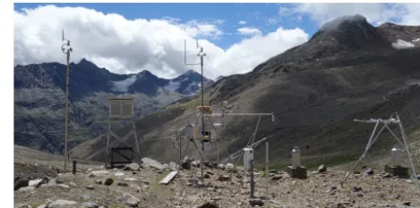
out at station “Hintereisferner” (3026 m a.s.l., 46.79867◦N, 10.76042◦E) (Fig. 10). The installation as of 2017 is detailed in Table 2.
Since 2014 an AWS has been seasonally operated on the glacier terminus, providing the meteorological data for sur-face energy balance assessments of the ice sursur-face, comple-mented by surface height change observations with a sonic ranger.
Figure 10.The Hintereisferner AWS and research station in June 2013 (3026 m a.s.l., 46.79867◦N, 10.76042◦E), view to the north-east. Photo by Christian Wild.
For KWF, only the meteorological observations on the glacier from 1958 by Ambach and Hoinkes (1963) are docu-mented.
3.2.2 Vernagtferner
After the start of the glacier monitoring program by the Bavarian Academy of Sciences and Humanities, me-teorological observations were initiated at the glacier forefield with the installation of a precipitation gauge in 1970. With the completion of the gauging station “Ver-nagtbach” (2635 m a.s.l., 46.85675◦N, 10.82886◦E; see Sect. 3.3.2), additional meteorological parameters have been observed since 1974 at the Vernagtbach climate station close by (2640 m a.s.l., 46.85663◦N, 10.82857◦E) (https://doi.org/10.1594/PANGAEA.775113). In 1975 hourly measurements of air temperature, relative humidity, air pressure, wind speed and direction were started. The same instruments were installed at the station “Gletscher-mitte” (3078 m a.s.l.), situated on a rock outcrop in the western part of the glacier at 46.86894◦N, 10.80299◦E, where hourly meteorological observations were col-lected during the summer months from 1968 until 1987 (with a varying beginning and end from year to year). The observed parameters were air temperature, relative humidity, wind speed and direction, and precipitation (https://doi.org/10.1594/PANGAEA.832562). Radiation sensors were installed at Vernagtbach in 1976. However, especially during winter, data gaps frequently occurred. The situation was considerably improved by installation of a first digital data logger in 1984. Since then, all-year data records are available from the Vernagtbach station (Escher-Vetter and Siebers, 2013). The meteorological observations were revised in 2002 with the installation of a modern AWS (Fig. 11), and since then all data are automatically trans-ferred to the Bavarian Academy of Sciences and Humanities via GSM and a satellite network. In August 2010, the
Figure 11. The Vernagtbach AWS in July 2017 (2640 m a.s.l., 46.85663◦N, 10.82857◦E), view to the southeast. Photo by Lud-wig Braun.
Hydrographic Service of Tyrol extended the installation with a separate temperature sensor and an unheated Pluvio 2 pluviometer (2630 m a.s.l., 46.85667◦N, 10.82861◦E). Details about the most recent sensor configurations are given in Table 3.
On “Schwarzkögele” (3075 m a.s.l., 46.86575◦N, 10.83245◦E), a summit in the vicinity of VF, an autonomous climate station has been in operation since 1976 (Braun et al., 2013). Data recorded there comprise air temperature, relative humidity, global radiation, wind speed and direction as well as precipitation. After digitization these measure-ments will be made available in PANGAEA. Experimeasure-ments and special investigations in the catchment of VF are listed in Escher-Vetter and Siebers (2013); since 2003, the meteo-rological observations have been extended to the ice surface of the glacier itself. Whereas in the first years these data have gaps (mainly in winter), they are mostly continuous since 2011.
3.2.3 Rofental apart from the glaciers
U. Strasser et al.: The Rofental 161
Table 2.Weather and snow variables recorded by the sensors installed at the station Hintereisferner (3026 m a.s.l., 46.79867◦N, 10.76042◦E) in 2010, 2011 and 2012. Accuracy according to technical data sheets of the manufacturers. Original temporal resolution of the data records is 10 min.
Variable Sensor Period of operation Accuracy Unit Air temperature Vaisala HMP45AC Since October 2010–present ±0.13◦C ◦C Relative humidity Vaisala HMP45AC Since October 2010–present ±2 % RH for 0–90 % RH, %
±3 % RH for 90–100 % RH
Wind speed and direction Young Wind Monitor Since October 2010–present 0.5–1 m s−1;±3◦ m s−1and◦ Shortwave and longwave Kipp & Zonen CNR 4 Since October 2010–present ±10 % (outgoing) W m−2 radiative fluxes <10 % (incoming)
Atmospheric pressure Setra CS 100 Since October 2010–present ±0.1 hPa hPa Soil and snow temperature BetaTherm 100K6A Since October 2010–present ±0.3◦C ◦C Snow depth Campbell SR50A Since October 2010–present 1 cm (or 0.4 % of distance) cm
Data 2010: https://doi.org/10.1594/PANGAEA.809091; 2011: https://doi.org/10.1594/PANGAEA.809094; 2012: https://doi.org/10.1594/PANGAEA.809095.
Table 3.Sensors and sampling intervals of the AWS Vernagtbach (2640 m a.s.l., 46.85663◦N, 10.82857◦E)∗.
Variable Sensor Period of operation Interval Unit Air temperature (ventilated) Thies PT-100 Since 2002 5 s 10 min−1 ◦C Air temperature (unventilated) PT-100 Since 2002 5 s 10 min−1 ◦C Relative humidity Thies hair hygrometer Since 2002 20 s 10 min−1 % Wind speed Thies cup anemometer Since 2002 5 s 10 min−1 m s−1 Wind direction Thies wind vane Since 2002 5 s 10 min−1 ◦ Shortwave downward radiation Kipp & Zonen CM7B unventilated Since 2002 5 s 10 min−1 W m−2 Shortwave upward radiation Kipp & Zonen CM7B unventilated Since 2002 5 s 10 min−1 W m−2 Longwave downward radiation Schenk Pyradiometer 8111 unventilated Since 2002 (summer only) 5 s 10 min−1 W m−2 Longwave upward radiation Schenk Pyradiometer 8111 unventilated Since 2002 (summer only) 5 s 10 min−1 W m−2 Precipitation sum Belfort weighing gauge Since 2002 5 s 10 min−1 mm Precipitation difference Gertsch tipping bucket, unheated Since 2002 Sum in 10 min mm Air pressure Druck RPT 410 Since 2002 20 s 10 min−1 hPa Snow depth Campbell SR50 Since 2002 120 s 10 min−1 mm
∗Further technical details can be found in Escher-Vetter and Siebers (2012). The additional temperature and rainfall recordings of the Hydrographic Service of Tyrol have been
separately available since August 2010, visualized online at http://apps.tirol.gv.at/hydro/#/Niederschlag/?station=197075; data upon request.
of operation of these totalizing rain gauges are given in Ta-ble 4.
Meteorological observations have been made in close proximity to the village of Vent since 1934 (Lauffer, 1966; Siogas, 1977b). This long-term station provides a valu-able reference for shorter series of meteorological obser-vations and also the lower boundary conditions on the likely variation of meteorological variables with eleva-tion across the catchment. Data are available for 1935– 2011 at https://doi.org/10.1594/PANGAEA.806582, and for 2012–2016 at https://doi.org/10.1594/PANGAEA.876595. In September 2015 the weather station installation was up-dated and the position changed by a horizontal displace-ment of 102 m (new position: 1907 m a.s.l., 46.85745◦N, 10.91288◦E). The recordings of this station comprise the meteorological variables air temperature, relative humidity, wind speed and direction (since February 2016), and atmo-spheric pressure (since September 2016; same instruments
and specifications as for station Hintereisferner, Table 2). Precipitation is recorded with a heated Ott Pluvio 2 in mil-limeters per hour with an accuracy of 0.1 mm h−1.
Table 4.Totalizing rain gauges in the Rofental.
Station Altitude Lat. (◦N) Long. (◦E) Period of operation DOI (m a.s.l.)
Vent 1900 46.85766 10.91127 1905–present https://doi.org/10.1594/PANGAEA.876532 Hochjochhospiz 2360 46.82310 10.82616 1952–present https://doi.org/10.1594/PANGAEA.876525 Vernagtbrücke 2600 46.85461 10.82979 1965–present https://doi.org/10.1594/PANGAEA.876533 Proviantdepot 2737 46.82951 10.82407 1952–present https://doi.org/10.1594/PANGAEA.876527 Rofenberg 2827 46.80847 10.79344 1952–present https://doi.org/10.1594/PANGAEA.876528 Latschbloder 2910 46.80118 10.80561 1965–present https://doi.org/10.1594/PANGAEA.876526 Hintereis station 2964 46.79727 10.76096 1952–present https://doi.org/10.1594/PANGAEA.876523 Saykogel 2990 46.80491 10.83459 1963–1980 https://doi.org/10.1594/PANGAEA.876529 Schwarzkögele 3075 46.86575 10.83245 1963–March 1977 https://doi.org/10.1594/PANGAEA.876531 Guslar 2920 46.85060 10.81489 October 1964– https://doi.org/10.1594/PANGAEA.876522
September 1981
Samoar 2650 46.80708 10.87539 1966–1974 https://doi.org/10.1594/PANGAEA.876530 Hintereisalm 2900 46.81941 10.78842 1965–September 1987 https://doi.org/10.1594/PANGAEA.876524
2015 and 2016 (mean annual temperature −1.3, −1.5 and −2.2◦C (WXT520), and annual precipitation: 1590, 1311 and 1118 mm (Pluvio 2 unheated)).
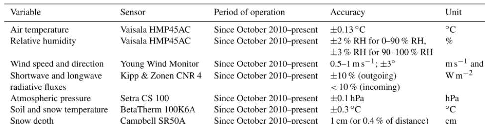
The weather station at Bella Vista includes a heated Ott Pluvio 2, supplied with main power from the “Schöne Aussicht-Hütte” approximately 90 m away. This site also in-cludes fuller snow instrumentation (Table 6) to measure: snow water equivalent (by means of a snow pillow), snow depth (by means of an ultrasonic ranger) and snow temper-ature profile (by means of a series of tempertemper-ature sensors at different height levels). These snow sensors are still un-dergoing technical examination and development, and as yet no check for consistency has been undertaken (e.g., by us-ing the data as input in a snow model as in Morin et al., 2012). In 2016, mean annual temperature at the station was −0.4◦C, and annual precipitation was 1605 mm. The Bella Vista weather and snow monitoring station is one of the high-est of its kind in the Alps. During summer 2017 an automatic camera that has the station in its field of view has been in-stalled (Fig. 12).
In summer 2017, a 6 m high tower close to the perma-nent terrestrial laser scanner on Im hintern Eis (3244 m a.s.l., 46.79586◦N, 10.78277◦E; see Sect. 3.4.2) was equipped for detailed turbulent flux measurements with the following sen-sors: three Lufft Ventus 2-D Sonic wind sensors at 1.5, 3 and 6 m altitude; two ventilated Rotronic HC2-S3 temperature– humidity sensors at 3 and 6 m altitude; a Campbell SR50 AH heated ultrasonic snow depth sensor in 1.5 m altitude; a Campbell Krypton hygrometer at 3 m altitude (only for spe-cific campaigns); a Kipp & Zonen CNR4 net radiometer at 1.5 m altitude; a Metek USA-1 3-D sonic turbulence sensor at 3 m altitude; and a Setra 278 barometric pressure sensor in the logger box. The data of these sensors will be made available in PANGAEA as soon as first tests have proven the installation to be reliable, and a time series of at least a year of data is available.
Figure 12. Webcam picture of the Bella Vista weather sta-tion (2805 m a.s.l., 46.78284◦N, 10.79138◦E), view to the East. Left: Ott Pluvio 2 with wind shelter. Center: temperature profiler. Right: snow pillow (foreground) and mast with sensors (back-ground) for wind speed and direction, snow height, tempera-ture/humidity and radiative fluxes. The most recent picture is avail-able at http://alpinehydroclimatology.net.
U. Strasser et al.: The Rofental 163
Table 5.Climate and snow variables recorded by the sensors installed at the station Latschbloder (2919 m a.s.l., 46.80106◦N, 10.80659◦E). Accuracy according to technical data sheets of the manufacturers. Original temporal resolution of the data records is 10 min.
Variable Sensor Period of operation Resolution and accuracy Unit Air temperature Vaisala WXT520 Since September 2013 0.1◦C±0.3◦C ◦C Relative humidity Vaisala WXT520 Since September 2013 0.1 %±3 % RH for 0–90 % RH, %
0.1 %±5 % RH for 90–100 % RH
Wind speed and Vaisala WXT520 Since September 2013 0.1 m s−1±3 % (speed) m s−1 direction 1◦±3 % for 10 m s−1(direction) and◦ Radiative fluxes Kipp & Zonen CNR 4 Since September 2013 10–20 W m−2(incoming) W m−2 (short- and longwave) 5–15 W m−2(outgoing)
Precipitation Vaisala WXT520 Since September 2013 0.01 mm h−1±5 %∗ mm Friedmann tipping bucket September 2013 to June 2014 (not yet known)
Ott Pluvio 2 v. 200 Since July 2014 0.01 mm h−1±1 % with wind shelter
Atmospheric pressure Vaisala WXT520 Since September 2013 0.1 hPa±0.5 hPa for 0–30◦C hPa 0.1 hPa±1.0 hPa for−52–60◦C
∗for hailstorm: 0.1 hit cm−2. The Vaisala WXT520 records rain and hail as well as their durations and intensities, but cannot recognize snowfall.
Data 2013: https://doi.org/10.1594/PANGAEA.879215; 2014: https://doi.org/10.1594/PANGAEA.879216; 2015: https://doi.org/10.1594/PANGAEA.879217; 2016: https://doi.org/10.1594/PANGAEA.879218; 2017: https://doi.org/10.1594/PANGAEA.879219.
Table 6.Weather and snow variables recorded by the sensors installed at the station Bella Vista (2805 m a.s.l., 46.78284◦N, 10.79138◦E). Accuracy according to technical data sheets of the manufacturers. Original temporal resolution of the data records is 10 min.
Variable Sensor Period of operation Resolution and accuracy Unit Air temperature E+E EE08 Since July, 2015 <0.5◦C1 ◦C
Vaisala WXT520 0.1◦C±0.3◦C
Relative humidity E+E EE08 Since July, 2015 ±2 % RH for 0–90 % RH, % Vaisala WXT520 ±3 % RH for 90–100 % RH
0.1 %±3 % RH for 0–90 % RH, 0.1 %±5 % RH for 90–100 % RH
Wind speed and direction Vaisala WXT520 Since July 2015 0.1 m s−1±3 % (speed) m s−1and◦ Kroneis 262 1◦±3 % for 10 m s−1(direction)
Radiative fluxes Kipp & Zonen CNR 4 Since July 2015 10–20 W m−2(incoming) W m−2 5–15 W m−2(outgoing)
Precipitation Vaisala WXT520 Since July 2015 0.01 mm h−1±5 %2 mm Ott Pluvio 2 v. 200 Since July, 2015 0.01 mm h−1±1 %
with wind shelter
Atmospheric pressure Vaisala WXT520 Since July, 2015 0.1 hPa±0.5 hPa for 0–30◦C hPa 0.1 hPa±1.0 hPa for−52–60◦C Snow water equivalent Sommer snow pillow 3×3 (still experimental)3 (still experimental) mm Snow depth Sommer USH-8 (still experimental)3 1 mm±0.1 % mm Snow temperature Pilz temperature profiler (still experimental)3 (still experimental) ◦C
1depending on air temperature; see technical data sheet of the manufacturer.2for hailstorm: 0.1 hit cm−2. The Vaisala WXT520 records rain and hail as well as their durations and intensities, but cannot recognize snowfall.3data not yet downloadable from PANGAEA. Data 2015: https://doi.org/10.1594/PANGAEA.879210; 2016:
3.3 Hydrological data
3.3.1 Hintereisferner and Kesselwandferner catchment
During the International Geophysical years 1957 to 1959 a gauging station was in operation at “Steg Hospiz” (2287 m a.s.l.), registering the combined streamflow from HEF and KWF (Lang, 1966). The measurements of this campaign are described here as an example for the many short- and longer-term monitoring activities carried out in the Rofental. The Steg Hospiz catchment is 26.6 km2in size, with a fraction of 58 % being covered by the glaciers at that time. Mean annual recorded streamflow for the catch-ment area amounted to 1848 mm (1957–1958) and 1770 mm (1958–1959), respectively (millimeters are equivalent to liters per square meter per year). Winter runoff (October through March) only was 5 and 10 % of the annual amount, whereas the three summer months (July through September) provided 76 and 72 %. Highest mean monthly streamflow amounts were registered in August 1958 (575 mm) and July 1959 (559 mm). The frequency distribution of daily stream-flow for 1957–1958 shows a period of daily low stream-flows of less than 0.5 m3s−1 (18.8 L s−1km−2) for 217 days (Oc-tober through May). Higher daily streamflow >6.0 m3s−1 (225 L s−1km−2) only occurred during July and August. The observed maximum daily streamflow was 16.9 m3s−1. The glacier contribution, determined as the fraction of (observed) negative mass balance to recorded streamflow, was relatively high in this period: 24 and 20 % of annual streamflow, respec-tively. The exponential decrease of the hydrograph in fall to the minimum in spring suggests that the winter streamflow mainly originates as delayed meltwater of the previous sea-son from the glaciers. The increase in the water flows after the beginning of the snow melt period occurs with a certain time delay – due to the refreezing of meltwater, and its reten-tion in the snow cover (Lang, 1966).
As of 2017, neither HEF nor KWF are equipped with a permanently registering discharge gauge; this is projected for future initiatives.
3.3.2 Vernagtferner catchment
The VF catchment is one of the very few glacierized catch-ments where simultaneous measurecatch-ments of glacier mass balance and discharge exist for several decades since 1974 (Escher-Vetter and Reinwarth, 2013). Discharge is measured at the gauge Vernagtbach (46.85675◦N, 10.82886◦E), which at 2635 m a.s.l. is the highest streamflow gauge in Austria (Fig. 13). The water level is continuously monitored in the gauge since 1974, and water-level-to-discharge calibrations are regularly conducted by the salt injection method. The water level is simultaneously determined by three sonic rangers distributed across the runoff channel in order to detect the 2-D surface geometry of the water flow, and surface velocity is monitored by a Doppler system. The total catchment area covers 11.44 km2, 7.3 km2 of
Figure 13.The Vernagtbach gauging station in 2006 (2635 m a.s.l., 46.85675◦N, 10.82886◦E), view to the northwest. Photo by Lud-wig Braun.
which was glacierized in 2015 (63.8 %). The vertical extent ranges from 2635 m a.s.l. at the gauge to 3635 m a.s.l. at the summit of “Hinterer Brochkogel” (see also Fig. 4). The discharge values are available as 5 min values for 2002 to 2012 (https://doi.org/10.1594/PANGAEA.829530). Hourly hydrological records for the Vernagtbach catchment are available for the period 1974 to 2001 at https://doi.org/10.1594/PANGAEA.775113. Monthly averages of discharge are available at https://doi.org/10.1594/PANGAEA.832432, and yearly values are available for the period 1974 to 2012 at https://doi.org/10.1594/PANGAEA.832429.
3.3.3 Rofental catchment
U. Strasser et al.: The Rofental 165
Figure 14.The rainfall totalisator and the gauge at Vent (1891 m a.s.l., 46.85722◦N, 10.91083◦E) (a; Photo: Hydrographic Service of the Tyrol), and mean monthly streamflow of the Rofenache 1971–2009(b). Data from the Hydrographisches Jahrbuch (BMLFUW 2011).
3.4 Laser scanning data
Laser scanning is an active remote sensing technique which uses a laser beam to acquire 3-D point data, representing the surface and objects on that surface in high spatial resolution. In addition to high accuracy and resolution, additional infor-mation on the spectral properties intensity and reflectance of the scanned surface in the wavelength of the specific scanner is recorded. The DTMs derived from laser scanning measure-ments are becoming increasingly important for glaciological and geomorphological studies. DTM differencing is an im-portant method for detection and quantification of surface changes and mass budget calculations (Sailer et al., 2014; Klug et al., 2017). Airborne laser scanning (ALS) and ter-restrial laser scanning (TLS) are the most common methods for lidar data collection (Telling et al., 2017). The Rofental has been an intensive experimental site for both types of laser scanning data processing and analysis.
3.4.1 Airborne laser scans
ALS is well-suited for remote mountain areas, because no ex-ternal light source is required and, due to overlapping flight strips, the entire surface is captured, even in very steep ter-rain (Höfle and Rutzinger, 2011). The vertical accuracy is in the order of 0.05 to 0.20 m, mainly dependent on the slope angle (Beraldin et al., 2010; Bollmann et al., 2011). Low vertical errors of 0.05 m were observed in the HEF catch-ment for areas with slope angle<40◦by comparison of an ALS-derived DTM with dGNSS (differential global naviga-tion satellite system) measurements. For the areas with slope angle>40◦, an exponential increase of the vertical error was observed (1.0 m for 80◦, Bollmann et al., 2011; Geist et al., 2005; Sailer et al., 2012).
The HEF data set is built from 21 separate ALS acqui-sitions from 2001 to 2013, covering an area of 32 km2, including HEF (approx. 6.8 km2 in 2011), KWF (approx. 3.8 km2in 2011), “Langtaufererjochferner” (approx. 1.1 km2 in 2011) and “Stationsferner” (approx. 0.3 km2 in 2011).
DEMs of 1×1 m were generated by calculating thezvalue (altitude) from the meanz value inside the respective grid cell by excluding 5 % of the smallest and largest observa-tions of the ALS points. For the provision of the GeoTIFF (UTM32N) raster files the high-resolution DEMs were re-sampled to DEMs with a cell size of 10×10 m, applying bilinear interpolation. The resulting DEMs are available at https://doi.org/10.1594/PANGAEA.875889.
The available ALS measurements for HEF were used to study the volume changes of the glacier complementary to direct glaciological surface mass balance measurements. At least one scan was performed at the end of every glacier mass balance year (end of September). From these, a time series of geodetic mass balances was derived for 2001–2002 to 2010–2011 (see Fig. 8). In 2001–2002, 2002–2003, 2007– 2008, 2008–2009 and 2010–2011 additional project-based intermediate campaigns were carried out. An overview of the data (UTM32N, WGS84) including the technical details is given in Table 7. Klug et al. (2017) corrected the surface models as well as glacier mass balance data by considering method-inherent uncertainties originating from snow cover, survey dates and density assumptions to calculate corrected annual geodetic mass balances. The most negative balance year is 2002–2003, with a mean specific mass balance of −2.713±0.20 m water equivalent (w.e.). In the subsequent mass balance year 2003–2004, the smallest mass loss is ob-served (mean specific mass balance−0.654±0.09 m w.e.). For the entire observation period (2001 to 2011) a mean mass balance of −1.3 m w.e. was calculated with the HEF ALS data set (Klug et al., 2017).
Table 7.Overview of the available HEF ALS data with flight date, used Optech sensor, mean flight height above ground (m), maximum scanning angle (◦), pulse repetition rate (Hz), across-track overlap (%), mean point density (points m−2) and vertical accuracy (m). Data are available at https://doi.org/10.1594/PANGAEA.875889.
Mean Maximum Pulse Mean Vertical Flight date Optech height above scanning repetition Across-track point density accuracy Sensor ground (m) angle (◦) rate (Hz) overlap (%) (points m−2) (m) 11 Oct 2001 ALTM 1225 900 20 25 000 24 1.1 0.11 9 Jan 2002 ALTM 1225 900 20 25 000 24 1.2 0.14 7 May 2002 ALTM 1225 900 20 25 000 24 1.2 0.14 15 Jun 2002 ALTM 1225 900 20 25 000 24 1.3 0.14 8 Jul 2002 ALTM 1225 900 20 25 000 24 1.4 0.15 19 Aug 2002 ALTM 1225 900 20 25 000 24 1.4 0.10 18 Sep 2002 ALTM 3033 900 20 33 000 24 1.0 0.10 4 May 2003 ALTM 2050 1150 20 50 000 40 0.8 0.10 12 Aug 2003 ALTM 2050 1150 20 50 000 40 0.8 0.10 26 Sep 2003 ALTM 1225 900 20 25 000 24 1.0 0.06 5 Oct 2004 ALTM 2050 1000 20 50 000 24 2.0 0.07 12 Oct 2005 ALTM 3100 1000 22 70 000 50–70 3.4 0.07 8 Oct 2006 ALTM 3100 1000 20 70 000 37–75 2.0 0.08 11 Oct 2007 ALTM 3100 1000 20 70 000 37–75 3.4 0.06 9 Sep 2008 ALTM 3100 1000 20 70 000 40-45 2.2 0.06
7 May 2009 ALTM 3100 – – – – – –
30 Sep 2009 ALTM 3100 1100 20 70 000 31–66 2.7 0.05 8 Oct 2010 ALTM Gemini 1000 25 70 000 62 3.6 0.03 4 Oct 2011 ALTM 3100 1100 20 70 000 25–75 2.9 0.04 11 May 2012 ALTM 3100 1200 20 70 000 31–66 2.8 0.06 3 Sep 2013 ALTM Gemini 1200 20 70 000 59–80 4.2 0.04
3.4.2 Terrestrial laser scans – the permanent laser scanner on Im hintern Eis
The utility of TLS in performing high-resolution glacier ob-servations was tested for HJF from 2013–2015 when both glaciological and geodetic mass balances were measured. Likewise, a Riegl VZ-6000 TLS was used to produce sur-face models within 0.1 m of coincident high-accuracy ALS data for approx. 80 % of the surface of HJF. The TLS surface models are of higher spatial resolution and surface details than the ALS. The TLS data were used – along with coinci-dent optical imagery from the onboard camera – to produce high-resolution surface classifications to map snow-cover ex-tent, and to explore the spatial patterns of the surface mass balance of HJF (Prantl et al., 2017).
In 2016, a permanent TLS was installed in a climate con-trolled container at 3244 m a.s.l. close to the summit Im hin-tern Eis (46.79586◦N, 10.78277◦E). The 3-D laser scanner VZ-6000 (manufactured by RIEGL Laser Measurement Sys-tems GmbH) offers a long measurement range of more than 6000 m and operates with beam divergence of 0.12 mrad at a wavelength of 1050 nm, particularly suited for snow- and ice-related applications. The device operates with an angu-lar step width of 0.01◦ for a field of view of 60◦ verti-cally and 120◦horizontally and a laser pulse repetition rate of 30 kHz, equivalent to an effective measurement rate of
23 000 measurements s−1, leading to a point density of ap-prox. 10 pts m−2for a distance of 1000 m, and to approx. 1 to 2 pts m−2for the remote areas at a distance of>3500 m. Hence, the instrument is ideal for static topographic appli-cations such as monitoring of glaciological and geomorpho-logical processes in high mountain terrain. Due to the large field of view, nearly the entire HEF catchment area can be covered by the instrument (Fig. 15); only a very small part of the terminus and small flat areas in the upper glacier zones cannot be sampled. The TLS surface point cloud is accom-panied by high-quality optical imagery (5 megapixel). This installation not only allows high temporal and spatial reso-lution glacier volume changes for HEF to be determined; in addition, the high spatial resolution supports the monitoring of surface features such as crevasses, evolving surface rough-ness, the supraglacial drainage network and geomorpho-dynamically induced surface changes (e.g., debris flows) or snow avalanches. Seven scans have been carried out during the test phase (September 2016 to April 2017).
4 Data availability
ac-U. Strasser et al.: The Rofental 167
Figure 15.The terrestrial laser scanner in its container housing at Im hintern Eis (3244 m a.s.l., 46.79586◦N, 10.78277◦E). View to the west over the upper areas of Hintereisferner to the summit of Weisskugel (3739 m a.s.l.) and Langtauferer Spitze (3529 m a.s.l.). Photo by Rudolf Sailer.
tivities. These data sets, however, represent only a small fraction of what has been observed and collected during the past few decades. Many measurements have been con-ducted during special field campaigns and are not yet docu-mented for online data publication. For example, hydrolog-ical investigations have been conducted in the valley of the Hochjochbach, including streamflow observations with pres-sure sensors and tracer experiments since 2014 (Schmieder et al., 2016, 2018). Other data await digitization and pro-cessing. Originally published in analogue printwork, these data include 3 years of hourly ice temperatures from HEF (Markl and Wagner, 1978), observations of sublimation of ice and snow at HEF (Kaser, 1982, 1983), firn investiga-tions at KWF (Ambach et al., 1978), remote sensing ex-periments and many energy balance investigations at HEF (Jaffé, 1958, 1960; Hoinkes and Untersteiner, 1952; Hoinkes, 1953a, b; Ambach and Hoinkes, 1963; Wendler, 1967; Kuhn et al., 1979, Wagner, 1979, 1980), and many others. For VF, the situation is similar; a comprehensive overview of the research work has been published by Braun and Escher-Vetter (2013), including various descriptions and documen-tations of the used data, methods and models. Older long-term field experiments at VF are described in Moser et al. (1986). Runoff data of the gauge “Vent” have been widely used in hydrological studies, the most recent ones includ-ing Schmieder et al. (2016) and Hanzer et al. (2016, 2017). On a regional scale, the Rofental data contributed to mod-eling exercises for future scenario climatic conditions and their effect on simulated streamflow discharge (Marke et al., 2011, 2013). The Hydrographic Service of Tyrol visualizes its data online at apps.tirol.gv.at/hydro, and provides their download at http://ehyd.gv.at. As of 2017, data of the sites
Latschbloder and Schöne Aussicht are used in several ongo-ing research projects (listed at http://alpinehydroclimatology. net), and also provide valuable experimental material for ap-plication in various student courses.
Several initiatives are also ongoing at the international research network level. Apart from its long history within UNESCO IHP (http://en.unesco.org/themes/water-security/ hydrology), the Rofental recently became a research basin in the framework of the GEWEX INARCH project (http:// words.usask.ca/inarch). It is a research catchment of the ERB Euro-Mediterranean Network of Experimental and Repre-sentative Basins (http://erb-network.simdif.com), and a reg-ular complex site in the LTSER platform Tyrolean Alps (http://lter-austria.at/ta-tyrolean-alps), which belongs to the national and international long term ecological research net-work (LTER Austria, LTER Europe and ILTER). Hintereis-ferner station is part of the EU Horizon 2020 INTERACT framework of Arctic (and a few Alpine) research stations (https://eu-interact.org/field-sites/station-hintereis/).
The efforts to provide the Rofental data to the scientific community will continue in all of the currently involved in-stitutions.
5 Conclusions and outlook
The Rofental in the Ötztal Alps (Austria) is a unique, high Alpine research basin (98.1 km2, 1890–3770 m a.s.l.) with available time series of 150 years of glaciological and hy-drometeorological observations. The glaciers in the Rofental attracted early attention and were – for centuries – observed due to the dangerous nature of frequently occurring glacier lake outburst floods. Over the last 100 years, the glacier mon-itoring has been accompanied by systematic recordings of meteorological and hydrological variables. Today, a glacio-logical and hydrometeoroglacio-logical data set is available for the Rofental that is without comparison worldwide, with re-gard to both its amount and temporal coverage. The Rofen-tal data sets support manifold investigations in the context of coupled climate and glacier evolution, snow and glacier hydrology, water resources availability in mountainous re-gions, or method development like laser scanning or mod-eling. The scales of such research range from local, like particular micrometeorological assessments at a single ob-servation site, to global, e.g., the estimation of the glacier contribution to sea level rise. This paper gives an overview of what has been measured and what is available already. All the data described are comprehensively documented and made freely available according to the Creative Commons Attribution License by means of the PANGAEA repository (https://doi.org/10.1594/PANGAEA.876120).
will add to the extension of the records back in time (left side of the bars in Fig. 6). New and future data will continue to further build on the available Rofental database (right side of the bars in Fig. 6). This process of continuous enlargement of the data described here is ensured by the living data process as conceived by the journal.
Competing interests. The authors declare that they have no con-flict of interest.
Special issue statement. This article is part of the special is-sue “Hydrometeorological data from mountain and alpine research catchments”. It is not associated with a conference.
Acknowledgements. Many of the instruments and the monitor-ing activities presented here have been supported by the institu-tions to which the authors are affiliated to, and by countless re-search programs. These have been funded by the Bavarian Academy of Sciences and Humanities (BAdW), the Deutsche Forschungs-gemeinschaft (DFG), the Austrian Academy of Sciences (ÖAW; project HydroGeM3), the European Region Tyrol – South Tyrol – Trentino (project CRYOMON-SciPro – IPN 10-N33), the Au-tonomous Province of Bolzano – South Tyrol (project hiSnow – 23/40.3), the Austrian Federal Ministry of Agriculture, Forestry, Environment and Water Management (BMLFUW, section IV/4-water cycle), and others. The laser data acquisition and processing has been funded by the European Union (project OMEGA – EVK2-CT-2000-00069), the Austrian Research Promotion Agency FFG ASAP (Austrian Space Applications Programme; projects ALS-X – 815527 and SE.MAP – 840109), the Austrian Research Pro-motion Agency FFG COMET (Competence Centers for Excellent Technologies) in cooperation with the alpS GmbH (project MU-SICALS – 826388), the Austrian Climate Research Programme (ACRP; project C4AUSTRIA – A963633), the Tyrolean Science Foundation (TWF) and the Department of Geography, University of Innsbruck.
All these funding institutions provide the support to continue our efforts in the monitoring of the water balance and climate elements of the Rofental in the long term. The authors gratefully acknowledge all the contributions and support from their countless colleagues in maintaining the instruments in the field, being so many that they cannot be listed here by name. Without their engagement, the long-term monitoring in the Rofental would never have been possible.
Edited by: Danny Marks
Reviewed by: Stefan Pohl, Samuel Morin, Patrick Kormos, and Adam Winstral
References
Abermann, J., Lambrecht, A., Fischer, A., and Kuhn, M.: Quanti-fying changes and trends in glacier area and volume in the Aus-trian Ötztal Alps (1969–1997–2006), The Cryosphere, 3, 205– 215, https://doi.org/10.5194/tc-3-205-2009, 2009.
Ambach, W. and Hoinkes, H. C.: The heat balance of an Alpine snow field (Kesselwandferner, 3240 m, Oetztal Alps, 1958), IAHS Publ., 61, 24–36, 1963.
Ambach, W., Blumenthaler, M., Eisner, H., Kirchlechner, P., Schneider, H., Behrens, H., Moser, H., Oerter, H., Rauert, W., and Bergmann, H.: Untersuchungen der Wassertafel am Kessel-wandferner (Ötztaler Alpen) an einem 30 Meter tiefen Firn-schacht, Z. Gletscherkd. Glazialgeol., 14, 61–71, 1978. Beraldin, J.-A., Blais, F., and Lohr U.: Laser scanning technology,
in: Airborne and Terrestrial Laser Scanning, edited by: Vossel-man, G. and Maas, H.-G., Whittles Publishing, Dunbeath, UK, 1–42, 2010.
Blümcke, A. and Hess, H.: Der Hochjochferner im Jahre 1883, Zeitschrift des Deutschen und Österreichischen Alpenvereins, Verlag des D. u. Ö. AV, München, 26 pp., 1895.
Blümcke, A. and Hess, H.: Untersuchungen am Hintereis-ferner, Wissenschaftliche Ergänzungshefte zur Zeitschrift des Deutschen und Österreichischen Alpenvereins, Verlag des D. u. Ö. AV, München, 87 pp., 1899.
BMLFUW: Hydrographisches Jahrbuch von Österreich 2009, Bun-desministerium für Land- und Forstwirtschaft, Umwelt und Wasserwirtschaft, Wien, 2011.
Bollmann, E., Sailer, R., Briese, C., Stötter, J., and Fritzmann, P.: Potential of airborne laser scanning for geomorphologic feature and process detection and quantifications in high alpine moun-tains, Z. Geomorph., 55, 83–104, 2011.
Braun, L. and Escher-Vetter, H. (Eds.): Gletscherforschung am Vernagtferner, Themenband zum fünfzigjährigen Gründungsju-biläum der Kommission für Glaziologie der Bayerischen Akademie der Wissenschaften München, Z. Gletscherkd. Glazialgeol., 45/46, 389 pp., 2013.
Braun, L., Reinwarth, O., and Weber, M.: Der Vernagtferner als Ob-jekt der Gletscherforschung, Z. Gletscherkd. Glazialgeol., 45/46, 85–104, 2013.
Brunner, K.: Karten und Ansichten des Vernagtferners seit 1600, Z. Gletscherkd. Glazialgeol., 45/46, 235–257, 2013.
Charalampidis, C., Braun, L., Fischer, A., Kuhn, M., Lambrecht, A., Mayer, C., Thomaidis, K. and Weber, M.: Effect of glacier geometry on mass loss in a warming climate, J. Geophys. Res.-Earth, in review, 2018.
Cogley, J. G., Hock, R., Rasmussen, L. A., Arendt, A. A., Bauder, A., Braithwaite, R. J., Jansson, P., Kaser, G., Müller, M., Nichol-son, L., and Zemp, M.: Glossary of Glacier Mass Balance and Related Terms, IHP-VII Technical Documents in Hydrology No. 86, IACS Contribution No. 2, UNESCO-IHP, Paris, 2011. Escher-Vetter, H. and Oerter, H.: Das Energiebilanz- und
Abflussmodel PEV – frühe Modellansätze, Erweiterungen und ausgewählte Ergebnisse, Z. Gletscherkd. Glazialgeol., 45/46, 129–142, 2013.
Escher-Vetter, H. and Reinwarth, O.: Meteorologische und hydrolo-gische Registrierungen an der Pegelstation Vernagtbach – Chara-teristika und Trends ausgewählter Parameter, Z. Gletscherkd. Glazialgeol., 45/46, 117–128, 2013.
Escher-Vetter, H. and Siebers, M.: Technical comments on the data records from the Vernagtbach station for the period 2002 to 2012, Commission for Geodesy and Glaciology, Section Glaciology Bavarian Academy of Sciences and Humanities, Munich, 2012. Escher-Vetter, H. and Siebers, M.: Vom Registrierstreifen zur
Aufzeich-U. Strasser et al.: The Rofental 169
nungsgeräte an der Pegelstation Vernagtbach, Z. Gletscherkd. Glazialgeol., 45/46, 105–116, 2013.
Finsterwalder, S.: Der Vernagtferner, seine Geschichte und seine Vermessung in den Jahren 1888 und 1898, Wissenschaftliche Ergänzungshefte zur Zeitschrift des Deutschen und Österreichis-chen Alpenvereins, Verlag des D. u. Ö. AV, Graz, 112 pp., 1897. Fischer, A., Seiser, B., Stocker Waldhuber, M., Mitterer, C., and Abermann, J.: Tracing glacier changes in Austria from the Lit-tle Ice Age to the present using a lidar-based high-resolution glacier inventory in Austria, The Cryosphere, 9, 753–766, https://doi.org/10.5194/tc-9-753-2015, 2015.
Geist, T. and Stötter, J.: First results on airborne laser scanning technology as a tool for the quantification of glacier mass bal-ance, Proceedings of EARSeL-LISSIG-Workshop Observing our Cryosphere from Space, Bern, Switzerland, 11–13 March 2002. Geist, T., Elvehøy, H., and Jackson, M.: Investigations on
intra-annual elevation changes using multi-temporal airborne laser scanning data: case study Engabreen, Norway, Ann. Glaciol. 42, 195–201, https://doi.org/10.3189/172756405781812592, 2005. Hanzer, F., Helfricht, K., Marke, T., and Strasser, U.: Multilevel
spa-tiotemporal validation of snow/ice mass balance and runoff mod-eling in glacierized catchments, The Cryosphere, 10, 1859–1881, https://doi.org/10.5194/tc-10-1859-2016, 2016.
Hanzer, F., Förster, K., Nemec, J., and Strasser, U.: Projected cryospheric and hydrological impacts of 21st century cli-mate change in the Ötztal Alps (Austria) simulated using a physically based approach, Hydrol. Earth Syst. Sci. Discuss., https://doi.org/10.5194/hess-2017-309, in review, 2017. Harding, R. J., Entrasser, N., Escher-Vetter, H., Jenkins, A., Kaser,
M., Kuhn, M., Morris, E. M., and Tanzer, G.: Energy and mass balance studies in the firn area of the Hintereisferner, in: Glacier fluctuations and climatic change, Glaciology and Quaternary Ge-ology, Kluwer, Dordrecht, 325–341, 1989.
Helfricht, K., Kuhn, M., Keuschnig, M., and Heilig, A.: Lidar snow cover studies on glaciers in the Ötztal Alps (Austria): com-parison with snow depths calculated from GPR measurements, The Cryosphere, 8, 41–57, https://doi.org/10.5194/tc-8-41-2014, 2014a.
Helfricht, K., Schöber, J., Schneider, K., Sailer, R., and Kuhn, M.: Interannual persistence of the seasonal snow cover in a glacierized catchment, J. Glaciol., 60, 889–904, https://doi.org/10.3189/2014JoG13J197, 2014b.
Hess, H.: Die Gletscher, Nabu Press, Braunschweig, 426 pp., 1904. Höfle, B. and Rutzinger, M.. Topographic airborne LiDAR in geomorphology: A technological perspective, Z. Geomorph., 55, 1–29, https://doi.org/10.1127/0372-8854/2011/0055S2-0043, 2011.
Hoinkes, H.: Zur Mikrometeorologie der eisnahen Luftschicht, Arch. Met. Geoph. Biokl., 4, 451–458, 1953a.
Hoinkes, H.: Wärmeumsatz und Ablation auf Alpengletschern: II – Hornkees (Zillertaler Alpen), Geogr. Ann., 35, 116–140, https://doi.org/10.1080/20014422.1953.11880853, 1953b. Hoinkes, H.: Methoden und Möglichkeiten von
Massen-haushaltsstudien auf Gletschern, Ergebnisse der Messreihe Hintereisferner (Ötztaler Alpen) 1953–1968, Z. Gletscherkd. Glazialgeol., 6, 37–90, 1970.
Hoinkes H. und Steinacker, R.: Zur Parametrisierung der Beziehung Klima – Gletscher, Rivista Italiana di Geofisica, I, 97–104, 1975.
Hoinkes, H. and Untersteiner, N.: Wärmeumsatz und Ablation auf Alpengletschern I, Vernagtferner (Ötztaler Alpen), August 1950, Geogr. Ann., 34, 99–158, 1952.
Hoinkes, H., Dreiseitl, E., and Wagner, H. P.: Mass Balance of Hin-tereisferner and Kesselwandferner 1963/64 to 1972/73 in Rela-tion to the Climatic Environment, Preliminary results of the corn-bined water, ice and heat balances project in the Rofental, IHD-Activities in Austria 1965–1974, Report of the Int. Conference on the Results of the IHD, Paris, 2–14 September 1974, 42–53, 1974.
Jaffé, A.: Neuere Albedo- und Extinktionsmessungen an Gletschereisplatten, Ber. Dt. Wetterdienstes, 54, 273–274, 1958.
Jaffé, A.: Über Strahlungseigenschaften des Gletschereises, Archiv Met. Geoph. Biokl., Edn. 10, 376–395, https://doi.org/10.1007/BF02243201, 1960.
Juen, M., Mayer, C., Lambrecht, A., Eder, K., Wirbel, A., and Stilla, U.: Einsatz einer Thermalkamera und von Strahlungssen-soren zur Oberflächenklassifizierung am Vernagtferner, Z. Gletscherkd. Glazialgeol., 45/46, 185–201, 2013.
Kaser, G.: Measurements of Evaporation from Snow, Archiv Met. Geoph. Biokl., Ser. B, 30, 333–340, 1982.
Kaser, G.: Über die Verdunstung auf dem Hintereisferner, Z. Gletscherk. Glazialgeol., 19, 149–162, 1983.
Kaser, G., Grosshauser, M., and Marzeion, B.: Contribution poten-tial of glaciers to water availability in different climate regimes, P. Natl. Acad. Sci. USA, 107, 20223–20227, 2010.
Klug, C., Rieg, L., Ott, P., Mössinger, M., Sailer, R., and Stöt-ter, J.: A Multi-Methodological Approach to Determine Per-mafrost Occurrence and Ground Surface Subsidence in Moun-tain Terrain, Tyrol, Austria, Permafrost Periglac., 28, 249–265, https://doi.org/10.1002/ppp.1896, 2016.
Klug, C., Bollmann, E., Galos, S. P., Nicholson, L., Prinz, R., Rieg, L., Sailer, R., Stötter, J., and Kaser, G.: A reanaly-sis of one decade of the mass balance series on Hintereis-ferner, Ötztal Alps, Austria: a detailed view into annual geode-tic and glaciological observations, The Cryosphere Discuss., https://doi.org/10.5194/tc-2017-132, in review, 2017.
Kreuss, O.: Compiled geological map of ÖK50 Sheet 173 – Sölden, preliminary GEOFAST 1 : 50 000 edition 2016/03, Geologische Bundesanstalt Wien Publishing House, 2012.
Kuhn, M.: Micro-meteorological conditions for snow melt, J. Glaciol., 33, 24–26, 1987.
Kuhn, M., Kaser, G., Markl, G., Wagner, H. P., and Schneider, H. (Eds.): 25 Jahre Massenhaushaltsuntersuchungen am Hintereis-ferner, Auszug aus den glazialmeteorologischen Arbeiten im Ge-biet des Hintereisferners in den Ötztaler Alpen, Institut für Mete-orologie und Geophysik der Universität Innsbruck, 80 pp., 1979. Kuhn, M., Kaser, G., Markl, G., Nickus, U., and Obleitner, F.: Fluc-tuations of Mass Balance and Climate: The 30 Years Record of Hintereis- and Kesselwandferner, Z. Gletscherkd. Glazialgeol., 22, 490–416, 1985a.
Kuhn, M., Markl, G., Kaser, G., Nickus, U., Obleitner, F., and Schneider, H.: Fluctuations of climate and mass balances: Differ-ent responses of two adjacDiffer-ent glaciers, Z. Gletscherkd. Glazial-geol., 21, 409–416, 1985b.
balance of Hintereisferner, Geogr. Ann. A, 81, 659–670, https://doi.org/10.1111/1468-0459.00094, 1999.
Kuhn, M., Abermann, J., Olefs, M., Fischer, A., and Lambrecht, A.: Gletscher im Klimawandel: Aktuelle Monitoring- programme und Forschungen zur Auswirkung auf den Gebietsabfluss im Ötztal, Mitt. hydr. Dienst Österr., 86, 31–47, 2006.
Kuhn, M., Lambrecht, A., Abermann, J., Patzelt, G., and Groß, G.: Die österreichischen Gletscher 1998 und 1969, Flächen- und Vol-umenänderungen, Verlag der österr. Akad. Wiss., Wien, available at: hw.oeaw.ac.at/6616-0, 128 pp., 2009.
Kuhn, M., Lambrecht, A., Abermann, J., Patzelt, G., and Groß, G.: The Austrian Glaciers 1998 and 1969, Area and Volume Changes, Z. Gletscherkd. Glazialgeol., 43/44, 3–107, 2012. Lambrecht, A. and Kuhn, M.: Glacier changes in the
Aus-trian Alps during the last three decades, derived from the new Austrian glacier inventory, Ann. Glaciol., 46, 177–184, https://doi.org/10.3189/172756407782871341, 2007.
Lang, H.: Hydrometeorologische Ergebnisse aus Abflußmessungen im Bereich des Hintereisferners (Ötztaler Alpen) in den Jahren 1957–1959, Archiv Met. Geoph. Biokl. B, 14, 280–302, 1966. Lauffer, I.: Das Klima von Vent, Dissertation, University of
Innsbruck, available at: http://acinn.uibk.ac.at/sites/default/files/ Diss_Lauffer_Ingrid_1966.pdf, 1966.
Lindmayer, A.: Untersuchung zum Einfluss der Veränderung der Topographie der Eisoberfläche auf die spezifische Massen-bilanz eines Gletschers am Beispiel des Vernagtferners im Zeitraum 1889–1938, Master Thesis, Catholic University of Eichstätt-Ingolstadt, Faculty of Mathematics and Geography, 102 pp., available at: http://kegglaziologie.de/download/MSc_ A_Lindmayer2015.pdf (last access: 26 November 2017), 2015. Marke, T., Mauser, W., Pfeiffer, A., and Zängl, G.: A
prag-matic approach for the downscaling and bias correction of re-gional climate simulations: evaluation in hydrological modeling, Geosci. Model Dev., 4, 759–770, https://doi.org/10.5194/gmd-4-759-2011, 2011.
Marke, T., Mauser, W., Pfeiffer, A., Zängl, G., Jacob, D., and Strasser, U.: Application of a hydrometeorological model chain to investigate the effect of global boundaries and downscaling on simulated river discharge, Environ. Earth Sci., 71/11, 4849– 4846, https://doi.org/10.1007/s12665-013-2876-z, 2013. Markl, G. and Wagner, H. P.: Messungen von Eis- und
Firntemper-aturen am Hintereisferner (Ötztaler Alpen), Symposium über die Dynamik temperierter Gletscher, Z. Gletscherkd. Glazialgeol., 13, 261–265, 1978.
Marzeion, B. and Levermann, A.: Loss of cultural world heritage and currently inhabited places to sea-level rise, Environ. Res. Lett., 9, 051001, https://doi.org/10.1088/1748-9326/9/3/034001, 2014.
Marzeion, B. and Kaser, G.: Peak Water: An Unsustainable Increase in Water Availability From Melting Glaciers, Mountains and cli-mate change: A global concern, Centre for Development and En-vironment (CDE), Swiss Agency for Development and Coopera-tion (SDC) and Geographica Bernensia, Bern, 47–50, 2014. Marzeion, B., Jarosch, A. H., and Hofer, M.: Past and future
sea-level change from the surface mass balance of glaciers, The Cryosphere, 6, 1295–1322, https://doi.org/10.5194/tc-6-1295-2012, 2012a.
Marzeion, B., Hofer, M., Jarosch, A. H., Kaser, G., and Mölg, T.: A minimal model for reconstructing interannual mass balance
variability of glaciers in the European Alps, The Cryosphere, 6, 71–84, https://doi.org/10.5194/tc-6-71-2012, 2012b.
Marzeion, B., Cogley, J. G., Richter, K., and Parkes, D.: Attribution of global glacier mass loss to anthro-pogenic and natural causes, Science, 345, 919–921, https://doi.org/10.1126/science.1254702, 2014a.
Marzeion, B., Jarosch, A. H., and Gregory, J. M.: Feedbacks and mechanisms affecting the global sensitivity of glaciers to climate change, The Cryosphere, 8, 59–71, https://doi.org/10.5194/tc-8-59-2014, 2014b.
Mayer, C., Escher-Vetter, H., and Weber, M.: 46 Jahre glaziologis-che Massenbilanz des Vernagtferners, Z. Gletsglaziologis-cherkd. Glazial-geol., 45/46, 219–234, 2013a.
Mayer, C., Lambrecht, A., Blumthaler, U., and Eisen, O.: Ver-messung und Eisdynamik des Vernagtferners, Ötztaler Alpen, Z. Gletscherkd. Glazialgeol., 45/46, 259–280, 2013b.
Morin, S., Lejeune, Y., Lesaffre, B., Panel, J.-M., Poncet, D., David, P., and Sudul, M.: An 18-yr long (1993–2011) snow and meteo-rological dataset from a mid-altitude mountain site (Col de Porte, France, 1325 m alt.) for driving and evaluating snowpack mod-els, Earth Syst. Sci. Data, 4, 13–21, https://doi.org/10.5194/essd-4-13-2012, 2012.
Moser, H., Escher-Vetter, H., Oerter, H., Reinwarth, O., and Zunke, D.: Abfluß in und von Gletschern, Technical University of Mu-nich (TUM), Special Research Report 81, Final Report Project A1, GSF-Bericht, 41/86, 1–397, 1986.
Moser, M.: Compiled geological map of ÖK50 Sheet 172 – Weißkugel, preliminary GEOFAST 1 : 50 000 edition 2016/03, Geologische Bundesanstalt Wien, Publishing House, 2012. Müller, G., Godina, R., and Gattermayer, W.: Der Pegel
Vent/Rofenache – Herausforderungen für eine hydrographische Messstelle in einem vergletscherten Einzugsgebiet, Mitt. hydr. Dienst Österr., 86, 131–135, 2009.
Nicolussi, K.: Bilddokumente zur Geschichte des Vernagtferners im 17. Jahrhundert, Z. Gletscherkd. Glazialgeol., 26, 97–119, 1990. Nicolussi, K.: Die historischen Vorstöße und Hochstände des
Ver-nagtferners, Z. Gletscherkd. Glazialgeol., 45/46, 9–23, 2013. Obleitner, F.: Climatological features of glacier and valley winds at
the Hintereisferner (Ötztal Alps, Austria), Theor. Appl. Clima-tol., 49, 225–239, 1994.
Painter, T. H., Flanner, M. G., Kaser, G., Marzeion, B., VanCuren, R. A., and Abdalati, W.: End of the Little Ice Age in the Alps forced by industrial black carbon, P. Natl. Acad. Sci. USA, 110, 15216–15221, https://doi.org/10.1073/pnas.1302570110, 2013. Prantl, H., Nicholson, L., Sailer, R., Hanzer, F., Juen, I.,
and Rastner, P.: Glacier snowline determination from ter-restrial laser scanning intensity data, Geosciences, 7, 1–21, https://doi.org/10.3390/geosciences7030060, 2017.
Prasch, M., Marke, T., Strasser, U., and Mauser, W.: Large scale in-tegrated hydrological modelling of the impact of climate change on the water balance with DANUBIA, Adv. Sci. Res., 7, 61–70, https://doi.org/10.5194/asr-7-61-2011, 2011.
Richter, E.: Urkunden über die Ausbrüche des Vernagt- und Gur-glergletschers im 17. und 18. Jahrhundert, Forschungen zur deutschen Landes- und Volkskunde, 6, edited by: Engelhorn, J., Stuttgart, 345–440, 1892.


![Figure 8. Available geodetic mass balances bgeod ± σ [m w.e.] forHintereisferner from 2001–2011 and the cumulated balance 2001–2011 (bgeod cumulated) as derived from airborne laser scanningmeasurements (Klug et al., 2017; see also Sect](https://thumb-us.123doks.com/thumbv2/123dok_us/8979641.1889009/8.612.311.546.65.235/available-geodetic-balances-forhintereisferner-cumulated-cumulated-airborne-scanningmeasurements.webp)