Networks in Conflict: Theory and Evidence from the Great War of
Africa
∗Michael D. K¨onig†, Dominic Rohner‡, Mathias Thoenig§, Fabrizio Zilibotti¶ December 23, 2016
Abstract
We study from both a theoretical and an empirical perspective how a network of military alliances and enmities affects the intensity of a conflict. The model combines elements from network theory and from the politico-economic theory of conflict. We obtain a closed-form characterization of the Nash equilibrium. Using the equilibrium conditions, we perform an em-pirical analysis using data on the Second Congo War, a conflict that involves many groups in a complex network of informal alliances and rivalries. The estimates of the fighting externalities are then used to infer the extent to which the conflict intensity can be reduced through (i) dismantling specific fighting groups involved in the conflict; (ii) weapon embargoes; (iii) inter-ventions aimed at pacifying animosity among groups. Finally, with the aid of a random utility model, we study how policy shocks can induce a reshaping of the network structure.
∗We would like to thank Valentin Muller, Sebastian Ottinger, Andr´e Python, Timo Schaefer, Matthias Schief, Nathan Zorzi, and Laura Zwyssig for excellent research assistance. We are grateful for helpful comments to the editor, five anonymous referees, Daron Acemoglu, Jerome Adda, Alberto Alesina, Alessandra Casella, Ernesto Dal Bo, Melissa Dell, Rachel Griffith, David Hemous, Macartan Humphreys, Massimo Morelli, Benjamin Olken, Mar´ıa S´aez Mart´ı, Uwe Sunde, Chris Udry, Fernando Vega Redondo, Jean-Marc Robin, David Yanagizawa-Drott, and Giulio Zanella. We owe a special thanks to Rafael Lalive for his generous help on an important coding issue discussed in the paper. We also thank conference and seminar participants at ENCORE, ESEM-Asian Meeting, IEA World Congress, INFER, LLN, NBER Summer Institute, Workshop on the Economics of Organized Crime, and at the universities of Aalto, Bocconi, Bologna, CERGE-EI, Cattolica del Sacro Cuore, Chicago, Columbia, ECARES, Ecole Polytechnique, European University Institute, Geneva, Harvard/MIT, HKU, IAE-Barcelona, IIES, IMT, INSEAD, IRES, Keio, Lausanne, LSE, Luxembourg, Manchester, Marseille-Aix, Munich, Nottingham, NYU Abu Dhabi, Oxford, Oslo, Pompeu Fabra, SAET, SciencesPo Paris, Southampton, St. Gallen, Toulouse, ULB, and USI-Lugano. Mathias Thoenig acknowledges financial support from the ERC Starting Grant GRIEVANCES-313327. Dominic Rohner gratefully acknowledges funding from the Swiss National Fund grant 100017 150159 on “Ethnic Conflict.” Michael K¨onig and Fabrizio Zilibotti acknowledge financial support from the Swiss National Science Foundation through the research grant 100018 140266, and Michael K¨onig further acknowledges financial support from the Swiss National Science Foundation grant PZ00P1 154957 / 1.
1 Introduction
Alliances and enmities among armed actors – be they rooted in history or in mere tactical consid-erations – are part and parcel of warfare. In many episodes, especially in civil conflicts, they are shallow links that are not sanctioned by formal treaties or war declarations. Even allied groups retain separate agendas and pursue self-interested goals in competition with each other. Under-standing the role of informal networks of military alliances and enmities is important, not only for predicting outcomes, but also for designing and implementing policies to contain or put an end to violence. Yet, with only few exceptions, the existing political and economic theories of conflict restrict attention to a small number of players, and do not consider network aspects. In this paper, we construct a stylized theory of conflict that captures the effect of informal networks of alliances and enmities, and apply it to the empirical study of the Second Congo War and its aftermath.
The theoretical benchmark is acontest success function, henceforth CSF, in the vein of Tullock (1980). In a standard CSF, the share of the prize accruing to a group is determined by the effort (fighting effort) that this group commits to the conflict relative to its contenders. In our model, the network of alliances and enmities modifies the sharing rule of the CSF by introducing novel externalities. More precisely, we assume that the share of the prize accruing to groupiis determined by the group’s relative strength, which we labeloperational performance. In turn, this is determined by groupi’s own fighting effort and by the fighting effort of its allied and enemy groups. The fighting effort of group i’s allies increases group i’s operational performance, whereas the fighting effort of its enemies decreases it. Each group decides its effort non-cooperatively. Since the cost of fighting is borne individually by each group, a motive for strategic behavior arises among both enemies and allies. The complex externality web affects the optimal fighting effort of all groups.
We provide an analytical solution for the Nash equilibrium of the game. The model can be used to predict how the network structure of alliances and rivalries affects the overall conflict intensity, given by the sum of the fighting efforts of all contenders, which is our measure of the welfare loss. Network externalities are a driver of the escalation or containment of violence.
The empirical analysis, which is based on the structural equations of the model, focuses on the Second Congo War, a large-scale conflict involving a rich network of informal alliances and rivalries that started in 1998 in the Democratic Republic of Congo (DRC). To identify the network, we use information from a variety of expert and data sources. The estimated network features numerous intransitivities, showing that this conflict cannot be described as the clash between two unitary camps (see Figure2 below).
After estimating the network externalities, we perform a variety of counterfactual policy experi-ments. First, we consider targeted policies that either induce some groups to drop out of the conflict or increase their marginal cost of fighting (e.g., arms embargoes). The analysis singles out armed groups whose decommissioning or weakening is most effective for scaling down conflict. Second, we study the effect of pacification policies aimed at reducing the hostility between enemy groups, e.g., through bringing selected actors to the negotiating table. Since enmities tend to increase the conflict intensity, bilateral or multilateral pacifications tend to reduce violence. We find that the gains from pacification policies can be large. At instances, the reduction in the level of armed activity is well in excess of the amount of fighting between the groups whose bilateral hostilities were placated.
The results highlight the key role of Rwanda and Uganda in the conflict, although some smaller guerrilla groups such as the Lord Resistance Army (LRA) are also important drivers of violence. Arms embargoes that increase the fighting cost of groups without inducing them to demobilize are generally ineffective because the reduction in the targeted groups’ activity is typically offset by an increase in the activity of the other groups. In contrast, targeted bilateral or multilateral pacification policies can be highly effective.
In most of the paper, we maintain the assumption of an exogenous network. This assumption is relaxed in an extension, where we allow the network to adjust endogenously to policy shocks, based on the predictions of a random utility model. The recomposition of the network magnifies the effect of interventions targeting foreign groups. Removing all foreign groups reduces the conflict by 41%, significantly more than in the case of an exogenous network (27%). These results are in line with the narrative that foreign intervention is an important driver of the DRC conflict.
Our contribution is related to various strands of the existing literature. It is linked to the growing literature on the economics of networks (e.g., Bramoull´e et al. 2014, Jackson 2008). Franke and
¨
Ozt¨urk (2015) and Huremovic (2014) study strategic interactions of multiple agents in conflict networks. Two recent papers by Hiller (2017) and Jackson and Nei (2014) study the endogenous formation of networks in conflict models. None of these papers endogenizes the choice of fighting effort. Also, while these articles are theoretical, our study provides a quantification of the theory by estimating the key network externalities based on the structural equations of the theory. The empirical strategy is related to Acemoglu et al. (2015), who estimate a political economy model of public goods provision using a network of Colombian municipalities. Further, one of our policy experiments is an application of the key player analysis in Ballester et al. (2006).
Our study is broadly related to the growing politico-economic literature on conflict. The papers in this literature typically focus on two groups confronting each other (see, e.g., Rohner et al.
2013). A number of studies use a CSF (see, e.g., Grossman and Kim 1995, Hirshleifer 1989, and Skaperdas 1996), while Esteban and Ray (2001) consider collective action problems across multiple groups. Olson and Zeckhauser (1966) consider free riding problems in alliances. Bateset al. (2002) distinguish between fighting and arming, which is related to our analysis of the effects of arms embargoes. Bloch (2012) and Konrad (2011) provide excellent surveys of the literature.
Finally, our paper is related to the empirical literature on civil war, and in particular to the recent literature that studies conflict using very disaggregated micro-data on geolocalized fighting events, such as for example Cassar et al. (2013), Dube and Vargas (2013), La Ferrara and Harari (2012), Michalopoulos and Papaioannou (2013), Rohner et al. (2013b), and (specifically on the DRC conflict) Sanchez de la Sierra (2016).
responds to policy shocks. Appendixes A–B contain technical and empirical details, respectively. AppendixC(available from the authors’ webpages) contains additional material.
2 Theory
2.1 Environment
We consider a population of n∈N agents (henceforth,groups) whose interactions are captured by a networkG∈ Gn, whereGn denotes the class of graphs on nnodes. Each pair of groups can be in
one of three states: alliance, enmity, or neutrality. We represent the set of bilateral states by the signed adjacency matrix A= (aij)1≤i,j≤n associated with the network G, where, for all i6=j,
aij =
1, if iand j are allies, −1, if iand j are enemies,
0, if iand j are in a neutral relationship.
We conventionally setaii= 0 and define the number of groupi’s allies and enemies asd+i ≡Pnj=1a+ij
and d−i ≡ Pnj=1a−ij, respectively, where a+ij = 1 if aij = 1, and a+ij = 0 otherwise, and similarly a−ij = 1 if aij =−1,and a−ij = 0 otherwise.
Thengroups compete for a divisible prize denoted byV, which can be interpreted as the control over territories and natural resources. We assume payoffs to be determined by a generalized Tullock CSF, which maps the groups’ relative fighting intensities into shares of the prize. More formally, we postulate a payoff functionπi :Gn×Rn→Rgiven by
πi(G,x) =
ϕi(G,x) Pn
j=1max{0,ϕj(G,x)}V −xi, if ϕi(G,x)≥0,
−D, if ϕi(G,x)<0.
(1)
The vectorx∈Rn describes the fighting effort of each group (the choice variable), whereasϕi ∈R is group i’s operational performance (OP). The parameter D ≥ 0 is the defeat cost that groups suffer when their OP falls below zero (as discussed below). Groupi’s OP is assumed to depend on group i’s fighting effort xi, as well as on its allies’ and enemies’ efforts. More formally, we assume
that
ϕi(G,x) =xi+β n X
j=1
(1−1D(j))a+ijxj−γ n X
j=1
(1−1D(j))a−ijxj, (2)
whereβ, γ ∈[0,1] are linear spillover effects from allies’ and enemies’ fighting efforts, respectively.
1D(j) ∈ {0,1} is an indicator function that takes the unit value for groups accepting defeat and
paying the costD – these groups are assumed to exert no externality. For simplicity, with a slight abuse of notation, we henceforth setxj= 0 in equation (2) when group j accepts defeat, and omit
the indicator function. The assumption that the spillovers enter linearly into the expression of ϕi
j.1 In the rest of the paper, we normalizeV to unity.2
Consider, finally, the defeat option. When the OP turns negative (for instance, because the enemies exert high effort), a group waves the white flag and suffers the defeat cost D.3 This is a natural assumption: too low an OP exposes groups to other armed groups’ looting and ransacking.
2.2 Nash Equilibrium
Each group chooses effort, xi,non-cooperatively so as to maximizeπi(G,[xi,x−i]), givenx−i. The
Nash equilibrium is a fixed point of the effort vector.
Consider a candidate equilibrium where ˆn ≤ n groups participate actively in the contest. A necessary and sufficient condition for the optimal effort choice to be a concave problem is that, for
i= 1,2, . . . ,n,ˆ
∂ ∂xi ˆ n X j=1
ϕj = 1 +βd+i −γd−i >0. (3)
In the empirical analysis below, we check that this condition holds in the empirical network for our estimates ofβ andγ.When condition (3) holds, the optimal effort choice of participants satisfies a system of First-Order Conditions (FOCs). Using equations (1)-(2), one obtains:
∂πi(G,x)
∂xi = 0⇐⇒ϕi =
1 1 +βd+i −γd−i
1−
ˆ n X j=1 ϕj ˆ n X j=1 ϕj.
Rearranging terms allows us to obtain a simple expression for the equilibrium OP level
ϕ∗i(G) = Λβ,γ(G)1−Λβ,γ(G)Γβ,γi (G), (4)
and for the equilibrium share of the prize,
ϕ∗i(G)
Pˆn
j=1ϕ∗j(G)
= Γ
β,γ i (G) Pˆn
j=1Γ β,γ j (G)
, (5)
where
Γβ,γi (G)≡ 1
1 +βd+i −γd−i >0 and Λ β,γ(G)
≡1−Pˆn 1
i=1Γ β,γ i (G)
. (6)
The term Γβ,γi (G)>0 is a measure of the local hostility level capturing the externalities associated with groupi’s first-degree alliance and enmity links. One can show that 0<Λβ,γ(G)<1,implying
that ϕ∗i (G) > 0.Moreover, both Γβ,γi (G) and Λβ,γ(G) are decreasing with β and increasing with γ. Equation (5) implies that the share of the prize accruing to group iincreases in the number of its allies and decreases in the number of its enemies.
The next proposition (proof in AppendixA.1) characterizes the equilibrium.
1Consider, for example, an alliance link,a
kk′ = 1. Then, an increase in the effort ofk′ affects the payoff ofkvia two channels: (i) the standard negative externality working through the denominator; (ii) the positive externality working through the numerator. Thus, holding efforts constant, an alliance between two groups increases the share of the prize jointly accruing to them, at the expense of the remaining groups. To the opposite, enmity links strengthen the negative externality of the standard CSF.
2Note that, in equilibrium, bothx
iandπiare proportional toV.
3Note that we do not impose any non-negativity constraint onx
Proposition 1. Let A+ = (a+ij)1≤i,j≤n and A− = (a−ij)1≤i,j≤n, implying that A=A+−A−, and
denote the corresponding subgraphs asG+ andG−, respectively, so thatG=G+⊕G−. Assume that
β+γ <1/max{λmax(G+), d−max}, whereλmax(G) denotes the largest eigenvalue associated with the adjacency matrix of the network G, and that condition (3) holds true for all i= 1,2, . . . , n. Then,
∃D <∞ such that, ∀D > D, there exists an interior Nash equilibrium such that, ∀i= 1,2, . . . , n, the equilibrium effort levels and OPs are given by
x∗i(G) = Λβ,γ(G)1−Λβ,γ(G)cβ,γi (G), (7)
and ϕi =ϕ∗i (G) ≥0 as given by equation (4), for nˆ =n. Here, Γ β,γ
i (G) and Λβ,γ(G) are defined
by equation (6), and
cβ,γ(G)≡ In+βA+−γA− −1
Γβ,γ(G) (8)
is a centrality vector whose generic element cβ,γi (G) describes group i’s centrality in the network
G. Finally, the equilibrium payoffs are given by
π∗i (G) = (1−Λβ,γ(G))Γβ,γi (G)−Λβ,γ(G)ciβ,γ(G)>−D. (9)
If, in addition, Γ0i,γ >0 for alli= 1, . . . , n,then, ∃D (whereD≤D <∞) such that, ∀D > D, the equilibrium is unique.
The first part of the proposition yields an existence result. Condition (i) is a sufficient con-dition for the matrix in (8) to be invertible. Equation (7) follows from the set of FOCs. For a sufficiently largeD, an equilibrium exists where all groups participate in the contest.4 Figure A.1
in the appendix provides an illustration of the existence result by displaying the payoff function
πi G,[xi,x∗−i]
at the equilibrium strategy profile.
The second part of the proposition establishes that, under a stronger set of conditions, the Nash equilibrium where all agents participate is unique. In this case, settingDsufficiently high rules out equilibrium configurations in which a partition of groups takes the defeat option. For lower values of D, equilibria in which some groups accept defeat may instead exist, and multiple equilibria are possible.
2.3 Centrality and Welfare
The centrality measure cβ,γi (G) plays a key role in Proposition 1. In particular, the ratio between the fighting efforts of any two groups equals the ratio between the respective centralities in the network:
x∗i(G)
x∗j(G) =
cβ,γi (G)
cβ,γj (G).
In AppendixA.2, we relate our centrality measure to the Katz-Bonacich centrality. Moreover, we show that for networks in which the spillover parametersβandγare small, each group’s fighting effort increases, and each group’s equilibrium payoff decreases in the weighted difference between the number of enmities (weighted byγ) and of alliances (weighted byβ), i.e.,d−i γ−d+i β. Intuitively, a group with many enemies tends to fight harder and to appropriate a smaller share of the prize, whereas a group with many allies tends to fight less and to appropriate a large share of the prize.
To discuss normative implications of the theory, we define the total rent dissipation associated with the conflict:
RDβ,γ(G)≡ n X
i=1
x∗i(G) = Λβ,γ(G)(1−Λβ,γ(G))
n X
i=1
cβ,γi (G). (10)
Clearly, minimizing rent dissipation is equivalent to maximizing welfare.
In Appendix C, we also provide a simple illustration of the role of alliances and enmities for conflict escalation in the particular case of regular networks. Regular networks have the property that every groupihas d+i =k+ alliances andd−
i =k− enmities, namely, all groups have the same
centrality. In this case, one can show easily that effort and rent dissipation decrease (increase) in the number of alliances (enmities).
2.4 Heterogeneous Fighting Technologies
So far, we have maintained that all groups have access to the same OP technology. This was useful for focusing sharply on the network structure. In reality, armed groups typically differ in size, wealth, access to arms, leadership, etc. In this section, we generalize our model by allowing fighting technologies to differ across groups. We restrict attention to additive heterogeneity, since this is crucial for achieving identification in the econometric model presented below. Suppose that groupi’s OP is given by:
ϕi(G,x) = ˜ϕi+xi+β n X
j=1
a+ijxj−γ n X
j=1
a−ijxj, (11)
where ˜ϕi is a group-specific shifter affecting the OP. Equation (11) will be the basis of our econo-metric analysis, where we introduce both observable and unobservable sources of heterogeneity.
In Appendix A.3, we show that the equilibrium OP is unchanged, and continues to be given by equation (4). Likewise, equation (5) continues to characterize the share of the prize appro-priated by each group. Somewhat surprising, the share of resources approappro-priated by group i,
ϕ∗i(G)/Pnj=1ϕj∗(G), is independent of ˜ϕi. However, ˜ϕi affects the equilibrium effort exerted by
groupiand its payoff. In particular, the vector of the equilibrium fighting efforts is now given by
x∗= (In+βA+−γA−)−1(Λβ,γ(G)(1−Λβ,γ(G))Γβ,γ(G)−ϕ˜), (12)
where ϕ˜ = (˜ϕi)1≤i≤n is the vector of group-specific shifters, and the definitions of Λβ,γ(G) and
Γβ,γ(G) are unchanged (see Proposition2).
3 Empirical Application - The Second Congo War
In the rest of the paper, we focus on the recent civil conflict in the DRC with the goal of providing a quantitative evaluation of the theory. More specifically, we estimate the externality parameters
β andγ from the structural equation (11) characterizing the Nash equilibrium of the model. Then, we perform counterfactual policy experiments and assess their effectiveness in scaling down conflict. We start by discussing the historical context of the Second Congo War, the data sources, and the network structure.
3.1 Historical Context
experienced recurrent political instability and wars that turned it into one of the poorest countries in the world, in spite of the abundance of natural resources. The DRC is a ethnically fragmented country with over 200 ethnic groups. The Congo conflict involves many inter-connected domestic and foreign actors: three Congolese rebel movements, 14 foreign armed groups, and a countless number of militias (Autesserre 2008).
The war in Congo is intertwined with the ethnic conflicts in neighboring Rwanda and Uganda. In 1994, Hutu radicals took control of the Rwandan government and allowed ethnic militias to perpetrate the mass killing of nearly a million Tutsis and moderate Hutus in less than one hundred days. After losing power to the Tutsi-led Rwandan Patriotic Front, over a million Hutus fled Rwanda and found refuge in the DRC, ruled at that time by the dictator Mobutu Sese Seko. The refugee camps hosted, along with civilians, former militiamen and genocidaires who clashed regularly with the local Tutsi population, most notably in the Kivu region (Seybolt 2000).
As ethnic tensions mounted, a large coalition of African countries centered on Uganda and Rwanda supported an anti-Mobutu rebellion led by Laurent-D´esir´e Kabila. The First Congo War (1996-97) ended with Kabila’s victory. However, his relationship with his former sponsors soon turned sour. Resenting the enormous political influence exerted by the two neighbors, Kabila first dismissed his Rwandan chief of staff, James Kabarebe, and then ordered all Rwandan and Ugandan troops to leave the country. New ethnic clashes soon erupted in Eastern Congo. The crisis escalated into outright war. Rwanda and Uganda mobilized the local Tutsi population and armed a well-organized rebel group, the Rally for Congolese Democracy (RCD), that took control of Eastern Congo. The main Hutu military organization, the Democratic Forces for the Liberation of Rwanda (FDLR), sided with Kabila, who also received the international support of Angola, Chad, Namibia, Sudan, and Zimbabwe, and of the local Mayi-Mayi militias.
Officially, the Second Congo War ended in July 2003. In reality, stable peace was never achieved (Stearns 2011), and fighting is still going on today. The conflict is highly fragmented. In Prunier’s words, “the continent was fractured, not only for or against Kabila, but within each of the two camps” (Prunier 2011: 187). Similarly, there was in-fighting among different pro-government paramilitary groups, such as the Mayi-Mayi militias. The DRC army (FARDC) themselves were notoriously prone to internal fights and mutinies, spurred by the fact that its units are segregated along ethnic lines and often correspond to former ethnic militias or paramilitaries that got inte-grated into the national army. In summary, far from being a war between two unitary camps, the conflict engaged a complex web of informal alliances and enmities with many non-transitive links. After a major reshuffling at the end of the First Congo War, the web of alliances and enmities between the main armies and rebel groups has remained fairly stable in the period 1998-2010 (see Prunier 2011: 187ff). Yet, there were some notable exceptions. The relationship between Uganda and Rwanda cracked soon after the start of the conflict, culminating in a series of armed confrontations in the Kisangani area in the second half of 1999 and in 2000 that caused the death of over 600 civilians (see Turner 2007: 200). The crisis spilled over to the local proxy of the two countries: the RCD split into the Uganda-backed RCD-Kisangani (RCD-K) and the Rwanda-backed RCD-Goma (RCD-G). After 2000, the relationship between Uganda and Rwanda lived in a knife-edge equilibrium where recurrent tensions and skirmishes were prevented from spiraling into a full-scale conflict (McKnight 2015).
kept engaging Tutsi forces in the Kivu region, raising concern for a new full-fledged intervention of Rwanda. In 2009, the FDLR attacked civilians in some Kivu villages, prompting a major joint military operation of the FARDC and Rwanda against them.5
Finally, there were numerous local rebellions which led to the formation of new groups and break-away mutinies of pre-existing militias. An example is the 2002 revolt of the Banyamulenge, a Congolese Tutsi group, originating from a mutiny led by Patrick Masunzu that the mainstream Rwanda-backed RCD-G troops failed to crush.
3.2 Data
We use a panel of annual observations for the period 1998–2010 drawing on a variety of data sources.6 The unit of analysis is at the group×year level. The summary statistics are displayed
in Table B.1. In the rest of this section, we provide a summary description of the dataset. More details about the data construction can be found in AppendixC.
Groups – The main data source for the fighting effort and geolocalization of groups is ACLED (www.acleddata.com).7 This dataset contains 4676 geolocalized violent events taking place in the DRC involving on the whole 80 groups: 4 Congolese state army groups, 47 domestic Congolese non-state militias, 11 foreign government armies, and 18 foreign non-state militias.8 A complete
list of the groups is provided in AppendixC.
Our classification of groups strictly follows ACLED. The cases of the FARDC and of Rwanda deserve a special mention. ACLED codes each of these two actors as split into two groups by the period of activity: “FARDC (1997-2001) (Kabila, L.)” (henceforth, FARDC-LK) and “FARDC (2001-) (Kabila, J.)” (henceforth, FARDC-JK); “Rwanda (1994-1999)” (henceforth, Rwanda-I) and “Rwanda (1999-)” (henceforth, Rwanda-II). In the case of the FARDC, the split is determined by the assassination of Laurent Kabila, followed by the peace agreement of 2002 that marks the official end of the Second Congo War. In the case of Rwanda, the threshold coincides with the deterioration of the relationships between Uganda and Rwanda. In our baseline estimation, we do not merge these groups since the discontinuities reflect genuine political breaking points. However, we also consider robustness checks in which these groups are merged.
Fighting events – For each event, ACLED provides information on the location, date, and identity of the groups involved on the same and on opposite sides. ACLED draws primarily on three types of sources: information from local, regional, national, and continental media, reviewed on a daily basis; NGO reports; Africa-focused news reports and analyses. ACLED data is subject to measurement error in two dimensions. First, many events go unreported (see Van der Windt and Humphreys 2016, discussed in more detail in Appendix C). Second, the precision of the ge-olocalization of ACLED events has been questioned (Eck 2012).9 To address the geolocalization
issue, we supplement the information in ACLED with the UCDP Georeferenced Event Dataset
5See BBC News, 13 May 2009,
http://news.bbc.co.uk/2/hi/africa/8049105.stm.
6The main reason why our sample ends in 2010 is that, after this date, the intensity of conflict decreases significantly (in 2010 there were 301 events, while in 2011 only 89), and there was some reshuffling of alliances. In addition, the version of the rainfall data we use is only available until 2010.
7Recent papers using ACLED data include, among others, Bermanet al. (2014), Cassaret al.(2013), Michalopou-los and Papaioannou (2013), and Rohneret al. (2013b).
8We only include organized armed groups in the dataset and exclude other actors such as civilians. While we start out with 100 fighting groups in the raw data, we drop all non-bilateral fighting events where no armed group is involved in one of the two camps (e.g., events where an armed group attacks civilians). This leaves us with 80 fighting groups in the final sample.
(GED) (Sundberg and Melander 2013). This dataset contains detailed georeferenced information on conflict events, but contrary to ACLED the GED dataset only reports one armed group involved for each side of the conflict. In addition, there are much fewer events (i.e., ca. one third) in GED than in ACLED.
Our main dependent variable is groupi’s yearlyFighting Effort,xit.This is measured as the sum
over all ACLED fighting events involving groupiin year t. In the robustness section, we construct alternative fighting effort measures by restricting the count to the more conspicuous events such as those classified by ACLED as battles or those involving fatalities.
Rainfall – For the purpose of our IV strategy, we build the yearly average of rainfall in each group’s homeland. We use a gauge-based rainfall measure from the Global Precipitation Climatology Centre (GPCC, version 6, see Schneideret al. 2011), at a spatial resolution of 0.5◦×0.5◦
grid-cells. A group’s homeland corresponds to the spatial zone of its military operations (i.e., the convex hull containing all geolocalized ACLED events involving that group at any time during the period 1998-2010). Then, for each year t, we compute the average rainfall in the grid-cell of the homeland centroid. Figure 1 displays the fighting intensity and average climate conditions for different ethnic homelands in the DRC. Weather conditions vary considerably both across regions and over time.
In the robustness section, we also consider satellite-based rainfall measures. These use atmo-spheric parameters (e.g., cloud coverage, light intensity) as indirect measures of rainfall, blended with some information from local gauges. The first comes from the Global Precipitation Climatol-ogy Project (GPCP) from NOAA. The second dataset is the Tropical Rainfall Measuring Mission (TRMM) from NASA.
Covariates – Given the large number of groups and years, we can control for time-varying shocks affecting groups with common characteristics. To this aim, we interact time dummies with three group-specific dummies. The first is a dummy forGovernment Organization that switches on for groups that are officially affiliated to a domestic or foreign government. This dummy covers 15 groups. The second is a dummy labelled Foreign that switches on for 29 groups which are coded as foreign actors. The third is a dummy labelled Large that switches on for groups that have at least 10 enmity links (this corresponds to the 90th percentile of groups with non-zero numbers of enemies). Since some results are sensitive to the definition of this variable, we also show results with the alternative variableLarge 6 that switches on for groups that have at least 6 enmity links (this corresponds to the 85th percentile of groups with non-zero numbers of enemies).
3.3 The Network
Our primary sources of information to infer the network of enmities and alliances are: (i) the Yearbook of the Stockholm International Peace Research Institute, SIPRI (Seybolt 2000), (ii) “Non-State Actor Data” (Cunninghamet al. 2013), (iii) Briefing on the Congo War by the International Crisis Group (1998), and (iv) Williams (2013). The four sources are mutually consistent and complementary. Groups are classified as allies or enemies not only on the basis of ground fighting, but also on that of political and logistical support (in particular, they include actors operating in different parts of the country). The four expert sources allow us to code 80 alliances and 24
Figure 1: Map of the DRC with average rainfall data from GPCC at a spatial resolution of 0.5◦×0.5◦ grid-cells, and number of violent events from ACLED. Warmer colors (i.e., red) mean less rain, colder colors (i.e., blue) mean more rain. Larger circles mean more
Figure 2: The figure displays the network of alliances and enmities between 80 fighting groups active in the DRC over the 1998-2010 period.
enmities.10
The main limitation of the expert coding is that it does not cover small armed groups and militias. For this reason, we complement its information with that inferred from the battlefield behavior in ACLED – where ACLED is strictly subordinate to the four expert sources. In particular, we consider two groups (i, j) asenemies if they have been observed fighting on opposite sides on at least two occasions, and they have never been observed fighting as brothers in arms. Conversely, we code two groups as allies if they have been observed fighting on the same side in at least one occasion during the sample period, and if, in addition, they do not reach the enmity threshold of two clashes against each other. We code all other dyads as neutral. A concern might be that the construction of the network relies in part on the same ACLED data that we use to measure the outcome variable. In this respect, one must emphasize two important features. First, for constructing the network we exploit the bilateral information which is not used to construct the outcome variable. Second, the network is assumed to be time-invariant (at least in the baseline specification), whereas our econometric identification exploits the time variations in fighting efforts, controlling for group fixed effects, as discussed in more detail below.
Altogether, we code 192 dyads as allies and 236 dyads as enemies. The remaining 5892 dyads are classified as neutral. Figure 2illustrates the network of alliances and rivalries in the DRC. Not surprisingly, the FARDC have the highest centrality. In line with the narrative, the other groups with a high centrality are Rwanda, Uganda, and the main branches of the RCD. On average, a group has 2.95 enemies and 2.4 allies (see TableB.1).
In our baseline specification, we assume a time-invariant network, although we relax it in an extension. As discussed above, the system of alliances underwent major changes at the end of the First Congo War, while remaining relatively stable thereafter. The two main instances of changing relationships discussed in Section 3.1involve the FARDC and Rwanda. Recall that ACLED splits the coding of Rwanda before and after 1999, and of the FARDC under Laurent and Joseph Kabila. This distinction is useful as it provides us with some flexibility in coding the two most important changes in the system of alliances. In particular, Rwanda-I is coded as an ally of Uganda and the RCD, while Rwanda-II is coded as an enemy of Uganda and of the RCD-K, and as an ally of the RCD-G. Similarly, we code the FARDC-LK and the FDLR as allies, and the FARDC-JK and the FDLR as neutral.11 We test the robustness of the results to alternative assumptions (including
merging Rwanda and the FARDC into two unified groups).
For the other dyads, we search for patterns in ACLED that may be suggestive of an inconsistent behavior, i.e., sometimes fighting together and sometimes against each other (see Appendix Cfor details). We detect eight such cases, and among them only two suggest the possibility of a switch in the nature of the link.12 We deal with the problematic cases in the robustness analysis. While switching links appear to be rare, many groups are active only in few periods, and occasionally new groups are formed out of scissions of pre-existing groups. For this reason, in Section 4.2.1 we exploit an unbalanced sample where we allow for entry and exit of groups.
4 Econometric Model
Our empirical analysis is based on the model of Section 2.4 which allows for exogenous sources of heterogeneity in the OP of groups. Equation (11) can be estimated econometrically if one assumes that the individual shocks ˜ϕi comprise both observable and unobservable components. More formally, we assume that ˜ϕi = z′iα+ǫi, where zi is a vector of group-specific observable
characteristics, andǫiis an unobserved shifter. Replacingxi andϕi by their respective equilibrium
values yields the following structural equation:
x∗i =ϕ∗i (G)−β n X
j=1
a+ijx∗j +γ n X
j=1
a−ijx∗j −z′iα−ǫi, (13)
where we recall thatϕ∗i is a function of the structural parametersβ andγ and of the time-invariant network structure, while being independent of the realizations of individual shocks (zj, ǫj) (see
equation (4) and the analysis in Section 2.4). Our goal is to estimate the network parameters β
andγ. The estimation is subject to a simultaneity or reflection problem, a common challenge in the estimation of network externalities. In this class of models, it is usually difficult to separate contex-tual effects, i.e., the influence of players’ characteristics, from endogenous effects, i.e., the effect of outcome variables via network externalities. In our model, one might worry that omitted variables affecting x∗i be spatially correlated, implying that one cannot safely assume spatial independence of ǫi.Ignoring this problem would yield inconsistent estimates of the spillover parameters.
We tackle the problem through an IV strategy similar to Acemoglu et al. (2015). They study public good provision in a network of Colombian municipalities using historical characteristics
11This accords with our coding rule (no expert coding, multiple fights on the same and opposite camps). It is also consistent with the narrative that the FARDC has fought the FLDR more for tactical reason (i.e., to prevent Rwanda’s direct intervention) than because of a deep hostility.
of local municipalities as instruments. In our case, it is difficult to find time-invariant group characteristics that affect the fighting efforts of a group’s allies or enemies without invalidating the exclusion restriction. For instance, cultural or ethnic characteristics of group i are likely to be shared by its allies. For this reason, we identify the model out of exogenous time-varying shifters affecting the fighting intensity of allies and enemies over time. This panel approach has the advantage that we can difference out any time-invariant heterogeneity, thereby eliminating the problem of correlated effects.
Panel Specification – We maintain the assumption of an exogenous time-invariant network, and assume the conflict to repeat itself over several years. We abstract from reputational effects, and regard each period as a one-shot game. These are strong assumptions which are necessary to make the empirical implementation feasible. The variation in conflict intensity over time is driven by the realization of group- and time-specific shocks, amplified or offset by the endogenous response of the groups, which, in turn, hinges on the network structure. More formally, we allow both x∗i
and ˜ϕi to be time-varying. x∗
it corresponds to the annual number of ACLED events involving iin
yeart, and
˜
ϕit=z′itα+ei+ǫit. (14)
Here, zit is a vector of observable shocks with coefficients α,ei is an unobservable time-invariant
group-specific shifter, and ǫit is an i.i.d., zero-mean unobservable shock. Rainfall measures are
examples of observable shifterszitthat will be key for identification. The panel analogue of equation
(13) can then be written as:
FIGHTit=FEi−β×TFAit+γ×TFEit−z′itα−ǫit, (15)
where FIGHTit = x∗it is group i′s fighting effort at t, TFAit = Pnj=1a+ijx∗jt is the total fighting
effort of group i’s allies, TFEit=Pnj=1a−ijx∗jtis the total fighting effort of group i’s enemies, and FEi= +ϕ∗i (G)−eiis a group fixed effect capturing both the equilibrium OP level and unobservable
time-invariant heterogeneity. This heterogeneity can be filtered out by including group fixed effects. However, the two covariates TFA and TFE are correlated with the error terms. Thus, OLS estimates are inconsistent due to an endogeneity bias.
Instrumental variables (IV) –The problem can be addressed by a panel IV strategy. Identi-fication requires exogenous sources of variation in the fighting efforts of groupi’s allies and enemies that do not influence group i’s fighting effort directly. To this aim, we use time-varying climatic shocks (rainfall) impacting the homelands of armed groups. In line with the empirical litera-ture and historical case studies (Dell 2012), we focus on local rainfall as a time-varying shifter of OP, and hence the fighting effort of allies and enemies. More formally, our instruments are
RAit = Pnj=1a+ij×RAIN∗jt and REit =Pnj=1a−ij×RAINjt, whereRAINjt denotes the rainfall in
group j’s territory. Take TFE, for instance. Above-average rainfall in the homelands of group i’s enemies (reit) reduces the enemy groups’ propensity to fighting because it increases agricultural
To be a valid instrument, rainfall in the homelands of the allies (enemies) must be correlated with the allies’ (enemies’) fighting efforts. We document below that this is so in the data. In addition, rainfall must satisfy the exclusion restriction that rainfall in the homelands of group i’s allies and enemies has no direct effect on group i’s fighting effort. A first concern is that rainfall is spatially correlated, due to the proximity of the homelands of allied or enemy groups. However, this problem is addressed by controlling for the rainfall in group i’s homeland in the second-stage regression. For instance, suppose that groupihas a single enemy, groupk,and that the two groups live in adjacent homelands. Rainfall in k’s homeland is correlated with rainfall in i’s homeland. However, rainfall in k’s homeland is a valid instrument for k’s fighting effort, as long as rainfall in i’s homeland is included as a non-excluded instrument. A potential issue arises if rainfall is measured with error, and measurement error has a non-classical nature. We tackle this issue below in the robustness analysis.
Two additional threats to the exclusion restriction come from internal trade and migration. Rainfall may affect terms of trade. For instance, a drought destroying crops in Western Congo could cause an increases in the price of agricultural products throughout the entire DRC, thereby affecting fighting in the Eastern part of the country. Such a channel may be important in a well-integrated country with large domestic trade. However, inter-regional trade is limited in a very poor country like the DRC with a disintegrating government, very lacunary transport infrastructure, and a disastrous security situation. The war itself contributed to the collapse of internal trade, as documented by Zeender and Rothing (2010). The result is a very localized economy dominated by subsistence farming where spillovers through trade are likely to be negligible.
Weather shocks could trigger migration and refugee flows. For instance, an averse weather shock hitting the homeland of one of group i’s enemies (say, group k) could induces people to move fromk’s to i’s homeland. The mass of displaced people could cause tensions and ultimately increase groupi’s fighting for reasons other than changes in the fighting effort ofkwith a violation of the exclusion restriction. While we have no geolocalized statistical information to rule out this possibility, the aggregate evidence suggests that this is an unlikely issue. According to White (2014), the quasi-totality of migration movements in the DRC in the last decades have been caused by armed conflicts and concerns about security rather than by economic factors. For instance, only 0.7% of migrants indicate fleeing from natural catastrophes as the motivation for fleeing their homeland, while almost all refugees indicate that their movements are conflict- or security-related. It therefore appears very rare in the DRC that people are induced to migrate because of the scarcity of rain.13 Similarly, rainfall could affect the activity of bandit groups. Yet, the boundaries between
the activity of militias and bandit groups are thin in the DRC, so the activity of bandits is hardly a separate competing factor.
Spatial Autocorrelation – Since both violent events and climatic shocks are clustered in space, it is important to take into account spatial dependence in our data. For this reason, we estimate standard errors with a spatial HAC correction allowing for both cross-sectional spatial correlation and location-specific serial correlation, following Conley (1999 and 2008). However, there is no off-the-shelf application of these methods to panel IV regressions.14 Therefore, we
13In addition, even people who are forced to move because of fighting “reportedly try to stay close to home so that
they can monitor their lands and track the local security situation.” (White 2014: 6). This means that even people seeking shelter are unlikely to travel far away and penetrate zones of activity of other groups. An extended discussion of migration within the DRC can be found in AppendixC.
program a STATA code that allows us to estimate Conley standard errors in a flexible fashion.15 In the spatial dimension, we retain a radius of 150 km for the spatial kernel – corresponding to the 11th percentile of the observed distribution of bilateral distance between groups. More specifically, the weights in the covariance matrix are assumed to decay linearly with the distance from the central point of a group’s homeland, reaching zero after 150 km. We impose no constraint on the temporal decay for the Newey-West/Bartlett kernel that governs serial correlation across time periods. In other words, observations within the spatial radius can be correlated over time without any decay pattern. Robustness to alternative spatial and temporal kernels is explored in AppendixC.
A related challenge has been to adapt to our environment the test for weak instruments proposed by Kleinbergen and Paap (2006), henceforth, KP. KP is a rank test of the first-stage VCE matrix that is standardly used with 2SLS estimators and cluster robust standard errors. The statistic is valid under general assumptions, and the main requirement is that the first-stage estimates have a well-defined asymptotic VCE. To the best of our knowledge, the test had not been implemented in panel IV regressions with spatial HAC correction. We tackle a similar issue for the Hansen J overidentification test.
4.1 Estimates of the Externalities
In this section, we estimate the regression equation (15) using a panel of 80 armed groups over 1998-2010. In all specifications, we include group fixed effects and year dummies, and estimate standard errors assuming spatial and within-group correlation as discussed above. In addition, all specifications control for current and lagged rainfall at the centroid of the group’s homeland, allowing for both a linear and a quadratic term.16
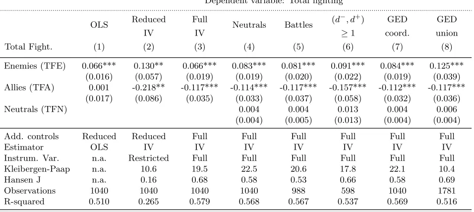
Table1displays the estimates of−βand +γfrom second-stage regressions. Column 1 is an OLS specification. An increase in the enemies’ fighting effort (TFE) is associated with a higher fighting effort, consistent with the theory, whereas an increase in the allies’ fighting effort (TFA) has no significant effect. Since the OLS estimates are subject to an endogeneity bias, in the remaining columns we run a set of IV regressions. Column 2 replicates the specification of column 1 in a 2SLS setup using the lagged fighting efforts of each group’s set of enemies and allies as excluded instruments. In accordance with the predictions of the theory, the estimated coefficients of TFE and TFA are positive (0.13) and negative (-0.22), respectively, and statistically significant at the 5% level.
The associated first-stage regressions are reported in the corresponding columns of Table 2, where, for presentational purposes, only the coefficients of the excluded instruments are displayed. It is reassuring that the lagged rainfall in the enemies’ homelands has a negative effect on the enemies’ (while not on the allies’) fighting effort, whereas the lagged rainfall in the allies’ homelands has a negative effect on the allies’ (while not on the enemies’) fighting effort. This pattern, which conforms with the theoretical predictions, is confirmed in all specifications of Table2. The KP-stat of 10.6 raises a (mild) concern about weak instruments, an issue to which we return below.
In the parsimonious specification of column 2, the coefficients of interest may be affected by some time-varying shocks that affect asymmetrically the armed groups’ incentives to fight. For instance,
(2012). However, neither routine handles spatial correlation in panel IV regressions. 15We owe a special thanks to Rafael Lalive for his generous help in this task.
Table 1: Baseline regressions (second stage).
Dependent variable: Total fighting
OLS Reduced Full Neutrals Battles (d
−, d+) GED GED
IV IV ≥1 coord. union
Total Fight. (1) (2) (3) (4) (5) (6) (7) (8)
Enemies (TFE) 0.066*** 0.130** 0.066*** 0.083*** 0.081*** 0.091*** 0.084*** 0.125*** (0.016) (0.057) (0.019) (0.019) (0.020) (0.022) (0.019) (0.039) Allies (TFA) 0.001 -0.218** -0.117*** -0.114*** -0.117*** -0.157*** -0.112*** -0.117***
(0.017) (0.086) (0.035) (0.033) (0.037) (0.058) (0.032) (0.036)
Neutrals (TFN) 0.004 0.004 0.013 0.004 0.006
(0.004) (0.005) (0.013) (0.004) (0.004)
Add. controls Reduced Reduced Full Full Full Full Full Full
Estimator OLS IV IV IV IV IV IV IV
Instrum. Var. n.a. Restricted Full Full Full Full Full Full
Kleibergen-Paap n.a. 10.6 19.5 22.5 20.6 17.8 22.1 10.4
Hansen J n.a. 0.16 0.68 0.58 0.53 0.66 0.58 0.69
Observations 1040 1040 1040 1040 988 598 1040 1781
R-squared 0.510 0.265 0.579 0.568 0.567 0.537 0.569 0.516
Note: The unit of observation is an armed group in a given year. The panel contains 80 armed groups between 1998 and 2010. All regressions include group fixed effects and control for rainfall in the group’s homeland. Columns 1–3 include time fixed effects. Robust standard errors corrected for spatial HAC in parentheses. Significance levels are indicated by * p<0.1, ** p<0.05, *** p<0.01.
Table 2: Baseline regressions (first stage).
IV regress. of col. (2) IV regress. of col. (3) IV regress. of col. (4)
Dep. Variable: TFE TFA TFE TFA TFE TFA
(1) (2) (3) (4) (5) (6)
Rain (t−1) Enem. -1.595*** -0.019 -1.354*** 0.277* -1.327*** 0.291**
(0.297) (0.141) (0.332) (0.156) (0.322) (0.139)
Sq. Rain (t−1) Enem. 0.000*** 0.000 0.000*** -0.000 0.000*** -0.000 (0.000) (0.000) (0.000) (0.000) (0.000) (0.000)
Rain(t−1)All. 0.126 -0.929*** 0.028 -0.588*** 0.089 -0.571**
(0.283) (0.155) (0.222) (0.192) (0.219) (0.225)
Sq. Rain (t−1) All. -0.000 0.000*** -0.000 0.000*** -0.000 0.000*** (0.000) (0.000) (0.000) (0.000) (0.000) (0.000)
Current Rain Enem. -1.125*** 0.131 -0.936*** 0.073
(0.243) (0.102) (0.257) (0.108)
Sq. Curr. Rain Enem. 0.000*** -0.000*** 0.000* -0.000**
(0.000) (0.000) (0.000) (0.000)
Current Rain All. -0.461** -0.366*** -0.414** -0.448***
(0.204) (0.123) (0.210) (0.164)
Sq. Curr. Rain All. 0.000 0.000*** 0.000 0.000***
(0.000) (0.000) (0.000) (0.000)
Kleibergen-Paap F-stat 10.6 10.6 19.5 19.5 22.5 22.5
Hansen J (p-value) 0.16 0.16 0.68 0.68 0.58 0.58
Observations 1040 1040 1040 1040 1040 1040
global economic or political shocks may change the pressure from international organizations, which in turn affects mainly the war activity of foreign armies, government organizations, or more generally of large combatant groups. To filter out such time-varying heterogeneity, in columns 3–8 we control for three time-invariant characteristics (Government Organization, Foreign, and Large) interacted with a full set of year dummies.17 The description of these three variables can be found in Section 3.2above. Together with adding control variables, we expand the set of excluded instruments (i.e., the rainfall measures), in order to improve the predictive power of the first-stage regression.18 The
expanded set of instruments now comprises current-year and lagged-year rainfall (with a linear and a quadratic term) of allies and enemies, as well as current and lagged rainfall of degree-two neighbors (i.e., enemies’ enemies and allies’ enemies), both with a linear and a quadratic term.19
The estimated coefficients in column 3 continue to feature the alternate sign pattern predicted by the theory. Their magnitude is smaller than in column 2, but the coefficients are estimated more precisely, being statistically significant at the 1% level. In column 4, we add to the vector of regressors TFN (Total Fighting of Neutrals), which is defined in analogy with TFA and TFE. Hence, we now also add to the set of instruments the current and lagged rainfall in the territories of neutral groups (both as a linear and quadratic term). Since the theory predicts that the exogenous variation in TFN should have no effect on the dependent variable, this is a useful test of the theoretical predictions. The prediction is borne out in the data: the point estimate of TFN is very close to zero and statistically insignificant. The first-stage regressions yield large KP-stats (19.5 in column 3 and 22.5 in column 4), suggesting no weak instrument problem. Column 4 is our preferred specification and will be the basis of our robustness checks in the following sections below.
Our measure of fighting intensity is coarse insofar as it does not weigh events by the amount of military force involved. Ideally, we would like to have information about the number of casualties or other measures of physical destruction. However, this information is available only for very few events. This raises the concern that the results may be driven by small events (e.g., local riots or minor skirmishes). As discussed in Section 3.2, ACLED distinguishes between different categories of events. In column 5, we measure fighting effort in a more restrictive fashion, by only counting events that are classified in ACLED as battles. This addresses two issues: first, battles are less likely to get unreported by media; second, it would be reassuring to see that the estimates ofβ and
γ are robust to excluding small events that represent a share of 42% of total events. The estimated coefficients are indeed very similar when we use only information on battles, with no evidence of weak instruments (KP=20.6).20
A related concern is that many of the 80 groups are involved only in a small number of events. Although heterogeneity in group size is controlled for by fixed effects, one might be concerned that the estimation of the externalities hinges on the occasional operation of small groups. In lack of a direct measure of group size, in column 6 we restrict the analysis to the 46 groups that have at least one friend and one enemy, proxying for being relatively important actors. This restriction reduces
17In Section 4.2.3 below, we find that some results are sensitive to the threshold used to construct the dummy variable Large. For this reason, in TableB.2 we replicate Table 1when Large is replaced byLarge 6 (see Section
3.2). The results are robust.
18We also run the specification of column 2 with the expanded set of instruments. The estimated coefficients of interest are 0.15 for TFE (s.e. 0.05) and -0.15 for TFA (s.e. 0.06). The KP-test yields the value 19.7.
19When we use the current and past average rainfall in enemies’ and allies’ homelands as instruments, we also control for the current and past average rainfall in the group’s homeland in the second-stage regression. This is important, since the rainfall in enemies’ and allies’ homelands is correlated with the rainfall in the group’s homeland. Omitting the latter would lead to a violation of the exclusion restriction. The results are robust to including further instruments, for instance, the allies’ allies and the enemies’ allies.
the network size, causing a 40% drop in the number of observations. Reassuringly, the estimated externalities are larger than in column 4 (β= 0.16 and γ = 0.09). The KP-stat is 17.8.
The accuracy of the geolocalization in ACLED has been questioned, as discussed in Section
3.2 above. For this reason, we integrate ACLED with information from the GED, which has been argued to be more accurate in this respect. We cannot simply replace ACLED with GED data because (i) the number of observations would drop by two thirds, aggravating underreporting concerns; (ii) for each event, GED lists at most one group on each side of the clash. However, in 1090 cases it is possible to match events in GED and ACLED beyond reasonable doubt. In these cases, we use the geolocalization in GED to identify the groups’ homelands. For the events that cannot be matched, we continue to use the geolocalization in ACLED. The results, provided in column 7, are indistinguishable from those in column 4 (with KP=22.1).
In addition, we use the union set of the events in GED and ACLED, i.e., we construct a larger dataset that merges the matched events with all unmatched events in either dataset. By this procedure, the number of fighting events increases from 4676 to 5078.21 There is also a larger
number of armed groups, 137 instead of 80. This procedure involves some heroic assumptions, and is subject to the risk that our algorithm fails to match some events that are in fact reported by both datasets, thereby causing an artificial duplication of events. With thiscaveat in mind, we find the estimates of TFE, TFA, and TFN to be, respectively, positive, negative, and insignificant, in accordance with the theory. The order of magnitude of the coefficients is comparable with those in column 4, and the point estimates are in fact larger in absolute value. However, the KP-stat is now lower (10.4). The details of the constructions of the merged dataset are in AppendixC.
The externalities are quantitatively large. Consider the estimates in column 4. The average number of yearly events in which a group is involved is 6, and its standard deviation is 25. Hence, a one standard deviation increase in TFE (i.e., 110 events) translates into a 0.37 increase in total fighting (i.e., 9 events). A one standard deviation increase in TFA (i.e., 86 events) translates into a 0.39 decrease in total fighting (i.e., 10 events). An estimate of the global effect of the network externalities is provided in Section 5.3below.
We have also checked that, conditional on the estimates ofβ and γ,condition (3) holds true for
all groups in conflict in all IV specifications of Table2. Finally, the null hypothesis of the Hansen J test is not rejected in any specification, indicating that the overidentification restrictions are valid.
4.2 Robustness Analysis
We run a large battery of robustness checks. here, we summarize the most important ones.
4.2.1 Variation over Time in the Network Structure
In our dataset, many groups are not active in all periods. We also observe new groups entering the conflict at a later stage, and a few groups which stop fighting. While in the analysis of Section4.1
we interpret zero fighting events as a low fighting effort, the absence of armed engagements could alternatively indicate that a group does not take part in the conflict in a particular subperiod. For this reason, in the first robustness check we address this concern by recognizing that the number of groups that are in the network can change over time.
Table 3: Time-varying network.
Dependent variable: Total fighting
(1) (2) (3) (4) (5) (6) (7)
Total Fight. Enemies (TFE) 0.085*** 0.074*** 0.088*** 0.138*** 0.075 0.068** 0.211*** (0.022) (0.023) (0.024) (0.031) (0.048) (0.030) (0.047) Total Fight. Allies (TFA) -0.115*** -0.097*** -0.106*** -0.212*** -0.143** -0.128*** -0.251***
(0.031) (0.025) (0.030) (0.065) (0.065) (0.041) (0.070) Total Fight. Neutrals (TFN) 0.006 0.003 0.002 0.048** 0.022 0.006 -0.022**
(0.005) (0.004) (0.005) (0.023) (0.021) (0.010) (0.009)
Kleibergen-Paap F-stat 27.1 8.7 11.7 9.2 5.5 15.3 n.a.
Hansen J (p-value) 0.61 0.48 0.60 0.71 0.74 0.51 n.a.
Observations 1040 1040 1040 469 322 637 1040
R-squared 0.603 0.634 0.594 0.501 0.627 0.594 0.179
Note: An observation is a given armed group in a given year. The panel contains 80 armed groups between 1998 and 2010. All regressions include group fixed effects and the full set of controls and instruments (like in baseline column 4 of Table 2). Columns 1-3 define windows of activity and include a group-specific dummy for periods when a group is inactive. In column 1, inactivity is defined by expert coding combined with ACLED information. In column 2, inactivity is defined based on ACLED information only. In column 3, inactivity is based on ACLED information + or - 3 years. Columns 4-6 implement an ILLE estimator on the unbalanced sample of active groups only using the same windows of activity as in columns 1-3. Column 7 performs an instrumented Tobit based on a control function approach. Cluster robust standard errors are corrected for spatial HAC in columns 1–6 and are bootstrapped in column 7. Significance levels are indicated by * p<0.1, ** p<0.05, *** p<0.01.
We use a variety of expert sources to check when each group started its activity, and when, if at all, it ceased to be militarily active. We could gather information for 38 groups (many of them being active in the entire period). However, no official date of establishment or disbandment is available for informal organizations such as ethnic militias. For these groups, we construct a window [S−ω, T+ω],whereS andT are, respectively, the first and last year in which we see the group being active (i.e., xit>0). We add a window of ω ≥0 since the groups might have existed prior to their first or after their last recorded engagement. The details of the construction of the dataset are provided in AppendixC.
We estimate the model by the following three strategies:
1. We add to the baseline specification a set of group-specific dummies switching on in all periods in which the group is suspected to be inactive.
2. We adjust, in addition, the estimation procedure to make it fully consistent with the structural model. To see why, consider equations (4)–(6). When the number of groups in the network changes over time, one must replaceϕ∗i (G) by a time-varying analogue given by
ϕ∗i,t(G;β, γ) = 1− Pn,t 1
i=1Γ β,γ i,t (G)
!
1
Pn i=1Γ
β,γ i,t (G)
!
Γβ,γi,t (G),
where Γβ,γi,t (G) = 1/1 +βdi,t+ −γd−i,t. When ϕ∗i,t is time-varying, it is no longer absorbed by the group fixed effects. However, the model can still be estimated. In particular, one can then estimate the following regression equation:
FIGHTit=FEi+ϕi,t∗ (G;β, γ)−β×TFAit+γ×TFEit−z′itα−ǫit. (16)
alliandt. Thus, we implement the Iterated Linear Least-square Estimator (ILLE) developed by Blundell and Robin (1999).22
3. We estimate the model using instrumented Tobit based on a control function approach.
Table 3 displays the results. All columns report analogues of column 4 in Table 1. Columns 1–3 correspond to the first approach. In column 1, the time window is set to ω = 0; in column 3, we set ω = 3; in column 2, we code as a period of possible inactivity any consecutive spell of zeros at the beginning or at the end of the sample, using only the information from ACLED. The estimates of β and γ are similar to those in column 4 in Table 1. The KP-stats are 25.3, 8.7, and 11.7, respectively. Columns 4–6 correspond to the second approach. In spite of a drastic sample size reduction, the coefficients continue to have the same order of magnitude as in the baseline table. In column 4, the coefficients are larger in absolute value, and the coefficient of TFN turns significant, while remaining much smaller than those of TFE and TFA. In column 5, the coefficient of TFE turns insignificant. In column 6, the results are very similar to column 4 in Table 1. The KP-stats are 6.5, 5.5, and 15.3, respectively. The weak instruments in columns 4 and 5 are not surprising, since the number of observations is, respectively, one third and one half of that in the full sample. Also, this specification is very demanding, since in many cases no reported involvement in ACLED events may indicate a low level of fighting activity rather than an outright withdrawal from the conflict. Column 7 is based on Tobit with a control function approach for the two-stage instrumentation. The estimated coefficients have the usual alternate sign pattern, but are now much larger in absolute value. Overall, we find these results reassuring.
4.2.2 Alternative Specifications
In this section, we consider three sets of robustness checks. All regression tables can be found in AppendixB.
Second-Degree IV, Salient Events, and Alternative Network Construction: A mis-cellany of important robustness checks is summarized in Table B.3. In column 1, we use only the rainfall in the homeland of degree-two neighbors (e.g., the rain of enemies’ enemies and of allies’ enemies) as excluded instruments, following Bramoull´e et al. (2009).23,24 In column 2, we use the
information for the subperiod 1998-2002 to estimate the network links, and the panel for 2003-10 to estimate the spillover coefficients. In columns 3-4, we restrict attention to salient episodes for which measurement error is likely to be less important. In column 3, we drop all events with zero fatalities (while keeping events for which the number is unknown). In column 4, we restrict
22We start by guessing (β
0, γ0) andϕ∗i,t(G;β0, γ0).Then, we obtain a first set of estimates (ˆβ1,ˆγ1) conditional on the guess, update ϕ∗
i,t(ˆβ1,γˆ1),and re-estimate the model iteratively until we converge to a fixed point. Computa-tionally, we stop the iteration as soon ask(ˆβn,γˆn)−(ˆβn−1,ˆγn−1)k<0.0001 (i.e., two orders of magnitude smaller than the estimated standard errors). While Blundell and Robin (1999) address the issue of endogenous regressors with a control function approach (i.e., first stage estimated residuals included as regressors in the second stage), we iterate on our 2SLS estimator that accommodates spatially clustered robust standard errors. We checked that the control function-ILLE and 2SLS-ILLE yield identical point estimates.
23In particular, we continue to treat as excluded instruments the rainfall in the enemies’ enemies’ homelands, the rainfall in the allies’ enemies’ homelands, and the rainfall in the neutrals’ homelands. However, the rainfall in the enemies’ homelands and the rainfall in the allies’ homelands are treated as control variables. For all rainfall measures, we take the linear and square term and the current rain, first lag, and second lag.
attention to battles, riots, and violent events. In column 5, we exclude all events involving group
i when computing the total fighting efforts of allies and enemies of group i. For example, if the LRA’s enemies are involved in 10 clashes in the year 2000, and 3 of them involve the LRA, then the measure of TFE used in the regression would take the value of 7. In column 6, we control for the lagged total fighting effort of both enemies and allies. In columns 7-8, we test the robustness of the results to different definitions of enmities and alliances: in column 7, we code two groups as enemies if they have been observed clashing on at least one occasion, and if they have never been observed co-fighting on the same side; in column 8, we only code two groups as allied if they have been observed co-fighting on at least two occasions during the sample period and if they have had less than two clashes, while analogously we code them as enemies if they have fought on at least two occasions against each other, while having had less than two co-fighting incidents. Further, in column 9, we instrument the network links with dyadic characteristics (co-ethnicity, spatial prox-imity of group centroids, etc.). The observed links are replaced by probabilities of link formation as predicted by a random utility model discussed in Section 6.2 below. Finally, in column 10 we include in the second stage regression the cubic terms of past and current rain.
In terms of results, the coefficient of TFE is always positive, highly significant, and stable. Likewise, the coefficient of TFA is always negative and significant with the exception of column 2. In most cases, the KP-stat is above 20. The coefficient of TFN is always very close to zero and insignificant.
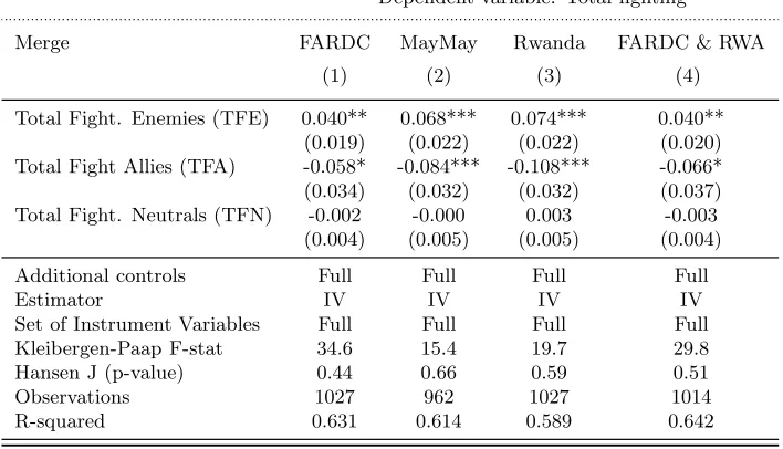
Group Definition (FARDC, Rwanda, & Others): In our benchmark analysis, we have followed the rule of treating groups as separate entities whenever they are classified as such by ACLED. This agnostic way of proceeding has the advantage of not requiring any discretional coding decision. We check the robustness of our results in this dimension.25 In TableB.4, we show
that the results are robust to (i) treating the FARDC-LK and FARDC-JK as one single actor; (ii) merging all local Mayi-Mayi militia branches into one single actor; (iii) merging Rwanda-I and Rwanda-II into a single group; (iv) treating both the FARDC and Rwanda as two single actors.
Ambiguous Network Links: TableB.5deals with ambiguous network links, i.e., links where the narrative might suggest different coding than the one we used. First, we consider the fragile relationship between Uganda and Rwanda (see Section 3.1 for historical background). In our baseline regression, our coding rule classifies Rwanda-I and Uganda as allies (until 1999), whereas Rwanda-II and Uganda are coded as enemies (after 1999). In columns 1 and 2, we code Rwanda and Uganda as always neutral and always allies, respectively. In column 3, instead, we code them as allies until 1999, and as neutral thereafter. Next, we consider another ambiguous relationship, i.e., the FARDC vs. the FDLR. In the baseline estimates, they are first allies (until 2001), and then neutral. Here, we assume that they are enemies after 2001 (column 4), or neutral throughout the entire period (column 5). Other ambiguous network links are discussed in Appendix B. The results are robust.
4.2.3 Alternative Rainfall Data
A concern with our IV strategy is that the rainfall variable may be subject to measurement error. The GPCC data are based on interpolation on information coming from a limited number of gauges in the DRC and neighboring countries. The ensuing classical measurement error could attenuate the power of the rainfall instruments. A potentially more severe problem might arise if the gauge-based