ISSN: 2146-4138 www.econjournals.com
514
Modelling the Macroeconomic Determinants of Workers’ Remittances:
The Case of Jordan
Ghazi Al-Assaf
Business Economics Department, The University of Jordan, Amman 11942, Jordan. Email: [email protected]
Abdullah M. Al-Malki
Department of Administrative Sciences, King Saud University, Riyadh, KSA.
Email: [email protected]
ABSTRACT: This paper explores the main macroeconomic factors, in both host and home countries that affect workers’ remittances. Several macroeconomic variables are taken into account in a cointegration analysis of the long-run relationship among remittances and their macroeconomic determinants as well as the short-run dynamics. The study employs the ARDL and VECM approaches to find out the main macroeconomic determinants that affect remittances to Jordan. Annual data for the period 1972-2009 are used. The empirical results show that macroeconomic factors of host countries are much more significant than home country macroeconomic factors. This confirms the fact that remittances are most likely to be influenced by external factors rather than internal factors. The bounds test used in the ARDL framework indicates that remittances flow to Jordan is cointegrated with the level of income in Jordan, level of income and exchange rates in the host countries. The findings of the study show that the speed of adjustment in the VECM is significant and relatively slow.
Keywords: Workers’ Remittances; Time Series Analysis; Cointegration; ARDL; VECM; Jordan. JEL Classifications: C22; C32; F24
1 Introduction
Workers’ remittances – the portion of migrant workers’ earning sent back from the country of employment to the country of origin- are considered a magnificent part of international capital flows between countries especially in the case of labour exporting country such as Jordan. Remittances are becoming an important and stable source of external flows in the Middle East over the last two decades. They play an increasingly important role in international economic relations between poorer, labour exporting, countries and labour scarce richer countries, see Russell (1986). Remittances are also becoming a main source for developing and enhancement of economic stability in the economy through providing an extra income to the families that benefited from these transfers.
In addition, the lack of capital inflows in developing countries, particularly Jordan, makes remittances an important factor, in place of foreign capital. However, remittances also provide an increasingly valuable source of extra saving and capital accumulation. Therefore, economics of remittances has become an area of interest over the last two decades. Many of the studies concerning remittances investigate their impact on various economic variables. In some studies, the emphasis is placed on the determinants of the flows of remittances. They investigate the main factors that influence workers’ remittances. However, there is no study in the literature exclusively devoted to the remittances from Jordanian expatriates working abroad. This paper is one of the first that investigates this issue.
515 influenced by different variables in two main countries of the Arabian Gulf. Recorded numbers of the Jordanian expatriates show that more than 75 % work in Saudi Arabia and the United Arab of Emirates (UAE)1. These countries are the biggest host countries of the Jordanian expatriates. Therefore, the models used in this paper take into account certain macroeconomic variables in Saudi Arabia and UAE to investigate whether these variables have a significant impact on the flows of remittances to Jordan (see Al-Assaf, 2012).
The study is organised as follows. Next section presents the general trend in remittance flows to Jordan. Section 3 provides a brief background of previous work regarding the topic under investigation, while section 4 presents the methodology and data used in this paper, the empirical results of the cointegration analysis, which include both the ARDL and VECM frameworks are discussed in section 5. Finally, section 6 concludes.
2 Trend in the Jordanian Workers’ Remittances
The concept of workers’ remittances as defined in the International Monetary Fund (IMF) interpretation refers to the value of monetary transfers sent home from workers residing abroad for more than one year, and it is recorded in different sections of the balance of payments. In this part of the study we present briefly the general trend in workers remittance flows to Jordan
The money that migrants send home, remittances, represent today an important source of external funding for many developing countries, including Jordan. According to the World Bank data on remittances, with about 2800 billion USD in 2009, Jordan ranks at 10th place among all developing countries. Jordan has ranked constantly among the top 20 remittances-recipient countries over the last decade. In addition, the Arab Monetary Fund (AMF) statistics in 2009 indicate that Jordan was the second biggest recipients of remittances among Arab countries after Lebanon. This confirms the fact that remittance flows to Jordan are considered a great area of interest.
The following figure shows the general trend in remittance flows to Jordan over the period 1972-2009. It can be seen that Jordan has reported a spectacular increase in remittance flows over the 1970s and the first half of the 1980s, where remittance flows had increased from 20.7 million USD in 1972 to more than 600 million USD in 1979 and then to about 1237 million USD in 1984 (see figure 1). The main factors for this remarkable increase is that the number of migrants to the Arabian Gulf Countries had grown sharply during that time, where thousands of the Jordanian skilled workers migrated to the Arabian Gulf Countries, especially during the oil boom in the Gulf Countries in 1970s and 1980s. Over the second half of the 1980s, remittances had dropped gradually as a result of the economic crisis that happened during that period. This was a consequence of the sharp drop in oil prices and its impact on the economic development in the labour-imported countries, where these flows dropped about 30% in 1989 comparing with their level in 1988.
Figure 1. Remittance Flows to Jordan Over 1972-2008
516 After that, the flows of remittance to Jordan had experienced rapid growth rates particularly over the years 1992 and 1993; the growth rate reached 88% in 1992, where Jordan had started again exporting high skilled labour after the Gulf War. This increase had continued steadily over the period 1995-2004, where the average growth rate was 7% for that period. In the last two years, the remittance flows have reached high levels at 2514 and 2835 in 2006 and 2007, respectively. The annual average growth rate of recorded remittances was 14% for these years. It is also seen that remittances in Jordan have started to affect many of the macroeconomic variables in Jordan, especially the financial ones, see Al-Tarawneh and Al-Assaf (2013).
3 Literature Review
Most of previous studies about the determinants of remittances have investigated microeconomic factors that determine the flows of remittances. A few studies have extensively focused on macroeconomic determinates of remittances such as Swamy (1981), Lianos (1997), El-sakka and MacNabb (1999), Glytsos (2002), Gupta (2005), and Shahbaz and Aamir (2009). Some of these studies have argued that macroeconomic variables in the home country have significant effects on the remittances such as level of income, inflation, and exchange rate.
In addition, most of the previous papers have found that remittances respond significantly to the behaviour of macroeconomic variables in the host country rather than the home country, see Huang and Silva (2006) and Elbadawi and Rocha (1992). Therefore, the level of income, the exchange rate, and the inflation of host countries are expected to have a significant impact in our case. However, the main challenging aspect of the study of remittances at macro level is related to data collection as the variables that might affect these flows vary from country to country.
4 The Methodology and Data 4.1 The Methodology
The answer to the question whether macroeconomic variables might affect the flow of remittances to Jordan can be obtained from cointegration analysis. The advantage of testing for cointegration is the identification of a stable long run relationship between remittance flows and these variables, which could be implemented using various cointegration methodologies. The main framework of our analysis is based on Autoregressive Distributed Lag (ARDL) and Vector Error Correction Model (VECM) methodologies. The general specification of the model used in our analysis is based on the following equation:
= (1)
Where: is workers’ remittances to Jordan, are macroeconomic determinants of workers’ remittances from four countries, and is the error term.
The analysis then continues using these two cointegration approaches. First, the ARDL model is used to examine the long-run relationship among the series. Second, the VECM is estimated to explore the short- and long-run dynamics between remittances and its determinants.
4.2 Data and Variables
Despite the highly increased interest in investigating workers’ remittances, relatively little work has been done to improve the understanding of the macroeconomic determinants of remittance flows. The main reasons for this are the scarcity and inaccuracy of data. Most previous work has investigated microeconomic determinants of remittances relying on survey data. Alternatively, researchers have used IMF balance of payments data to investigate macroeconomic determinants. In our case we have used data published by the IMF as well as the world development indicators published by the World Bank, and the yearly bulletins of the central banks of Jordan and host countries. The descriptive statistics and matrix correlation of the used variables are reported in table 2 and 3, respectively, in the appendix.
517 For cointegration analysis we use annual data covering the period 1972-2009 for all series. In our estimation we use annual data rather than quarterly data containing more observations over the same period, because it is now well-known that unit root and cointegration tests require a long time span of data rather than merely a large number of observations. There is no gain in switching from low frequency to high frequency data and merely increasing the number of observations, see Campbell and Perron (1991); and Demetriades and Hussein (1996).
5 Empirical Evidence 5.1 Unit root Testing
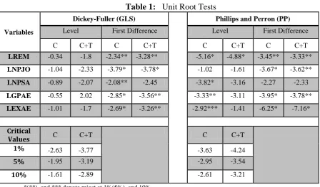
We start the empirical investigation by performing unit root tests to determine whether the series used in the analysis are stationary in levels. We have applied both Dickey-Fuller (GLS)(DF-GLS) and Phillips and Perron (PP) tests for the variables under investigation. Both tests results indicate that all variables are nonstationary at levels and stationary at first differences (results are reported in Table 1 in appendix). Thus, workers’ remittances and other macroeconomic determinants are integrated of the same I(1) order. As these series are integrated, our next step is to investigate whether a long-run relationship exists among the variables. This can be found through using different cointegration techniques such as ARDL and VECM frameworks.
5.2 Autoregressive Distributed Lag (ARDL):
Empirical studies that contain a set of time series may employ spurious regression. The cointegration framework developed by Engle and Granger (1987) overcomes this problem. Nevertheless, their approach becomes invalid if there are more than one cointegration vector in the system. Bounds test approach developed by Pesaran et al. (2001) provides a method for cointegration testing when some series are stationary. The cointegration relationship can be tested among the series, regardless of whether they are I(0) or I(1). Both approaches assume one cointegration relationship. Here we use the ARDL approach, suggested by Pesaran and Shin (1995), to estimate the long run relationship among a set of variables including workers’ remittances and potential macroeconomic determinants. We have also employed the Engle-Granger two-step procedure and the results (not fully reported here) indicate that there is a significant long-run relationship between workers’ remittances to Jordan (LREM) and macroeconomic determinants, namely LNPJO, LNPSA, LEXAE, and LGPAE (defined below). 2 We consider the ARDL model to test for a long run relationship among variables. The orders of the lags in the ARDL model are selected by using either the Akaike Information Criterion (AIC) or the Schwarz Bayesian Criterion (SBC), before the selected model is estimated by ordinary least squares. For annual data, Pesaran and Shin (1999) recommended choosing a maximum of 2 lags. From this, the lag length that minimizes SBC is selected, which is one in this context, the optimal lag length selection criteria are presented in Table 4 in the appendix. According to this approach, we first consider the following ARDL (1, 1, 1, 1, and 1) equation:
Where: LREM: log of remittance flows to Jordan, LNPJO: log of GNI per capita for Jordan, LNPSA: log of GNI per capita in Saudi Arabia, LGPAE: log of GDP per capita in United Arab of Emirates,
LEXAE: log of exchange rate in UAE, and : the error term, where these variables include the main significant variables that might affect the flows of remittances to Jordan. Table (1) contains the empirical results of this regression.
2 Where the stationarity test of the residual obtained from the equilibrium regression indicates that we reject the
518
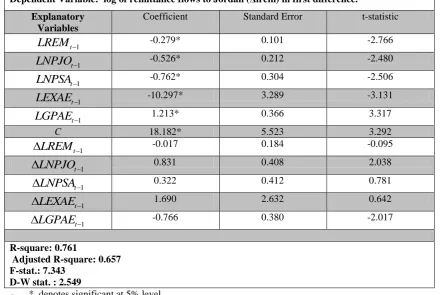
Table 1. ARDL Estimation of the Macroeconomic Determinants of Remittances
Dependent Variable: log of remittance flows to Jordan (Δlrem) in first difference.
Explanatory Variables
Coefficient Standard Error t-statistic
1
t
LREM
-0.279* 0.101 -2.7661
t
LNPJO
-0.526* 0.212 -2.4801
t
LNPSA
-0.762* 0.304 -2.5061
t
LEXAE
-10.297* 3.289 -3.1311
t
LGPAE 1.213* 0.366 3.317
C 18.182* 5.523 3.292
1
t
LREM
-0.017 0.184 -0.0951
t
LNPJO
0.831 0.408 2.0381
t
LNPSA
0.322 0.412 0.7811
t
LEXAE
1.690 2.632 0.6421
t
LGPAE
-0.766 0.380 -2.017
R-square: 0.761
Adjusted R-square: 0.657 F-stat.: 7.343
D-W stat. : 2.549
- * denotes significant at 5% level.
From Table (1), some of the variables are not significant especially the first difference of income level in Saudi Arabia, exchange rate in the UAE, and remittance flows lagged. We re-specify the ARDL model by dropping the insignificant variables. We estimate the following reduced ARDL model, (parsimonious ARDL (1, 1, 1, 1, and 1)):
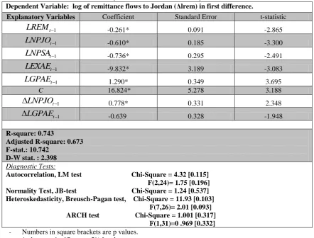
The empirical results are presented in Table (2). These results indicate that income levels in Jordan and Saudi Arabia have significant negative effects on remittances in the long-run. However, the results show a positive impact of the level income in UAE on these remittances. Also, the exchange rate of the Emirates Dirham against the US dollar affects the flows of remittances to Jordan negatively.
Various diagnostic tests have to be applied to confirm the validity of the model. We implement various residual tests, starting with the LM test for serial correlation, which is a general test for serial correlation. The LM test statistic for the null hypothesis of no serial correlation clearly indicates that there is no serial correlation in the residuals. To test for heteroskedasticity, we employ the Breusch-Pagan test. All diagnostic tests are shown at the bottom panel of Table (2).
The results indicate that the growth of remittances over the time can be explained by the level of income or the economic situation expressed by the GNI per capita in Jordan, especially in the short-run. This is consistent with the finding of Gupta (2005); growth in the economy of the home country simulates remittances to Jordan. In particular, it encourages the Jordanian expatriates to transfer their money through official channels, rather than unofficial ones when the economy is improving. This explains the positive sign of the ΔLNPJO coefficient.
519
Table 2. ARDL Estimation of the Macroeconomic Determinants of Remittances (The Parsimonious Model)
Dependent Variable: log of remittance flows to Jordan (Δlrem) in first difference.
Explanatory Variables Coefficient Standard Error t-statistic
1
t
LREM
-0.261* 0.091 -2.8651
t
LNPJO
-0.610* 0.185 -3.3001
t
LNPSA -0.736* 0.295 -2.491
1
t
LEXAE
-9.832* 3.189 -3.0831
t
LGPAE
1.290* 0.349 3.695C 16.824* 5.278 3.188
1
t
LNPJO
0.778* 0.331 2.3481
t
LGPAE
-0.639 0.328 -1.948
R-square: 0.743
Adjusted R-square: 0.673 F-stat.: 10.742
D-W stat. : 2.398
Diagnostic Tests:
Autocorrelation, LM test Chi-Square = 4.32 [0.115] F(2,24)= 1.75 [0.196] Normality Test, JB-test Chi-Square = 1.24 [0.537] Heteroskedasticity, Breusch-Pagan test, Chi-Square = 11.93 [0.103] F(7,26)= 2.01 [0.093] ARCH test Chi-Square = 1.001 [0.317] F(1,31)=0 .969 [0.332]
- Numbers in square brackets are p values. - * denotes significant at 5% level.
The bounds error correction test is calculated from an estimated unrestricted error-correction model (UECM), the version of the ARDL model, by Ordinary Least Square (OLS) see Pesaran et al. (2001). This test is the Wald test (F-statistic version of the bounds testing approach) for the lagged level variables in the right-hand side of the UECM, Greene (2003). We test the null hypothesis of no cointegration relationship among the variables by conducting a joint significance test on lagged level variables. The null states the coefficients of all lagged level variables in the model are equal to zero. The distribution of this F-statistic is non-standard under the null hypothesis. The basic hypothesis is as follows:
Null : against Alternative : At least some are non zero.
We then compare the calculated F statistic with critical bounds values (lower and upper values). A conclusive inference can be made without considering the order of integration of the explanatory variables. If the F-statistic is higher than the upper critical bound, the null hypothesis of no cointegration between series is rejected and hence there is a cointegration relationship between the variables. If the test statistic is below the lower critical bound, we cannot reject the null hypothesis and the conclusion of no cointegration relationship remains. Finally, if the calculated F statistic is between the upper and lower bounds the test cannot give conclusive inference; see Pesaran et al. (2001).
Table 3. Bounds Test for Cointegration
Calculated F-Statistics 8.689*
Bound Testing Critical Values3 at 5% 2.62 (Lower)
3.79 (Upper) * Denotes rejection the null at 5% level of significance.
3
520 It can be seen from Table 3 that the calculated F-statistic is 8.689 which is exceed the upper critical bound (3.79) at 5% significance level. It is also exceeds the upper critical bound at 1% significance level (4.68). This implies that the null hypothesis of no cointegration is rejected.
Given a cointegration relationship between remittance flows to Jordan and the considered macroeconomic variables in both home and host countries, a VECM can also be used to determine long and short-term relationships. We explore this in the following section.
5.3 Vector Error Correction Model (VECM):
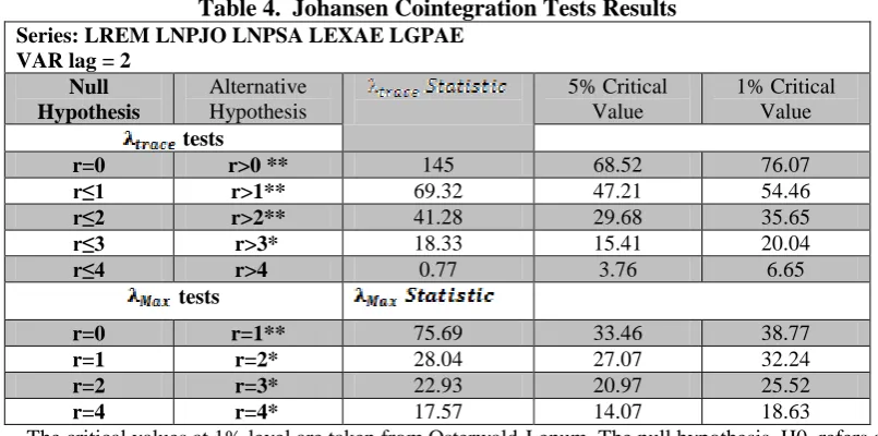
We continue our analysis to test whether the series under investigation are cointegrated over the time. The Johansen maximum likelihood test (1988) is used to test for the presence of cointegration among variables. The test results are shown in Table (4).
Table 4. Johansen Cointegration Tests Results
Series: LREM LNPJO LNPSA LEXAE LGPAE VAR lag = 2
Null Hypothesis
Alternative Hypothesis
5% Critical Value
1% Critical Value
tests
r=0 r>0 ** 145 68.52 76.07
r≤1 r>1** 69.32 47.21 54.46
r≤2 r>2** 41.28 29.68 35.65
r≤3 r>3* 18.33 15.41 20.04
r≤4 r>4 0.77 3.76 6.65
tests
r=0 r=1** 75.69 33.46 38.77
r=1 r=2* 28.04 27.07 32.24
r=2 r=3* 22.93 20.97 25.52
r=4 r=4* 17.57 14.07 18.63
- The critical values at 1% level are taken from Osterwald-Lenum. The null hypothesis, H0, refers at most r cointegrating vectors when r is the order of cointegraion.
- * and ** represent significant at 5% and 1% respectively.
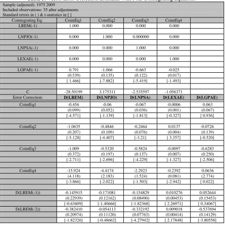
Both trace and maximum-eigenvalue tests suggest at least four cointegration vectors4. This is evidence that there may be long-run relationships among the series.
Having found at least one cointegration relationship between remittance flows and related macroeconomic variables a VECM model with one cointegrating vector is used5. It is useful to consider specific parameterisations that support the analysis of the cointegration structure. The VAR can be constructed in terms of the levels of data or in terms of their differences with the addition of an error correction term (ECT) to capture the long run dynamics. The resulting model is known as a VECM or as it is sometimes called a vector equilibrium correction model, see Banerjee et al. (1993) and Lutkepohl and Kratzig (2004).
As a starting point, we can set a VECM for the macroeconomic determinants of workers’ remittances. Since the data are in annual basis, we choose two for the maximum order of lags in the model; therefore the model will be constructed as follows:
j= 1, 2,..., k.
4 For more details about these tests see: Harris (1995) and Crompbell (1995, pp. 76-80 and pp. 19) respectively. 5 The present empirical analysis is based on imposing one cointegrating vector. Further analysis imposing two or
521 Where represents the flows of remittances to Jordan, and represents macroeconomic determinants that might affect remittances. and are the differences in the variables that capture short-run dynamics, and are serially uncorrelated error terms, and is the error correction term, derived from the long run cointegration relationship and measures the magnitude of the past disequilibrium, where the coefficients of this error correction term ( ) reflect the deviation of the dependent variables from the long run equilibrium.
Below we only discuss equation (4) of the VECM. It contains four variables including income level for home countries expressed by the log of gross national income per capita (lnpjo), gross national income per capita (lnpsa) and gross domestic product per capita (lgpae) in both Saudi Arabia and UAE respectively which serve as a proxy for the income levels for migrants, and exchange rate in UAE6. Our specific error correction model is based on the following equation:
Where the model contains the main macroeconomic variables that have been found to have a quite significant impact on the flows of remittances to the Jordanian economy. Equation (6) represents a VECM of the determinants of remittances. The results are presented in table (5) and (6) for both long-run and short-long-run coefficients respectively, with the required diagnostic test below.
Table 5. VECM Estimation of Macroeconomic determinants of Remittances ( Long-run Coefficients)
Dependent Variable: log of remittance flows to Jordan (Δlrem) in first difference. Explanatory
Variables
Coefficient Standard Error t-statistic
1
t
LNPJO
4.603* 0.514 8.9581
t
LNPSA
2.983* 0.819 3.6411
t
LEXAE
12.493* 5.610 2.2271
t
LGPAE -6.420* 0.837 -7.669 C -34.646* 0.050 3.486 - * denotes significant at 5% level.
The optimal lag length is selected based on various statistics, including the Akaike Information Criterion (AIC), the Hannan-Quin Criterion (HQ) and Schwarz Criterion (SQ). From these criteria, we conclude that the optimal lag length should be two.
From Table (5), results show that, in the long-run, remittances are positively related to the level of income in Jordan and Saudi Arabia, and the exchange rate of the UAE, while the income level of the Jordanian expatriates, working in the UAE, has a significant negative effect in the long run. The most important point is that we find a significant relationship between remittances and exchange rate in the host country, whereby the exchange rate of the UAE is found to affect remittances positively. Other studies find the opposite, that is the exchange rate of the home country is important, see Lianos (1997), El-sakka and Macnabb (1999), and Shahbaz and Aamir (2009).
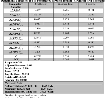
In addition, estimation of short run dynamics based on VECM are presented in table (6), giving the short-run fluctuations of remittance flows to Jordan. It is noticed that macroeconomic variables in both host and home country are found to have insignificant effects on remittance flows in the short-run.
6
522
Table 6. VECM Estimation of Macroeconomic determinants of Remittances (Short-run Coefficients)
Dependent Variable: log of remittance flows to Jordan (Δlrem) in first difference.
Explanatory Variables
Coefficient Standard Error t-statistic
1
t
LREM
-0.049 0.255 -0.1912
t
LREM
-0.574* 0.245 -2.346
1
t
LNPJO
0.602 0.475 1.269
2
t
LNPJO
0.943 0.512 1.8421
t
LNPSA
-0.376 0.556 -0.6772
t
LNPSA
0.293 0.468 0.6261
t
LEXAE
12.919 7.207 1.793
2
t
LEXAE
-1.812 3.383 -0.536
1
t
LGPAE
-0.222 0.318 -0.6982
t
LGPAE
-0.296 0.362 -0.820C 0.176* 0.050 3.486 ECT -0.162* 0.044 -3.681
R-square: 0.749
Adjusted R-square: 0.618 Standard error: 0.160 F-stat.: 5.713
Log likelihood: 21.053 Akiake AIC: -0.549 Schwarz SC: -0.0045
Diagnostic Tests:
Autocorrelation, LM test (12) 25.79 [0.42] Normality Test, JB-test 19.84 [0.031] Heteroskedisticity, White test, 350.4 [0.211]
- Numbers in square brackets are p values. - * denotes significant at 5% level.
The error correction term (ECT) has coefficient -0.162, with a negative significant direction. This coefficient is also called the adjustment coefficient or speed of convergence and it implies that when remittances deviate from long run equilibrium, error correction term has an opposite adjustment effect and the deviation degree is reduced. Thus, the change will move towards stationarity. This also implies that the convergence term is quite slow in our results.
We apply a number of diagnostic tests to the residual of the VECM; they are shown at the bottom of Table (6). The LM test implies that there is no serial correlation problem in the error. Moreover, the normality test suggests evidence of non-normality. Finally, the White test suggests that there is no heteroskedasticity problem in the model. As a result, we can conclude that the vector error correction model, used in our analysis, passes the required diagnostic tests.
6 Conclusion
In this paper, we investigate empirically the long run relationship between remittance flows to Jordan and macroeconomic determinants that might affect these flows. In particular, we have confirmed the fact that remittance flows are caused by income levels of migrants in the host country rather than income level in home country.
The empirical results indicate that there is a stable long run equilibrium relationship among the flows of remittances to Jordan and the macroeconomic variables in host countries, particularly Saudi Arabia and UAE.
523 some previous studies, we find that exchange rates as well as level of income are important factors in affecting remittance flows to Jordan. However, we could not find any significant effects of interest rate and inflation in both home and host countries on the Jordanian remittances. This finding is considered as a very important issue that would open the gate for the Jordanian decision makers to implement more coordination with the host countries.
References
Al-Assaf, G. (2012). Workers’ Remittances in Jordan. Germany, LAMBERT Academic Publishing. Al-Tarawneh, A., Al-Assaf, G. (2013). Do Workers’ Remittances Promote Banking Sector
Development in Jordan? International Research Journal of Finance and Economics, 117, 37-54. Banerjee, A., Dolado, J., Galbraith, J.W., Hendry, D.F. (1993) Co-Integration, Error-Correction, and
the Econometric Analysis of NonStationary Data. Oxford: Oxford University Press.
Campbell, J., Perron, P., 1991. Pitfalls and opportunities: what macroeconomists should know about unit roots. In: Blanchard, O., Fischer, S. (Eds.), NBER Macroeconomics Annual. MIT Press, Cambridge, MA.
Demetriades, P.O., Hussein, A.K. (1996) Does Financial Development Cause Economic Growth? Time Series Evidence from 16 Countries. Journal of Development Economics, 51, 387–411. Department of International Cooperation, Ministry of Labour, Amman, Jordan
Elbadawi, I., Rocha, R. (1992). Determinants of Expatriates Workers' Remittances in North Africa and Europe. World bank Working Paper 1038, Washington, D.C.
El-sakka, M.I.T., Mcnabb, R. (1999). "The Macroeconomic Determinants of Emigrant Remittances."
World Development, 27(8), 1493-1502.
Engle, R.F., Granger, C.W.J. (1987), Cointegration and Error Correction: Representation, Estimation, and Testing, Econometrica, 55(2), 251-76.
Engle, R., Yoo, S. (1987), Forecasting and testing in cointegrated systems, Journal of Econometrics, 35, 143–159.
Gupta, P. (2005). "Macroeconomic Determinants of Remittances: Evidence from India." IMF Working Paper, Dec 2005(224).
Glytsos, N.P. (2002). "A Model of Remittances Determination Applied to Middle East and North Africa Countries." Centre of Planning and Economic Research 73(April).
Greene, W. (2003), Econometric Analysis. 5th edition, Prentice Hall, New Jersey.
Harris, R. (1995). Using Cointegration Analysis in Econometric Modelling. London, Prentice Hall. Huang, P., Silva, C. (2006). Macroeconomic determinants of workers' remittances: Host versus home
country's economic conditions, Journal of International Trade & Economic Development, 15(1), 81-99.
Johansen, S. (1988). Statistical analysis of cointegration vectors. Journal of Economic Dynamics and Control, 12(2-3), 231-254.
Lianos, T.P. (1997). "Factors Determining Migrant Remittances: the case of Greece." International Migration Review, 31(1), 72-87.
Lutkepohl, H., Kratzig, M. (2004). Applied Time Series Econometrics. Cambridge, Cambridge University Press.
Pesaran, M.H., Shin, Y. (1995) “An Autoregressive Distributed Lag Modelling Approach to Cointegration Analysis.” DAE Working Paper, No. 9514, Department of Applied Economics, University of Cambridge,
Pesaran, M.H., Shin, Y., Smith, R.J. (2001)“Bounds Testing Approaches to the Analysis of Long-Run Relationship.” Journal of Applied Econometrics, 16, 289–326.
Russell, S. (1986). Remittances from International Migration: A Review in Perspective. World Development, 14(6), 677-696.
Shahbaz, M., Aamir, N. (2009). "Determinants of Workers' Remittances: Implication for Poor People of Pakistan." European Journal of Scientific Research, 25(1), 130-144.
Swamy, G. (1981). International Migration Workers' Remittances: Issues and Prospects. World Bank Working Paper 481.
Thagunna, K., Achary, S. (2013). “Empirical Analysis of Remittance Inflow: The Case of Nepal."
524
A
A
P
P
P
P
E
E
N
N
D
D
I
I
X
X
Table 1: Unit Root Tests
Variables
Dickey-Fuller (GLS) Phillips and Perron (PP)
Level First Difference Level First Difference
C C+T C C+T C C+T C C+T
LREM -0.34 -1.8 -2.34** -3.28** -5.16* -4.88* -3.45** -3.33**
LNPJO -1.04 -2.33 -3.79* -3.78* -1.02 -1.61 -3.67* -3.62**
LNPSA -0.89 -2.07 -2.08** -2.45 -3.82* -3.16 -2.27 -2.33
LGPAE -0.55 2.02 -2.85* -3.56** -3.33** -3.11 -3.95* -3.78**
LEXAE -1.01 -1.7 -2.69* -3.26** -2.92*** -1.41 -6.25* -7.16*
Critical
Values C C+T C C+T
1% -2.63 -3.77 -3.63 -4.24 5% -1.95 -3.19 -2.95 -3.54 10% -1.61 -2.89 -2.61 -3.21
- *(**), and *** denote reject at 1%(5%), and 10%.
- C: represents test with constant, C+T: represents test with constant and trend.
Table 2: Descriptive Statistics
LREM LNPJO LNPSA LEXAE LGPAE
Mean 20.5 7.34 9.03 1.32 9.86
Median 20.78 7.41 9.04 1.30 9.85
Maximum 21.76 7.96 9.77 1.48 10.72
Minimum 16.85 6.11 7.26 1.30 8.47
Std. Dev. 1.09 0.44 0.51 0.04 0.40
Skewness -1.81 -1.23 -1.83 2.46 -0.99
Kurtosis 6.06 3.99 7.33 9.03 6.42
Jarque-Bera 33.64 10.51 48.08 90.68 23.41
Probability 0.00 0.005 0.000 0.000 0.000
Sum 737.96 264.33 325.07 47.46 355.09
Sum Sq. Dev. 41.79 6.77 9.035 0.054 5.65
Observations 38 38 38 38 38
Table 3: Matrix Correlation
LREM LNPJO LNPSA LEXAE LGPAE
LREM 1 0.911 0.831 -0.887 0.709
LNPJO 1 0.843 -0.864 0.699
LNPSA 1 -0.766 0.882
LEXAE 1 -0.579
525
Table 4: Lag Order Selection Criteria for the ARDL
Sample: 1972 2009
Included observations: 35
Lag LogL LR FPE AIC SBC HQ
0 86.91421 NA 5.56e-09 -4.818483 -4.594018 -4.741934
1 283.4618 323.7255 2.35e-13 -15.70952* -13.56273* -14.45022
2 323.3149 53.91891* 1.08e-13* -14.98323 -13.31412 -14.94119*
* indicates lag order selected by the criterion
LR: sequential modified LR test statistic (each test at 5% level)
FPE: Final prediction error AIC: Akaike information criterion
SBC: Schwarz information criterion HQ: Hannan-Quinn information criterion
Table 5: Vector Error Correction Estimates with Four Cointegrating Equations
Sample (adjusted): 1975 2009
Included observations: 35 after adjustments Standard errors in ( ) & t-statistics in [ ]
Cointegrating Eq: CointEq1 CointEq2 CointEq3 CointEq4
LREM(-1) 1.000 0.000 0.000 0.000
LNPJO(-1) 0.000 1.000 0.000000 0.000
LNPSA(-1) 0.000 0.000 1.000 0.000
LEXAE(-1) 0.000 0.000 0.000 1.000
LGPAE(-1) 0.791 -1.066 -0.663 -0.025
(0.539) (0.135) (0.122) (0.017)
[ 1.466] [-7.882] [-5.419] [-1.493]
C -28.50199 3.175311 -2.535597 -1.056371
Error Correction: D(LREM) D(LNPJO) D(LNPSA) D(LEXAE) D(LGPAE)
CointEq1 -0.456 -0.06 -0.067 -0.0006 0.063
(0.099) (0.052) (0.036) (0.001) (0.067)
[-4.571] [-1.139] [-1.813] [-0.327] [ 0.936]
CointEq2 -1.0635 -0.4846 -0.2464 0.0137 -0.0726
(0.207) (0.109) (0.076) (0.004) (0.139)
[-5.128] [-4.407] [-3.21] [ 3.357] [-0.520]
CointEq3 -1.009 -0.5320 -0.5824 -0.0097 -0.6283
(0.372) (0.197) (0.137) (0.007) (0.250)
[-2.711] [-2.696] [-4.229] [-1.327] [-2.506]
CointEq4 -15.924 -4.4174 -2.2923 -0.2392 0.0636
(4.118) (2.183) (1.524) (0.081) (2.774)
[-3.866] [-2.022] [-1.503] [-2.942] [ 0.022]
D(LREM(-1)) -0.145915 -0.171081 -0.154829 0.010276 0.052644
(0.22939) (0.12162) (0.08490) (0.00453) (0.15453)
[-0.63609] [-1.40666] [-1.82368] [ 2.26971] [ 0.34067]
D(LREM(-2)) -0.382410 -0.054113 -0.332192 0.009018 -0.537694
(0.20974) (0.11120) (0.07763) (0.00414) (0.14129)
526
D(LNPJO(-1)) 1.288715 0.610250 0.295871 -0.008495 -0.350346
(0.47800) (0.25343) (0.17691) (0.00943) (0.32200)
[ 2.69608] [ 2.40799] [ 1.67245] [-0.90040] [-1.08803]
D(LNPJO(-2)) 1.503918 0.507834 0.643352 -0.020262 0.895020
(0.45228) (0.23979) (0.16739) (0.00893) (0.30468)
[ 3.32521] [ 2.11782] [ 3.84344] [-2.26988] [ 2.93761]
D(LNPSA(-1)) 0.263527 0.543835 0.302107 -0.024161 0.531028
(0.48819) (0.25883) (0.18068) (0.00964) (0.32887)
[ 0.53980] [ 2.10109] [ 1.67203] [-2.50745] [ 1.61470]
D(LNPSA(-2)) 0.125005 -0.033308 0.203489 0.007368 0.495697
(0.43495) (0.23060) (0.16098) (0.00858) (0.29300)
[ 0.28740] [-0.14444] [ 1.26409] [ 0.85831] [ 1.69178]
D(LEXAE(-1)) 18.57217 3.663173 -1.067160 0.126439 -0.383914
(6.89851) (3.65749) (2.55316) (0.13616) (4.64717)
[ 2.69220] [ 1.00155] [-0.41798] [ 0.92863] [-0.08261]
D(LEXAE(-2)) 2.922943 0.497949 1.333360 -0.204924 -1.464931
(3.85163) (2.04208) (1.42550) (0.07602) (2.59464)
[ 0.75889] [ 0.24384] [ 0.93536] [-2.69567] [-0.56460]
D(LGPAE(-1)) -0.899398 -0.865553 -0.215624 0.009141 -0.424874
(0.42156) (0.22350) (0.15602) (0.00832) (0.28398)
[-2.13351] [-3.87264] [-1.38202] [ 1.09865] [-1.49613]
D(LGPAE(-2)) -0.619446 -0.573469 -0.240047 0.019739 -0.779790
(0.35999) (0.19086) (0.13323) (0.00711) (0.24251)
[-1.72072] [-3.00460] [-1.80168] [ 2.77808] [-3.21551]
C 0.163679 0.076246 0.059166 -0.004908 0.063118
(0.04301) (0.02280) (0.01592) (0.00085) (0.02897)
[ 3.80552] [ 3.34356] [ 3.71678] [-5.78110] [ 2.17840]
R-squared 0.856 0.797 0.933 0.919 0.719
Adj. R-squared 0.744 0.6406 0.881 0.856 0.501
Sum sq. resids 0.310 0.087 0.042 0.000 0.141
S.E. equation 0.131 0.069 0.048 0.002 0.088
F-statistic 7.632 5.074 17.96 14.66 3.297
Log likelihood 30.16 51.10 62.96 159.7 43.2
Akaike AIC -0.919 -2.188 -2.90 -8.769 -1.709
Schwarz SC -0.239 -1.508 -2.226 -8.089 -1.029
Mean dependent 0.109 0.044 0.043 -0.002 0.029
S.D. dependent 0.259 0.116 0.141 0.006 0.125
Determinant resid covariance (dof adj.) 2.60E-15
Determinant resid covariance 1.26E-16
Log likelihood 370.01
Akaike information criterion -16.66