Gaussian
Beam Optics
Optical Specifications
Material Pr
operties
Optical Coatings
Introduction 1.2
Paraxial Formulas 1.3
Imaging Properties of Lens Systems 1.6
Lens Combination Formulas 1.8
Performance Factors 1.11
Lens Shape 1.17
Lens Combinations 1.18
Diffraction Effects 1.20
Lens Selection 1.23
Spot Size 1.26
Aberration Balancing 1.27
Definition of Terms 1.29
Paraxial Lens Formulas 1.32
Principal-Point Locations 1.36
Prisms 1.37
Polarization 1.41
Waveplates 1.46
Etalons 1.49
Ultrafast Theory 1.52
Fundamental Optics
Gaussian Beam Optics
Optical Specifications
Material Pr
operties
Introduction
The process of solving virtually any optical engineering problem can be broken down into two main steps. First, paraxial calculations (first order) are made to determine critical parameters such as magnification, focal length(s), clear aperture (diameter), and object and image position. These paraxial calculations are covered in the next section of this chapter.
Second, actual components are chosen based on these paraxial values, and their actual performance is evaluated with special attention paid to the effects of aberrations. A truly rigorous performance analysis for all but the simplest optical systems generally requires computer ray tracing, but simple generalizations can be used, especially when the lens selection process is confined to a limited range of component shapes.
In practice, the second step may reveal conflicts with design constraints, such as component size, cost, or product availability. System parameters may therefore require modification.
Because some of the terms used in this chapter may not be familiar to all readers, a glossary of terms is provided in Definition of Terms.
Finally, it should be noted that the discussion in this chapter relates only to systems with uniform illumination; optical systems for Gaussian beams are covered in Gaussian Beam Optics.
THE OPTICAL
ENGINEERING PROCESS
Determine basic system parameters, such as
magnification and object/image distances
Using paraxial formulas and known parameters, solve for remaining values
Pick lens components based on paraxially
derived values
Estimate performance characteristics of system Determine if chosen component values conflict
with any basic system constraints
Determine if performance characteristics meet original design goals
Engineering Support
Gaussian
Beam Optics
Optical Specifications
Material Pr
operties
Optical Coatings
Paraxial Formulas
s f F CA
f
front focal point rear focal point
principal points f
object
H v
image H″
F″
s″
h
h″
f = lens diameter
CA = clear aperture (typically 90% of f)
m = s″/s = h″/h = magnification or conjugate ratio, said to be infinite if either s″or s is infinite
v = arcsin (CA/2s)
h = object height
h″ = image height
s = object distance, positive for object (whether real or virtual) to the left of principal point H
s″ = image distance (s ands ″ are collectively called conjugate distances, with object and image in conjugate planes), positive for image (whether real or virtual) to the right of principal point H″ f = effective focal length (EFL) which may be positive
(as shown) or negative. f represents both FH and H″F″, assuming lens is surroundedby medium of index 1.0
Note location of object and image relative to front and rear focal points.
Figure 1.1 Sign conventions
Sign Conventions
The validity of the paraxial lens formulas is dependent on adherence to the following sign conventions:
When using the thin-lens approximation, simply refer to the left and right of the lens.
For lenses: (refer to figure 1.1)
For mirrors:
sis =for object to left of H (the first principal point) fis =for convex (diverging) mirrors sis 4for object to right of H fis 4for concave (converging) mirrors s″is =for image to right of H″(the second principal point) sis =for object to left of H
s″is 4for image to left of H″ sis 4for object to right of H mis =for an inverted image s″is 4for image to right of H″ mis 4for an upright image s″is =for image to left of H″
Fundamental Optics
Gaussian Beam Optics
Optical Specifications
Material Pr
operties
Example 2: Object inside Focal Point
The same object is placed 30 mm left of the left principal point of the same lens. Where is the image formed, and what is the magnification? (See figure 1.3.)
or virtual image is 2.5 mm high and upright.
In this case, the lens is being used as a magnifier, and the image can be viewed only back through the lens.
Example 3: Object at Focal Point
A 1-mm-high object is placed on the optical axis, 50 mm left of the first principal point of an LDK-50.0-52.2-C (f=450 mm). Where is the image formed, and what is the magnification? (See figure 1.4.)
Typically, the first step in optical problem solving is to select a system focal length based on constraints such as magnification or conjugate distances (object and image distance). The relationship among focal length, object position, and image position is given by
This formula is referenced to figure 1.1 and the sign conventions given in Sign Conventions.
By definition, magnification is the ratio of image size to object size or
This relationship can be used to recast the first formula into the following forms:
where (s=s″) is the approximate object-to-image distance.
With a real lens of finite thickness, the image distance, object distance, and focal length are all referenced to the principal points, not to the physical center of the lens. By neglecting the distance between the lens’ principal points, known as the hiatus, s=s″becomes the object-to-image distance. This sim-plification, called the thin-lens approximation, can speed up calculation when dealing with simple optical systems.
Example 1: Object outside Focal Point
A 1-mm-high object is placed on the optical axis, 200 mm left of the left principal point of a LDX-25.0-51.0-C (f=50 mm). Where is the image formed, and what is the magnification? (See figure 1.2.)
object
F1
F2image
200 66.7
Figure 1.2 Example 1 (f=50 mm, s=200 mm, s″ =66.7 mm)
object
F1 F2
image
Figure 1.3 Example 2 (f=50 mm, s=30 mm, s″=475 mm)
1 1 s 1 s″ = + f 1 1 50 1 30 75 75
30 2 5
″= − ″ = − = ″ =− = − s s m s s mm . 1 1 50 1 50 25 25
50 0 5
″=− − ″ = − = ″ =− = − s s m s s mm . m s s h h = ″ = ″.
f m s s
m
f sm
m
f s s
m m
s m s s
= + ″ + = + = + ″ + + + = + ″ ( ) ( ) ( ) 1 1 2 1 1 2 (1.1) (1.2) (1.3) (1.4) (1.5) (1.6) s f
1 1 1
Gaussian
Beam Optics
Optical Specifications
Material Pr
operties
Optical Coatings
A simple graphical method can also be used to determine paraxial image location and magnification. This graphical approach relies on two simple properties of an optical system. First, a ray that enters the system parallel to the optical axis crosses the optical axis at the focal point. Second, a ray that enters the first principal point of the system exits the system from the second principal point parallel to its original direction (i.e., its exit angle with the optical axis is the same as its entrance angle). This method has been applied to the three previous examples illustrated in figures 1.2 through 1.4. Note that by using the thin-lens approximation, this second property reduces to the statement that a ray passing through the center of the lens is undeviated.
F-NUMBER AND NUMERICAL APERTURE
The paraxial calculations used to determine the necessary element diameter are based on the concepts of focal ratio (f-number or f/#) and numerical aperture (NA). The f-number is the ratio of the focal length of the lens to its “effective” diameter, the clear aperture (CA).
To visualize the f-number, consider a lens with a positive focal length illuminated uniformly with collimated light. The f-number defines the angle of the cone of light leaving the lens which ultimately forms the image. This is an important concept when the throughput or light-gathering power of an optical system is critical, such as when focusing light into a mono-chromator or projecting a high-power image.
The other term used commonly in defining this cone angle is numerical aperture. The NA is the sine of the angle made by the marginal ray with the optical axis. By referring to figure 1.5 and using simple trigonometry, it can be seen that
and
Ray f-numbers can also be defined for any arbitrary ray if its conjugate distance and the diameter at which it intersects the principal surface of the optical system are known.
NOTE
Because the sign convention given previously is not used universally in all optics texts, the reader may notice differences in the paraxial formulas. However, results will be correct as long as a consistent set of formulas and sign conventions is used.
object
F1
F2 image
Figure 1.4 Example 3 (f=450 mm, s=50 mm, s″=425 mm)
v
CA
2
principal surface f
Figure 1.5 F-number and numerical aperture
f-number CA
= f .
NA=sinv =CA
2f
NA
f-number
= 1
2( ).
(1.7)
(1.8)
Fundamental Optics
Gaussian Beam Optics
Optical Specifications
Material Pr
operties
Example: System with Fixed Input NA
Two very common applications of simple optics involve coupling light into an optical fiber or into the entrance slit of a monochromator. Although these problems appear to be quite different, they both have the same limitation — they have a fixed NA. For monochromators, this limit is usually expressed in terms of the f-number. In addition to the fixed NA, they both have a fixed entrance pupil (image) size.
Suppose it is necessary, using a singlet lens, to couple the output of an incandescent bulb with a filament 1 mm in diameter into an optical fiber as shown in figure 1.7. Assume that the fiber has a core diameter of 100 mm and an NA of 0.25, and that the design requires that the total distance from the source to the fiber be 110 mm. Which lenses are appropriate?
By definition, the magnification must be 0.1. Letting s=s″total 110 mm (using the thin-lens approximation), we can use equation 1.3,
to determine that the focal length is 9.1 mm. To determine the conjugate distances, sand s″, we utilize equation 1.6,
and find that s=100 mm and s″ =10 mm.
We can now use the relationship NA =CA/2sor NA″ =CA/2s″to derive CA, the optimum clear aperture (effective diameter) of the lens.
With an image NA of 0.25 and an image distance (s″) of 10 mm,
and
Accomplishing this imaging task with a single lens therefore requires an optic with a 9.1-mm focal length and a 5-mm diameter. Using a larger diameter lens will not result in any greater system throughput because of the limited input NA of the optical fiber. The singlet lenses in this catalog that meet these criteria are LPX-5.0-5.2-C, which is plano-convex, and LDX-6.0-7.7-C and LDX-5.0-9.9-C, which are biconvex.
Making some simple calculations has reduced our choice of lenses to just three. The following chapter, Gaussian Beam Optics, discusses how to make a final choice of lenses based on various performance criteria.
Imaging Properties of Lens Systems
THE OPTICAL INVARIANT
To understand the importance of the NA, consider its relation to magnification. Referring to figure 1.6,
The magnification of the system is therefore equal to the ratio of the NAs on the object and image sides of the system. This powerful and useful result is completely independent of the specifics of the optical system, and it can often be used to determine the optimum lens diameter in situations involving aperture constraints.
When a lens or optical system is used to create an image of a source, it is natural to assume that, by increasing the diameter (f) of the lens, thereby increasing its CA, we will be able to collect more light and thereby produce a brighter image. However, because of the relationship between magnifi-cation and NA, there can be a theoretical limit beyond which increasing the diameter has no effect on light-collection efficiency or image brightness.
Since the NA of a ray is given by CA/2s, once a focal length and magni-fication have been selected, the value of NA sets the value of CA. Thus, if one is dealing with a system in which the NA is constrained on either the object or image side, increasing the lens diameter beyond this value will increase system size and cost but will not improve performance (i.e., throughput or image brightness). This concept is sometimes referred to as the optical invariant.
SAMPLE CALCULATION
To understand how to use this relationship between magnification and NA, consider the following example.
NA (object side) CA
NA″ (image side) CA
= = = ″ = ″ sin sin v v 2 2 s s w
which can be rearranged to show CA and CA = = ″ ″ 2 2 s s sin sin v ″ = ″= ″ ″ v v v leading to NA NA
Since is simply t
s s s s sin sin .
hhe magnification of the system,
we arrive at
NA NA m = ″. (1.10) (1.11) (1.12) (1.13) (1.14) (1.15)
f m s s
m
= + ″
+
( ,
1)2 )
( (see eq. 1.3)
s m( + = + ″1) s s, (see eq. 1.6)
0 25 20
. =CA
5 .
=
Gaussian
Beam Optics
Optical Specifications
Material Pr
operties
Optical Coatings
v″
CA
2
s″
CA
s
v
object side
image side
magnification = h″= = 0.1!
h 0.11.0
filament
h = 1 mm
s + s″ = 110 mm
s = 100 mm s″ = 10 mm
fiber core
h″ = 0.1 mm optical system
f = 9.1 mm
NA = CA = 0.025 2s
CA = 5 mm
NA″ = CA = 0.25 2s″
Figure 1.6 Numerical aperture and magnification
Many optical tasks require several lenses in order to achieve an acceptable level of performance. One possible approach to lens combinations is to con-sider each image formed by each lens as the object for the next lens and so on. This is a valid approach, but it is time consuming and unnecessary.
It is much simpler to calculate the effective (combined) focal length and principal-point locations and then use these results in any subsequent paraxial calculations (see figure 1.8). They can even be used in the optical invariant calculations described in the preceding section.
EFFECTIVE FOCAL LENGTH
The following formulas show how to calculate the effective focal length and principal-point locations for a combination of any two arbitrary com-ponents. The approach for more than two lenses is very simple: Calculate the values for the first two elements, then perform the same calculation for this combination with the next lens. This is continued until all lenses in the system are accounted for.
The expression for the combination focal length is the same whether lens separation distances are large or small and whether f1and f2are positive or negative:
This may be more familiar in the form
Notice that the formula is symmetric with respect to the interchange of the lenses (end-for-end rotation of the combination) at constant d. The next two formulas are not.
COMBINATION FOCAL-POINT LOCATION
For all values of f1, f2, and d, the location of the focal point of the combined system (s2″), measured from the secondary principal point of the second lens (H2″), is given by
This can be shown by setting s1=d4f
1(see figure 1.8a), and solving
Fundamental Optics
Gaussian Beam Optics
Optical Specifications
Material Pr
operties
Lens Combination Formulas
f f f
f f d
=
+ −
1 2
1 2
. (1.16)
1 1 1
1 2 1 2
f f f
d f f
= + − . (1.17)
s f f d
f f d
2
2 1
1 2
″ = −
+ −
( )
.
(1.18)
Symbols
fc=combination focal length (EFL), positive if combination final focal point falls to the right of the combination secondary principal point, negative otherwise (see figure 1.8c).
f1=focal length of the first element (see figure 1.8a).
f2=focal length of the second element.
d=distance from the secondary principal point of the first element to the primary principal point of the second element, positive if the primary principal point is to the right of the secondary principal point, negative otherwise (see figure 1.8b).
s1″ =distance from the primary principal point of the first element to the final combination focal point (location of the final image for an object at infinity to the right of both lenses), positive if the focal point is to left of the first element’s primary principal point (see figure 1.8d).
s2″ =distance from the secondary principal point of the second element to the final combination focal point (location of the final image for an object at infinity to the left of both lenses), positive if the focal point is to the right of the second element’s secondary principal point (see figure 1.8b).
zH=distance to the combination primary principal point measured from the primary principal point of the first element, positive if the combination secondary principal point is to the right of secondary principal point of second element (see figure 1.8d).
zH″ =distance to the combination secondary principal point measured from the secondary principal point of the second element, positive if the combination secondary principal point is to the right of the secondary principal point of the second element (see figure 1.8c).
Note:These paraxial formulas apply tocoaxialcombinations of both thick and thin lenses immersed in air or any other fluid with refractive index independent of position. They assume that light propagates from left to right through an optical system.
1 1 1
2 1 2
COMBINATION SECONDARY PRINCIPAL-POINT LOCATION
Because the thin-lens approximation is obviously highly invalid for most combinations, the ability to determine the location of the secondary princi-pal point is vital for accurate determination of dwhen another element is added. The simplest formula for this calculates the distance from the secondary principal point of the final (second) element to the secondary principal point of the combination (see figure 1.8b):
COMBINATION EXAMPLES
It is possible for a lens combination or system to exhibit principal planes that are far removed from the system. When such systems are themselves combined, negative values of dmay occur. Probably the simplest example of a negative d-value situation is shown in figure 1.9. Meniscus lenses with steep surfaces have external principal planes. When two of these lenses are brought into contact, a negative value of dcan occur. Other combined-lens examples are shown in figures 1.10 through 1.13.
Gaussian
Beam Optics
Optical Specifications
Material Pr
operties
Optical Coatings
f1
H1
d
s1= d4f 1 H1″
fc
Hc
fc
H1 H1″
lens 1 and lens 2
lens 1
H2 H2”
s2″
Hc″
zH″
lens combination
lens combination
zH
zH
(a)
(b)
(c)
(d)
Figure 1.8 Lens combination focal length and principal planes
1 2 3 4
d> 0
d< 0
3 4 1 2
Figure 1.9 “Extreme” meniscus-form lenses with external principal planes (drawing not to scale)
Fundamental Optics
Gaussian Beam Optics
Optical Specifications
Material Pr
operties
combination secondary principal plane focal plane
z d
f<0
f1 f2
s2″
Figure 1.10 Positive lenses separated by distance greater than ff1==ff2: fis negative and both s2″and zare positive. Lens symmetry is not required.
combination focus combination
secondary principal plane
f z<0
d s2″
Figure 1.12 Telephoto combination: The most important characteristic of the telephoto lens is that the EFL, and hence the image size, can be made much larger than the distance from the first lens surface to the image would suggest by using a positive lens followed by a negative lens (but not necessarily the lens shapes shown in the figure). For example, f1is positive and f2=4f1/2. Then fis negative for dless than f1/2, infinite for d=f1/2 (Galilean telescope or beam expander), and positive for dlarger than f1/2. To make the example even more specific, catalog lenses LDX-50.8-130.4-C and LDK-42.0-52.2-C, with d=78.2 mm, will yield s2″ =2.0 m, f=5.2 m, and z=43.2 m.
H1″
f1
H2 H2″
d f2
Figure 1.11 Achromatic combinations: Air-spaced lens combinations can be made nearly achromatic, even though both elements are made from the same material. Achieving achromatism requires that, in the thin-lens approximation,
This is the basis for Huygens and Ramsden eyepieces.
This approximation is adequate for most thick-lens situations. The signs of f1, f2, and dare unrestricted, but dmust have a value that guarantees the existence of an air space. Element shapes are unrestricted and can be chosen to compensate for other aberrations.
H
tc n
tc n
s s″
H″
Figure 1.13 Condenser configuration: The convex vertices of a pair of identical plano-convex lenses are
on contact. (The lenses could also be plano aspheres.) Because d=0, f=f1/2=f2/2, f1/2=s2″, and z=0. The secondary princi-pal point of the second element and the secondary principrinci-pal point of the combination coincide at H″, at depth tc/nbeneath the vertex of the plano surface of the second element, where tc
d=(f1+f2).
Gaussian
Beam Optics
Optical Specifications
Material Pr
operties
Optical Coatings
Performance Factors
After paraxial formulas have been used to select values for component focal length(s) and diameter(s), the final step is to select actual lenses. As in any engineering problem, this selection process involves a number of tradeoffs, including performance, cost, weight, and environmental factors.
The performance of real optical systems is limited by several factors, including lens aberrations and light diffraction. The magnitude of these effects can be calculated with relative ease.
Numerous other factors, such as lens manufacturing tolerances and component alignment, impact the performance of an optical system. Although these are not considered explicitly in the following discussion, it should be kept in mind that if calculations indicate that a lens system only just meets the desired performance criteria, in practice it may fall short of this performance as a result of other factors. In critical applications, it is generally better to select a lens whose calculated performance is significantly better than needed.
DIFFRACTION
Diffraction, a natural property of light arising from its wave nature, poses a fundamental limitation on any optical system. Diffraction is always present, although its effects may be masked if the system has significant aberrations. When an optical system is essentially free from aberrations, its performance is limited solely by diffraction, and it is referred to as diffraction limited.
In calculating diffraction, we simply need to know the focal length(s) and aperture diameter(s); we do not consider other lens-related factors such as shape or index of refraction.
Since diffraction increases with increasing f-number, and aberrations decrease with increasing f-number, determining optimum system performance often involves finding a point where the combination of these factors has a minimum effect.
ABERRATIONS
To determine the precise performance of a lens system, we can trace the path of light rays through it, using Snell’s law at each optical interface to determine the subsequent ray direction. This process, called ray tracing, is usually accomplished on a computer. When this process is completed, it is typically found that not all the rays pass through the points or posi-tions predicted by paraxial theory. These deviaposi-tions from ideal imaging are called lens aberrations.
The direction of a light ray after refraction at the interface between two homogeneous, isotropic media of differing index of refraction is given by Snell’s law:
n1sinv1=n2sinv2
where v1is the angle of incidence, v2is the angle of refraction, and both angles are measured from the surface normal as shown in figure 1.14.
material 1 index n1
material 2 index n2
wavelen
gth l
v1
v2
Figure 1.14 Refraction of light at a dielectric boundary
Technical Assistance
Detailed performance analysis of an optical system is accomplished by using computerized ray-tracing software. CVI Melles Griot applications engineers are able to provide a ray-tracing analysis of simple catalog-component systems. If you need assistance in determining the performance of your optical system, or in selecting optimum components for your particular application, please contact your nearest CVI Melles Griot office.
APPLICATION NOTE
Fundamental Optics
Gaussian Beam Optics
Optical Specifications
Material Pr
operties
Even though tools for the precise analysis of an optical system are becom-ing easier to use and are readily available, it is still quite useful to have a method for quickly estimating lens performance. This not only saves time in the initial stages of system specification, but can also help achieve a better starting point for any further computer optimization.
The first step in developing these rough guidelines is to realize that the sine functions in Snell’s law can be expanded in an infinite Taylor series:
The first approximation we can make is to replace all the sine functions with their arguments (i.e., replace sinv1with v1itself and so on). This is called first-order or paraxial theory because only the first terms of the sine expansions are used. Design of any optical system generally starts with this approximation using the paraxial formulas.
The assumption that sinv=vis reasonably valid for vclose to zero (i.e., high f-number lenses). With more highly curved surfaces (and particularly marginal rays), paraxial theory yields increasingly large deviations from real performance because sinv≠v. These deviations are known as aber-rations. Because a perfect optical system (one without any aberrations) would form its image at the point and to the size indicated by paraxial theory, aberrations are really a measure of how the image differs from the paraxial prediction.
As already stated, exact ray tracing is the only rigorous way to analyze real lens surfaces. Before the advent of electronic computers, this was excessively tedious and time consuming. Seidel* addressed this issue by developing a method of calculating aberrations resulting from the v13/3! term. The resultant third-order lens aberrations are therefore called Seidel aberrations.
To simplify these calculations, Seidel put the aberrations of an optical system into several different classifications. In monochromatic light they are spherical aberration, astigmatism, field curvature, coma, and distor-tion. In polychromatic light there are also chromatic aberration and lat-eral color. Seidel developed methods to approximate each of these aberrations without actually tracing large numbers of rays using all the terms in the sine expansions.
In actual practice, aberrations occur in combinations rather than alone. This system of classifying them, which makes analysis much simpler, gives a good description of optical system image quality. In fact, even in the era of powerful ray-tracing software, Seidel’s formula for spherical aberration is still widely used.
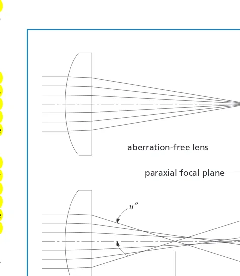
SPHERICAL ABERRATION
Figure 1.15 illustrates how an aberration-free lens focuses incoming collimated light. All rays pass through the focal point F″. The lower figure shows the situation more typically encountered in single lenses. The far-ther from the optical axis the ray enters the lens, the nearer to the lens it focuses (crosses the optical axis). The distance along the optical axis between the intercept of the rays that are nearly on the optical axis (paraxial rays) and the rays that go through the edge of the lens (marginal rays) is called longitudinal spherical aberration (LSA). The height at which these rays intercept the paraxial focal plane is called transverse spherical aberration (TSA). These quantities are related by
TSA =LSA#tan(u″).
Spherical aberration is dependent on lens shape, orientation, and conjugate ratio, as well as on the index of refraction of the materials present. Parameters for choosing the best lens shape and orientation for a given task are presented later in this chapter. However, the
third-TSA
longitudinal spherical aberration
transverse spherical aberration paraxial focal plane
F″
F″ u″
LSA aberration-free lens
Figure 1.15 Spherical aberration of a plano-convex lens
sinv1 v1 v1/ ! v / ! v / ! v / ! . . .
3 1 5
1 7
1 9
3 5 7 9
= − + − + − (1.21)
(1.22)
Gaussian
Beam Optics
Optical Specifications
Material Pr
operties
Optical Coatings
order, monochromatic, spherical aberration of a plano-convex lens used at infinite conjugate ratio can be estimated by
Theoretically, the simplest way to eliminate or reduce spherical aberration is to make the lens surface(s) with a varying radius of curvature (i.e., an aspheric surface) designed to exactly compensate for the fact that sin v≠v at larger angles. In practice, however, most lenses with high surface accuracy are manufactured by grinding and polishing techniques that naturally produce spherical or cylindrical surfaces. The manufacture of aspheric surfaces is more complex, and it is difficult to produce a lens of sufficient surface accuracy to eliminate spherical aberration completely. Fortunately, these aberrations can be virtually eliminated, for a chosen set of conditions, by combining the effects of two or more spherical (or cylindrical) surfaces.
In general, simple positive lenses have undercorrected spherical aberration, and negative lenses usually have overcorrected spherical aberration. By combining a positive lens made from low-index glass with a negative lens made from high-index glass, it is possible to produce a combination in which the spherical aberrations cancel but the focusing powers do not. The simplest examples of this are cemented doublets, such as the LAO series which produce minimal spherical aberration when properly used.
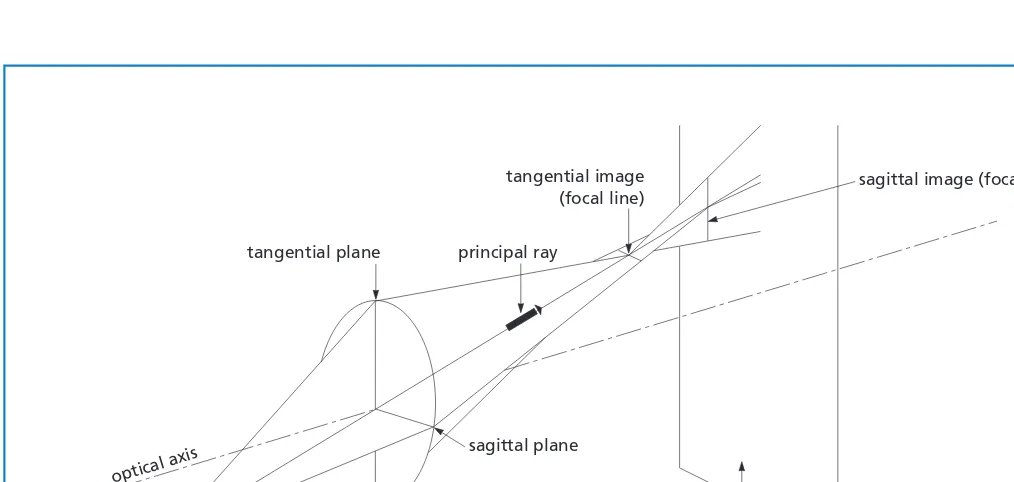
ASTIGMATISM
When an off-axis object is focused by a spherical lens, the natural asym-metry leads to astigmatism. The system appears to have two different focal lengths.
As shown in figure 1.16, the plane containing both optical axis and object point is called the tangential plane. Rays that lie in this plane are called tangential, or meridional, rays. Rays not in this plane are referred to as skew rays. The chief, or principal, ray goes from the object point through the center of the aperture of the lens system. The plane perpendicular to the tangential plane that contains the principal ray is called the sagittal or radial plane.
The figure illustrates that tangential rays from the object come to a focus closer to the lens than do rays in the sagittal plane. When the image is evaluated at the tangential conjugate, we see a line in the sagittal direction. A line in the tangential direction is formed at the sagittal conjugate. Between these conjugates, the image is either an elliptical or a circular blur. Astigmatism is defined as the separation of these conjugates.
The amount of astigmatism in a lens depends on lens shape only when there is an aperture in the system that is not in contact with the lens itself. (In all optical systems there is an aperture or stop, although in many cases it is simply the clear aperture of the lens element itself.) Astigmatism strongly depends on the conjugate ratio.
tangential image (focal line)
principal ray tangential plane
optical axis
object point
optical system sagittal plane
paraxial focal plane
sagittal image (focal line)
Figure 1.16 Astigmatism represented by sectional views
spot size due to spherical aberration f/# =0 0673
. .
f
Fundamental Optics
Gaussian Beam Optics
Optical Specifications
Material Pr
operties
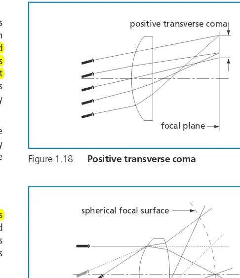
COMA
In spherical lenses, different parts of the lens surface exhibit different degrees of magnification. This gives rise to an aberration known as coma. As shown in figure 1.17, each concentric zone of a lens forms a ring-shaped image called a comatic circle. This causes blurring in the image plane (surface) of off-axis object points. An off-axis object point is not a sharp image point, but it appears as a characteristic comet-like flare. Even if spherical aberration is corrected and the lens brings all rays to a sharp focus on axis, a lens may still exhibit coma off axis. See figure 1.18.
As with spherical aberration, correction can be achieved by using multiple surfaces. Alternatively, a sharper image may be produced by judiciously placing an aperture, or stop, in an optical system to eliminate the more marginal rays.
FIELD CURVATURE
Even in the absence of astigmatism, there is a tendency of optical systems to image better on curved surfaces than on flat planes. This effect is called field curvature (see figure 1.19). In the presence of astigmatism, this problem is compounded because two separate astigmatic focal surfaces correspond to the tangential and sagittal conjugates.
Field curvature varies with the square of field angle or the square of image height. Therefore, by reducing the field angle by one-half, it is possible to reduce the blur from field curvature to a value of 0.25 of its original size.
Positive lens elements usually have inward curving fields, and negative lenses have outward curving fields. Field curvature can thus be corrected to some extent by combining positive and negative lens elements.
points on lens
1
1 2′ 0
3 3
4 2
4 2
1′
3′ 4′ 1′ 2′ 3′
4′
corresponding points on S
60∞ 1
2 4
3 1′
4′
3′ 2′ S
1
1 1′
S
P,O 1 1′
1′
Figure 1.17 Imaging an off-axis point source by a lens with positive transverse coma
positive transverse coma
focal plane
Figure 1.18 Positive transverse coma
spherical focal surface
Gaussian
Beam Optics
Optical Specifications
Material Pr
operties
Optical Coatings
DISTORTION
The image field not only may have curvature but may also be distorted. The image of an off-axis point may be formed at a location on this surface other than that predicted by the simple paraxial equations. This distor-tion is different from coma (where rays from an off-axis point fail to meet perfectly in the image plane). Distortion means that even if a perfect off-axis point image is formed, its location on the image plane is not correct. Furthermore, the amount of distortion usually increases with increasing image height. The effect of this can be seen as two different kinds of distortion: pincushion and barrel (see figure 1.20). Distortion does not lower system resolution; it simply means that the image shape does not correspond exactly to the shape of the object. Distortion is a sepa-ration of the actual image point from the paraxially predicted location on the image plane and can be expressed either as an absolute value or as a percentage of the paraxial image height.
It should be apparent that a lens or lens system has opposite types of distortion depending on whether it is used forward or backward. This means that if a lens were used to make a photograph, and then used in reverse to project it, there would be no distortion in the final screen image. Also, perfectly symmetrical optical systems at 1:1 magnification have no distortion or coma.
BARREL DISTORTION PINCUSHION
DISTORTION OBJECT
Figure 1.20 Pincushion and barrel distortion
white light ray
longitudinal chromatic aberration blue focal point
red focal point
red light ray blue light ray
Figure 1.21 Longitudinal chromatic aberration
Aperture Field Angle Image Height
Aberration (f) (v) (y)
Lateral Spherical f3 — —
Longitudinal Spherical f2 — —
Coma f2 v y
Astigmatism f v2 y2
Field Curvature f v2 y2
Distortion — v3 y3
Chromatic — — —
Variations of Aberrations with Aperture, Field Angle, and Image Height
CHROMATIC ABERRATION
Fundamental Optics
Gaussian Beam Optics
Optical Specifications
Material Pr
operties
LATERAL COLOR
Lateral color is the difference in image height between blue and red rays. Figure 1.22 shows the chief ray of an optical system consisting of a simple positive lens and a separate aperture. Because of the change in index with wavelength, blue light is refracted more strongly than red light, which is why rays intercept the image plane at different heights. Stated simply, magnification depends on color. Lateral color is very dependent on system stop location.
For many optical systems, the third-order term is all that may be needed to quantify aberrations. However, in highly corrected systems or in those having large apertures or a large angular field of view, third-order theory is inadequate. In these cases, exact ray tracing is absolutely essential.
aperture
red light ray lateral color
blue light ray
focal plane
Figure 1.22 Lateral Color
Achromatic Doublets Are Superior to
Simple Lenses
Because achromatic doublets correct for spherical as well as chromatic aberration, they are often superior to simple lenses for focusing collimated light or collimating point sources, even in purely monochromatic light.
Although there is no simple formula that can be used to estimate the spot size of a doublet, the tables in Spot Size give sample values that can be used to estimate the performance of catalog achromatic doublets.
Gaussian
Beam Optics
Optical Specifications
Material Pr
operties
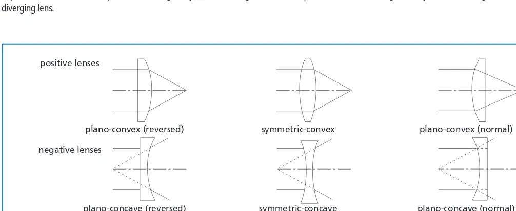
Optical Coatings
At infinite conjugate with a typical glass singlet, the plano-convex shape (q=1), with convex side toward the infinite conjugate, performs nearly as well as the best-form lens. Because a plano-convex lens costs much less to manufacture than an asymmetric biconvex singlet, these lenses are quite popular. Furthermore, this lens shape exhibits near-minimum total transverse aberration and near-zero coma when used off axis, thus enhancing its utility.
For imaging at unit magnification (s=s″ =2f), a similar analysis would show that a symmetric biconvex lens is the best shape. Not only is spherical aberration minimized, but coma, distortion, and lateral chro-matic aberration exactly cancel each other out. These results are true regardless of material index or wavelength, which explains the utility of symmetric convex lenses, as well as symmetrical optical systems in general. However, if a remote stop is present, these aberrations may not cancel each other quite as well.
For wide-field applications, the best-form shape is definitely not the optimum singlet shape, especially at the infinite conjugate ratio, since it yields maximum field curvature. The ideal shape is determined by the situation and may require rigorous ray-tracing analysis. It is possible to achieve much better correction in an optical system by using more than one element. The cases of an infinite conjugate ratio system and a unit conjugate ratio system are discussed in the following section.
Lens Shape
Aberrations described in the preceding section are highly dependent on application, lens shape, and material of the lens (or, more exactly, its index of refraction). The singlet shape that minimizes spherical aberration at a given conjugate ratio is called best-form. The criterion for best-form at any conjugate ratio is that the marginal rays are equally refracted at each of the lens/air interfaces. This minimizes the effect of sinv≠v. It is also the criterion for minimum surface-reflectance loss. Another benefit is that absolute coma is nearly minimized for best-form shape, at both infinite and unit conjugate ratios.
To further explore the dependence of aberrations on lens shape, it is helpful to make use of the Coddington shape factor, q, defined as
Figure 1.23 shows the transverse and longitudinal spherical aberrations of a singlet lens as a function of the shape factor, q. In this particular instance, the lens has a focal length of 100 mm, operates at f/5, has an index of refraction of 1.518722 (BK7 at the mercury green line, 546.1 nm), and is being operated at the infinite conjugate ratio. It is also assumed that the lens itself is the aperture stop. An asymmetric shape that corre-sponds to a q-value of about 0.7426 for this material and wavelength is the best singlet shape for on-axis imaging. It is important to note that the best-form shape is dependent on refractive index. For example, with a high-index material, such as silicon, the best-form lens for the infinite conjugate ratio is a meniscus shape.
SHAPE FACTOR (q) 42
ABERRA
TION
S
IN MILLIMETER
S
41.5 41 40.5 0 0.5 1 1.5 2
5
4
3
2
1
exact transverse spherical aberration (TSA)
exact longitudinal spherical aberration (LSA)
Figure 1.23 Aberrations of positive singlets at infinite conjugate ratio as a function of shape
q r r
r r
= +
−
( )
( ).
2 1
2 1
Fundamental Optics
Gaussian Beam Optics
Optical Specifications
Material Pr
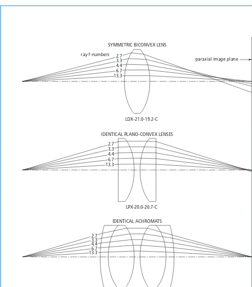
operties Previous examples indicate that an achromat is superior in performance to a singlet when used at the infinite conjugate ratio and at low f-numbers. Since the unit conjugate case can be thought of as two lenses, each working at the infinite conjugate ratio, the next step is to replace the plano-convex singlets with achromats, yielding a four-element system. The third part of figure 1.25 shows a system composed of two LAO-40.0-18.0 lenses. Once again, spherical aberration is not evident, even in the f/2.7 ray.
Lens Combinations
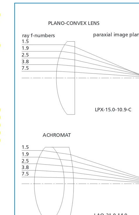
INFINITE CONJUGATE RATIO
As shown in the previous discussion, the best-form singlet lens for use at infinite conjugate ratios is generally nearly plano-convex. Figure 1.24 shows a plano-convex lens (LPX-15.0-10.9-C) with incoming collimated light at a wavelength of 546.1 nm. This drawing, including the rays traced through it, is shown to exact scale. The marginal ray (ray f-number 1.5) strikes the paraxial focal plane significantly off the optical axis.
This situation can be improved by using a two-element system. The second part of the figure shows a precision achromat (LAO-21.0-14.0), which consists of a positive low-index (crown glass) element cemented to a negative meniscus high-index (flint glass) element. This is drawn to the same scale as the plano-convex lens. No spherical aberration can be dis-cerned in the lens. Of course, not all of the rays pass exactly through the paraxial focal point; however, in this case, the departure is measured in micrometers, rather than in millimeters, as in the case of the plano-convex lens. Additionally, chromatic aberration (not shown) is much better corrected in the doublet. Even though these lenses are known as achromatic doublets, it is important to remember that even with monochromatic light the doublet’s performance is superior.
Figure 1.24 also shows the f-number at which singlet performance becomes unacceptable. The ray with f-number 7.5 practically intercepts the paraxial focal point, and the f/3.8 ray is fairly close. This useful drawing, which can be scaled to fit a plano-convex lens of any focal length, can be used to estimate the magnitude of its spherical aberration, although lens thickness affects results slightly.
UNIT CONJUGATE RATIO
Figure 1.25 shows three possible systems for use at the unit conjugate ratio. All are shown to the same scale and using the same ray f-numbers with a light wavelength of 546.1 nm. The first system is a symmetric biconvex lens (LDX-21.0-19.2-C), the best-form singlet in this application. Clearly, significant spherical aberration is present in this lens at f/2.7. Not until f/13.3 does the ray closely approach the paraxial focus.
A dramatic improvement in performance is gained by using two identical plano-convex lenses with convex surfaces facing and nearly in contact. Those shown in figure 1.25 are both LPX-20.0-20.7-C. The combination of these two lenses yields almost exactly the same focal length as the biconvex lens. To understand why this configuration improves performance so dramatically, consider that if the biconvex lens were split down the middle, we would have two identical plano-convex lenses, each working at an infinite conjugate ratio, but with the convex surface toward the focus. This orientation is opposite to that shown to be optimum for this shape lens. On the other hand, if these lenses are reversed, we have the system just described but with a better correction of the spherical aberration.
PLANO-CONVEX LENS
ray f-numbers
1.9 2.5 3.8 7.5 1.5
1.9 2.5 3.8 7.5 1.5
ACHROMAT
paraxial image plane
LPX-15.0-10.9-C
LAO-21.0-14.0
Gaussian
Beam Optics
Optical Specifications
Material Pr
operties
Optical Coatings
SYMMETRIC BICONVEX LENS
ray f-numbers
IDENTICAL PLANO-CONVEX LENSES
IDENTICAL ACHROMATS 2.7
3.3 4.4 6.7 13.3
2.7 3.3 4.4 6.7 13.3
2.7 3.3 4.4 6.7 13.3
paraxial image plane
LDX-21.0-19.2-C
LPX-20.0-20.7-C
LAO-40.0-18.0
Fundamental Optics
Gaussian Beam Optics
Optical Specifications
Material Pr
operties
CIRCULAR APERTURE
Fraunhofer diffraction at a circular aperture dictates the fundamental limits of performance for circular lenses. It is important to remember that the spot size, caused by diffraction, of a circular lens is
d=2.44l(f/#)
where dis the diameter of the focused spot produced from plane-wave illumination and lis the wavelength of light being focused. Notice that it is the f-number of the lens, not its absolute diameter, that determines this limiting spot size.
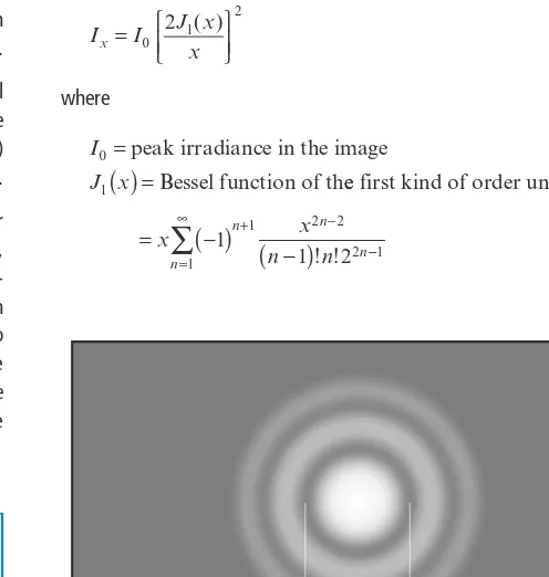
The diffraction pattern resulting from a uniformly illuminated circular aperture actually consists of a central bright region, known as the Airy disc (see figure 1.27), which is surrounded by a number of much fainter rings. Each ring is separated by a circle of zero intensity. The irradiance distribution in this pattern can be described by
where
Diffraction Effects
In all light beams, some energy is spread outside the region predicted by geometric propagation. This effect, known as diffraction, is a fundamental and inescapable physical phenomenon. Diffraction can be understood by considering the wave nature of light. Huygens’ principle (figure 1.26) states that each point on a propagating wavefront is an emitter of secondary wavelets. The propagating wave is then the envelope of these expanding wavelets. Interference between the secondary wavelets gives rise to a fringe pattern that rapidly decreases in intensity with increasing angle from the initial direction of propagation. Huygens’ principle nicely describes diffraction, but rigorous explanation demands a detailed study of wave theory.
Diffraction effects are traditionally classified into either Fresnel or Fraun-hofer types. Fresnel diffraction is primarily concerned with what happens to light in the immediate neighborhood of a diffracting object or aperture. It is thus only of concern when the illumination source is close to this aperture or object, known as the near field. Consequently, Fresnel diffraction is rarely important in most classical optical setups, but it becomes very important in such applications as digital optics, fiber optics, and near-field microscopy.
Fraunhofer diffraction, however, is often important even in simple optical systems. This is the light-spreading effect of an aperture when the aperture (or object) is illuminated with an infinite source (plane-wave illumination) and the light is sensed at an infinite distance (far-field) from this aperture.
From these overly simple definitions, one might assume that Fraunhofer diffraction is important only in optical systems with infinite conjugate, whereas Fresnel diffraction equations should be considered at finite conju-gate ratios. Not so. A lens or lens system of finite positive focal length with plane-wave input maps the far-field diffraction pattern of its aperture onto the focal plane; therefore, it is Fraunhofer diffraction that determines the limiting performance of optical systems. More generally, at any conjugate ratio, far-field angles are transformed into spatial displacements in the image plane.
aperture secondary wavelets
wavefront wavefront
some light diffracted into this region
AIRY DISC DIAMETER = 2.44 l f/#
Figure 1.27 Center of a typical diffraction pattern for a circular aperture
I I J x
x x= 0
1 2 2 ( ) ⎧ ⎩⎪
⎫
⎭⎪ (1.26)
I J x
0
1
=
( )
=peak irradiance in the image
Bessel function of thee first kind of order unity
=
( )
−−
(
)
=
∞ + −
∑
x x
n n
n
n n
n 1
1 2
1
1 2 2
2
! ! −−1
Gaussian
Beam Optics
Optical Specifications
Material Pr
operties
Optical Coatings
and
where
l=wavelength
D=aperture diameter
v=angular radius from the pattern maximum.
This useful formula shows the far-field irradiance distribution from a uniformly illuminated circular aperture of diameter D.
SLIT APERTURE
A slit aperture, which is mathematically simpler, is useful in relation to cylindrical optical elements. The irradiance distribution in the diffraction pattern of a uniformly illuminated slit aperture is described by
ENERGY DISTRIBUTION TABLE
The accompanying table shows the major features of pure (unaberrated) Fraunhofer diffraction patterns of circular and slit apertures. The table shows the position, relative intensity, and percentage of total pattern energy corresponding to each ring or band. It is especially convenient to characterize positions in either pattern with the same variable x. This
variable is related to field angle in the circular aperture case by
where Dis the aperture diameter. For a slit aperture, this relationship is given by
where wis the slit width, phas its usual meaning, and D, w, and lare all in the same units (preferably millimeters). Linear instead of angular field positions are simply found from r=s″tanvwhere s″is the secondary conjugate distance. This last result is often seen in a different form, namely the diffraction-limited spot-size equation, which, for a circular lens is
This value represents the smallest spot size that can be achieved by an optical system with a circular aperture of a given f-number, and it is the diameter of the first dark ring, where the intensity has dropped to zero.
The graph in figure 1.28 shows the form of both circular and slit aperture diffraction patterns when plotted on the same normalized scale. Aperture diameter is equal to slit width so that patterns between x-values and
angular deviations in the far-field are the same.
GAUSSIAN BEAMS
Apodization, or nonuniformity of aperture irradiance, alters diffraction patterns. If pupil irradiance is nonuniform, the formulas and results given previously do not apply. This is important to remember because most laser-based optical systems do not have uniform pupil irradiance. The out-put beam of a laser operating in the TEM00mode has a smooth Gaussian irradiance profile. Formulas used to determine the focused spot size from such a beam are discussed in Gaussian Beam Optics. Furthermore, when dealing with Gaussian beams, the location of the focused spot also departs from that predicted by the paraxial equations given in this chapter. This is also detailed in Gaussian Beam Optics.
Rayleigh Criterion
In imaging applications, spatial resolution is ultimately limited by diffraction. Calculating the maximum possible spatial resolution of an optical system requires an arbitrary definition of what is meant by resolving two features. In the Rayleigh criterion, it is assumed that two separate point sources can be resolved when the center of the Airy disc from one overlaps the first dark ring in the diffraction pattern of the second. In this case, the smallest resolvable distance, d, is
APPLICATION NOTE
d= 0.61 = l
NA 1.22 f/#
l
( )
I I x
x x= ⎧
⎩⎪ ⎫ ⎭⎪
0 2
sin (1.27)
I
x w
w 0=
=
= =
peak irradiance in image where
wavelength where
slit w
p v l l
sin
iidth
angular deviation from pattern maximum.
v=
sinv l
p
= x
D (1.28)
sinv l
p
= x
w (1.29)
d=2 44. fl
( )
/# (see eq. 1.25)x=pD
Fundamental Optics
Gaussian Beam Optics
Optical Specifications
Material Pr
operties
90.3% in central maximum
95.0% within the two adjoining subsidiary maxima POSITION IN IMAGE PLANE (x) CIRCULAR APERTURE
91.0% within first bright ring
83.9% in Airy disc
464544434241 47
48 0 1 2 3 4 5 6 7 8
0.0 .1 .2 .3 .4 .5 .6 .7 .8 .9 1.0
slit aperture
circular
aperture
NORMALIZED P
A
TTERN IRRADIAN
C
E (y)
Relative Energy Relative Energy
Position Intensity in Ring Position Intensity in Band
Ring or Band (x) (Ix/I0) (%) (x) (Ix/I0) (%)
Central Maximum 0.0 1.0 83.8 0.0 1.0 90.3
First Dark 1.22p 0.0 1.00p 0.0
First Bright 1.64p 0.0175 7.2 1.43p 0.0472 4.7
Second Dark 2.23p 0.0 2.00p 0.0
Second Bright 2.68p 0.0042 2.8 2.46p 0.0165 1.7
Third Dark 3.24p 0.0 3.00p 0.0
Third Bright 3.70p 0.0016 1.5 3.47p 0.0083 0.8
Fourth Dark 4.24p 0.0 4.00p 0.0
Fourth Bright 4.71p 0.0008 1.0 4.48p 0.0050 0.5
Fifth Dark 5.24p 0.0 5.00p 0.0
Slit Aperture Circular Aperture
Energy Distribution in the Diffraction Pattern of a Circular or Slit Aperture
limited, it is pointless to strive for better resolution. This level of resolution can be achieved easily with a plano-convex lens.
While angular divergence decreases with increasing focal length, spherical aberration of a plano-convex lens increases with increasing focal length. To determine the appropriate focal length, set the spherical aberration formula for a plano-convex lens equal to the source (spot) size:
This ensures a lens that meets the minimum performance needed. To select a focal length, make an arbitrary f-number choice. As can be seen from the relationship, as we lower the f-number (increase collection efficiency), we decrease the focal length, which will worsen the resultant divergence angle (minimum divergence =1 mm/f).
In this example, we will accept f/2 collection efficiency, which gives us a focal length of about 120 mm. For f/2 operation we would need a min-imum diameter of 60 mm. The LPX-60.0-62.2-C fits this specification exactly. Beam divergence would be about 8 mrad.
Finally, we need to verify that we are not operating below the theoretical diffraction limit. In this example, the numbers (1-mm spot size) indicate that we are not, since
diffraction-limited spot size =2.44#0.5 mm#2 =2.44 mm.
Example 2: Coupling an Incandescent Source into a Fiber
In Imaging Properties of Lens Systems we considered a system in which the output of an incandescent bulb with a filament of 1 mm in diameter was to be coupled into an optical fiber with a core diameter of 100 µm and a numerical aperture of 0.25. From the optical invariant and other constraints given in the problem, we determined that f=9.1 mm, CA =5 mm, s=100 mm, s″ =10 mm, NA″ =0.25, and NA =0.025 (or f/2 and f/20). The singlet lenses that match these specifications are the plano-convex LPX-5.0-5.2-C or biconvex lenses LDX-6.0-7.7-C and LDX-5.0-9.9-C. The closest achromat would be the LAO-10.0-6.0.
Gaussian
Beam Optics
Optical Specifications
Material Pr
operties
Optical Coatings
Lens Selection
Having discussed the most important factors that affect the performance of a lens or a lens system, we will now address the practical matter of selecting the optimum catalog components for a particular task. The fol-lowing useful relationships are important to keep in mind throughout the selection process:
$ Diffraction-limited spot size =2.44 lf/#
$ Approximate on-axis spot size
of a plano-convex lens at the infinite conjugate resulting from spherical aberration =
$ Optical invariant =
Example 1: Collimating an Incandescent Source
Produce a collimated beam from a quartz halogen bulb having a 1-mm-square filament. Collect the maximum amount of light possible and produce a beam with the lowest possible divergence angle.
This problem, illustrated in figure 1.29, involves the typical tradeoff between light-collection efficiency and resolution (where a beam is being collimated rather than focused, resolution is defined by beam diver-gence). To collect more light, it is necessary to work at a low f-number, but because of aberrations, higher resolution (lower divergence angle) will be achieved by working at a higher f-number.
In terms of resolution, the first thing to realize is that the minimum divergence angle (in radians) that can be achieved using any lens system is the source size divided by system focal length. An off-axis ray (from the edge of the source) entering the first principal point of the system exits the second principal point at the same angle. Therefore, increasing the system focal length improves this limiting divergence because the source appears smaller.
An optic that can produce a spot size of 1 mm when focusing a perfectly collimated beam is therefore required. Since source size is inherently
f
v min
v min = source size f
Figure 1.29 Collimating an incandescent source
0 067 1 3
.
/# .
f mm
f
=
0 067 3
. /# f
f
m=
″ NA
Fundamental Optics
Gaussian Beam Optics
Optical Specifications
Material Pr
operties
We can immediately reject the biconvex lenses because of spherical aberration. We can estimate the performance of the LPX-5.0-5.2-C on the focusing side by using our spherical aberration formula:
We will ignore, for the moment, that we are not working at the infinite conjugate.
This is slightly smaller than the 100-µm spot size we are trying to achieve. However, since we are not working at infinite conjugate, the spot size will be larger than that given by our simple calculation. This lens is therefore likely to be marginal in this situation, especially if we consider chromatic aberration. A better choice is the achromat. Although a computer ray trace would be required to determine its exact performance, it is virtually certain to provide adequate performance.
Example 3: Symmetric Fiber-to-Fiber Coupling
Couple an optical fiber with an 8-µm core and a 0.15 numerical aperture into another fiber with the same characteristics. Assume a wavelength of 0.5 µm.
This problem, illustrated in figure 1.30, is essentially a 1:1 imaging situation. We want to collect and focus at a numerical aperture of 0.15 or f/3.3, and we need a lens with an 8-µm spot size at this f-number. Based on the lens combination discussion in Lens Combination Formulas, our most likely setup is either a pair of identical plano-convex lenses or achromats, faced
front to front. To determine the necessary focal length for a plano-convex lens, we again use the spherical aberration estimate formula:
This formula yields a focal length of 4.3 mm and a minimum diameter of 1.3 mm. The LPX-4.2-2.3-BAK1 meets these criteria. The biggest problem with utilizing these tiny, short focal length lenses is the practical consid-erations of handling, mounting, and positioning them. Because using a pair of longer focal length singlets would result in unacceptable perfor-mance, the next step might be to use a pair of the slightly longer focal length, larger achromats, such as the LAO-10.0-6.0. The performance data, given in Spot Size, show that this combination does provide the required 8-mm spot diameter.
Because fairly small spot sizes are being considered here, it is important to make sure that the system is not being asked to work below the diffraction limit:
Since this is half the spot size caused by aberrations, it can be safely assumed that diffraction will not play a significant role here.
An entirely different approach to a fiber-coupling task such as this would be to use a pair of spherical ball lenses (LMS-LSFN series) or one of the gradient-index lenses (LGT series).
s = f s″= f
spot size=0 067 10 = m.
23 84
. ( )
m
0 067
3 33 0 008 .
. . mm.
f
=
. .
Gaussian
Beam Optics
Optical Specifications
Material Pr
operties
Optical Coatings
Example 4: Diffraction-Limited Performance
Determine at what f-number a plano-convex lens being used at an infinite conjugate ratio with 0.5-mm wavelength light becomes diffraction lim-ited (i.e., the effects of diffraction exceed those caused by aberration).
To solve this problem, set the equations for diffraction-limited spot size and third-order spherical aberration equal to each other. The result depends upon focal length, since aberrations scale with focal length, while diffraction is solely dependent upon f-number. By substituting some common focal lengths into this formula, we get f/8.6 at f=100 mm, f/7.2 at f=50 mm, and f/4.8 at f=10 mm.
When working with these focal lengths (and under the conditions previously stated), we can assume essentially diffraction-limited performance above these f-numbers. Keep in mind, however, that this treatment does not take into account manufacturing tolerances or chromatic aberration, which will be present in polychromatic applications.
2 44 0 5 0 067
54 9
3
1 4
. . /# .
/#
/# ( . ) ./
× × = ×
= ×
m f
f or
f
m f
f
Spherical Ball Lenses for Fiber Coupling
Spheres are arranged so that the fiber end is located at the focal point. The output from the first sphere is then collimated. If two spheres are aligned axially to each other, the beam will be transferred from one focal point to the other. Translational alignment sensitivity can be reduced by enlarging the beam. Slight negative defocusing of the ball can reduce the spherical aberration third-order contribution common to all coupling systems. Additional information can be found in “Lens Coupling in Fiber Optic Devices: Efficiency Limits,” by A. Nicia, Applied Optics, vol. 20, no. 18, pp 3136–45, 1981. Off-axis aberrations are absent since the fiber diameters are so much smaller than the coupler focal length.
APPLICATION NOTE
optical fiber
collimated light section
optical fiber LMS-LSFN coupling sphere LMS-LSFN
coupling sphere
uncoated
narrow band fb
Fundamental Optics
Gaussian Beam Optics
Optical Specifications
Material Pr
operties
The effect on spot size caused by spherical aberration is strongly dependent on f-number. For a plano-convex singlet, spherical aberration is inversely dependent on the cube of the f-number. For doublets, this relationship can be even higher. On the other hand, the spot size caused by diffraction increases linearly with f-number. Thus, for some lens types, spot size at first decreases and then increases with f-number, meaning that there is some optimum performance point at which both aberrations and diffraction combine to form a minimum.
Unfortunately, these results cannot be generalized to situations in which the lenses are used off axis. This is particularly true of the achromat/apla-natic meniscus lens combinations because their performance degrades rapidly off axis.
Spot Size
In general, the performance of a lens or lens system in a specific circumstance should be determined by an exact trigonometric ray trace. CVI Melles Griot applications engineers can supply ray-tracing data for particular lenses and systems of catalog components on request. In certain situations, however, some simple guidelines can be used for lens selection. The opti-mum working conditions for some of the lenses in this catalog have already been presented. The following tables give some quantitative results for a variety of simple and compound lens systems, which can be constructed from standard catalog optics.
In interpreting these tables, remember that these theoretical values obtained from computer ray tracing consider only the effects of ideal geometric optics. Effects of manufacturing tolerances have not been con-sidered. Furthermore, remember that using more than one element provides a higher degree of correction but makes alignment more difficult. When actually choosing a lens or a lens system, it is important to note the tolerances and specifications clearly described for each CVI Melles Griot lens in the product listings.
The tables give the diameter of the spot for a variety of lenses used at several different f-numbers. All the tables are for on-axis, uniformly illuminated, collimated input light at 546.1 nm. They assume that the lens is facing in the direction that produces a minimum spot size. When the spot size caused by aberrations is smaller or equal to the diffraction-limited spot size, the notation “DL” appears next to the entry. The shorter focal length lenses produce smaller spot sizes because aberrations increase linearly as a lens is scaled up.
f/# LDX-5.0-9.9-C LPX-8.0-5.2-C LAO-10.0-6.0
f/2 — 94 11
f/3 36 25 7
f/5 8 6.7 (DL) 6.7 (DL)
f/10 13.3 (DL) 13.3 (DL) 13.3 (DL)
Focal Length =10 mm
*Diffraction-limited performance is indicated by DL.
f/# LDX-50.0-60.0-C LPX-30.0-31.1-C LAO-60.0-30.0 LAO-100.0-31.5 & MENP-31.5-6.0-146.4-NSF8
f/2 816 600 — —
f/3 217 160 34 4 (DL)
f/5 45 33 10 6.7 (DL)
f/10 13.3 (DL) 13.3 (DL) 13.3 (DL) 13.3 (DL)
Spot Size (mm)* Spot Size (mm)*
Focal Length =60 mm
LAO-50.0-18.0 & f/# LPX-18.5-15.6-C LAO-30.0-12.5 MENP-18.0-4.0-73.5-NSF8
f/2 295 — 3
f/3 79 7 4 (DL)
f/5 17 6.7 (DL) 6.9 (DL)
f/10 13.3 (DL) 13.3 (DL) 13.8 (DL)
Focal Length =30 mm
Gaussian
Beam Optics
Optical Specifications
Material Pr
operties
Optical Coatings
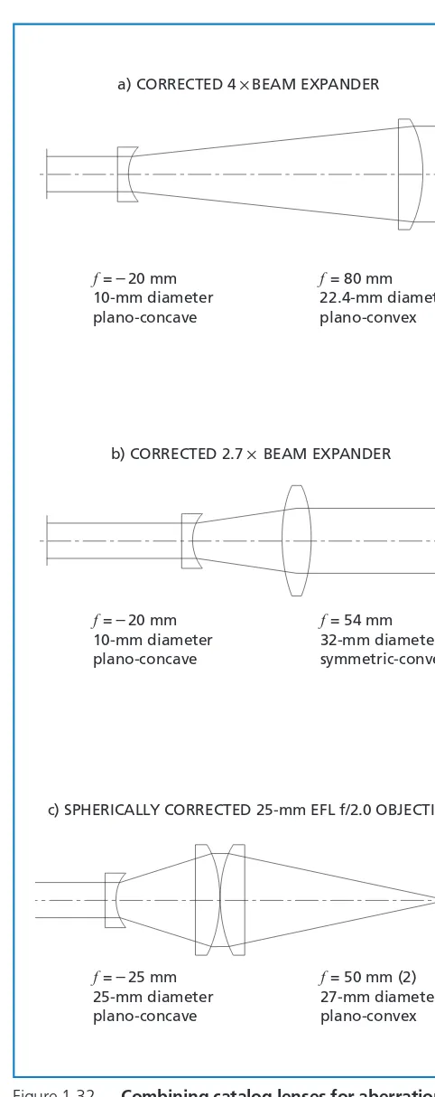
If a plano-convex lens of focal length f1oriented in the normal direction is combined with a plano-concave lens of focal length f2oriented in its reverse direction, the total spherical aberration of the system is
After setting this equation to zero, we obtain
To make the magnitude of aberration contributions of the two elements equal so they will cancel out, and thus correct the system, select the focal length of the positive element to be 3.93 times that of the negative element.
Figure 1.32(a) shows a beam-expander system made up of catalog elements, in which the focal length ratio is 4:1. This simple system is corrected to about 1/6 wavelength at 632.8 nm, even though the objective is operating at f/4 with a 20-mm aperture diameter. This is remarkably good wavefront correction for such a simple system; one would normally assume that a doublet objective would be needed and a complex diverging lens as well. This analysis does not take into account manufacturing tolerances.
A beam expander of lower magnification can also be derived from this information. If a