SHIFT-SHARE DESIGNS: THEORY AND INFERENCE
*Rodrigo Adão
Michal Kolesár
†Eduardo Morales
August 9, 2019
Abstract
We study inference in shift-share regression designs, such as when a regional outcome is re-gressed on a weighted average of sectoral shocks, using regional sector shares as weights. We conduct a placebo exercise in which we estimate the effect of a shift-share regressor constructed with randomly generated sectoral shocks on actual labor market outcomes across U.S. Commuting Zones. Tests based on commonly used standard errors with 5% nominal significance level reject the null of no effect in up to 55% of the placebo samples. We use a stylized economic model to show that this overrejection problem arises because regression residuals are correlated across regions with similar sectoral shares, independently of their geographic location. We derive novel inference methods that are valid under arbitrary cross-regional correlation in the regression residuals. We show using popular applications of shift-share designs that our methods may lead to substantially wider confidence intervals in practice.
JEL codes: C12, C21, C26, F16, F22
*We thank the editor, four anonymous referees, Kirill Borusyak, Peter Egger, Gordon Hanson, Bo Honoré, seminar
par-ticipants at Carleton University, CEMFI, Chicago Fed, EESP-FGV, Fed Board, GTDW, Johns Hopkins University, Princeton University, PUC-Rio, Stanford University, UC Irvine, Unil, University of Michigan, University of Nottingham, University of Virginia, University of Warwick, and Yale University, and conference participants at the CURE conference, CEPR-ERWIT conference, EIIT-FREIT, Globalization & Inequality BFI conference, NBER-ITI winter meeting, Sciences Po Summer Workshop, and Princeton-IES Workshop, for very useful comments and suggestions. We thank Juan Manuel Castro Vin-cenzi and Xiang Zhang for excellent research assistance. We thank David Autor, David Dorn and Gordon Hanson for sharing their code and data. All errors are our own.
†Corresponding author. 287 Julis Romo Rabinowitz Building, Princeton University, Princeton NJ 08544. Phone: (609)
1
Introduction
We study how to perform inference in shift-share designs: regression specifications in which one studies the impact of a set of shocks, or “shifters”, on units differentially exposed to them, with the exposure measured by a set of weights, or “shares”. Specifically, shift-share regressions have the form
Yi =βXi+Zi0δ+ei, where Xi = S
∑
s=1
wisXs, wis ≥0 for alls, and S
∑
s=1
wis ≤1. (1)
For example, in an investigation of the impact of sectoral demand shifters on regional employment changes, Yi is the change in employment in region i, the shifter Xs is a measure of the change in
demand for the good produced by sectors, and the share wis may be measured as the initial share of regioni’s employment in sectors. Other observed characteristics of regioniare captured by the vector
Zi, which includes the intercept, and ei is the regression residual. Shift-share specifications are
in-creasingly common in many contexts (see, e.g.,Bartik(1991),Blanchard and Katz(1992),Card(2001), orAutor, Dorn and Hanson(2013)). However, their formal properties are relatively understudied.
Our starting point is the observation that usual standard error formulas may substantially under-state the true variability of OLS estimators of βin eq. (1). We illustrate the importance of this issue through a placebo exercise. As outcomes, we use 2000–2007 changes in employment rates and average wages for 722 Commuting Zones in the United States. We build a shift-share regressor by combining actual sectoral employment shares in 1990 with randomly drawn sector-level shifters for 396 4-digit SIC manufacturing sectors. The placebo samples thus differ exclusively in the randomly drawn sec-toral shifters. For each sample, we compute the OLS estimate ofβin eq. (1) and test if its true value is zero. Since the shifters are randomly generated, their true effect is indeed zero. Valid 5% significance level tests should therefore reject the null of no effect in at most 5% of the placebo samples. We find, however, that usual standard errors—clustering on state as well as heteroskedasticity-robust errors— are much smaller than the standard deviation of the OLS estimator and, as a result, lead to severe overrejection. Depending on the labor market outcome used, the rejection rate for 5% level tests can be as high as 55% for heteroskedasticity-robust standard errors and 45% for standard errors clustered on state, and it is never below 16%.
To explain the source of this overrejection problem, we introduce a stylized economic model featuring multiple regions, each of which produces output in multiple sectors. The key ingredients of our model are a sector- and region-specific labor demand and a regional labor supply. We assume that labor demand in each sector-region pair has a sector-specific elasticity with respect to wages and an intercept that aggregates several sector-specific components (e.g. sectoral productivities and demand shifters for the corresponding sectoral good). Labor supply in each region is upward-sloping and has a region-specific intercept that may aggregate group-specific labor supply shifters (e.g. push factors that raise immigration from different countries of origin). Up to a first-order approximation, the impact of sector-level shocks on labor market outcomes takes the form of a shift-share specification similar to that in eq. (1).
A key insight of our model is that the regression residual ei in eq. (1) will generally account
wis that enter the construction of the regressor Xi, as well as shift-share components that aggregate
unobserved group-specific labor supply shifters using exposures ˜wig of regioni to group-g specific
shocks. Thus, the residual may incorporate multiple shift-share terms with shares correlated with those defining the shift-share regressorXi. Consequently, whenever two regions have similar shares,
they will not only have similar exposure to the shiftersXs, but will also tend to have similar values
of the residualsei. While traditional inference methods allow for some forms of dependence between
the residuals, such as spatial dependence within a state, they do not directly address the possible dependence between residuals generated by unobserved shift-share components. This is why, in our placebo exercise, traditional inference methods underestimate the variance of the OLS estimator ofβ, creating the overrejection problem.
We then establish the large-sample properties of the OLS estimator ofβin eq. (1) under repeated sampling of the shifters Xs, conditioning on the realized shares wis, controls Zi, and residuals ei.
This sampling approach is motivated by our economic model: we are interested in what would have happened to outcomes if the sector-level shocks Xs had taken different values, holding everything else constant. Our framework allows for heterogeneous effects of the shifters: one unit increase inXs
causes the outcome in regionito increase bywisβis, where βis is an unknown parameter.
Our key assumption is that, conditional on the controls and the shares, the shifters are as good as randomly assigned and independent across sectors. An advantage of this assumption is that it allows us to do inference conditionally onei; as a result, we can allow for anycorrelation structure
of the regression residuals across regions.1 In contrast, if, instead of assuming independence of the shifters across sectors, we modeled the correlation structure in the residual, as in the spatial econometrics literature (e.g.Conley,1999) or in the interactive fixed effects literature (e.g.Bai,2009; Gobillon and Magnac,2016), the resulting inference would be sensitive to the validity of the modeling assumptions. We show that the regression estimandβin eq. (1) corresponds to a weighted average of the heterogeneous parametersβis and derive novel confidence intervals that are valid in samples with
many regions and sectors. We also derive an analogous formula when Xi is used as an instrument
in an instrumental variables regression, which follows directly from the fact that the associated first-stage and reduced-form regressions take the form in eq. (1).
To gain intuition for our formula, it is useful to consider the special case in which each region is fully specialized in one sector (i.e. for everyi,wis =1 for some sectors). In this case, our procedure is
identical to using the usual clustered standard error formula, but with clusters defined as groups of regions specialized in the same sector. This is in line with the rule of thumb that one should “cluster” at the level of variation of the regressor of interest. In the general case, our standard error formula essentially forms sectoral clusters, the variance of which depends on the variance of a weighted sum of the regression residualsei, with weights that correspond to the shares wis.
We extend our baseline results in three ways. We provide versions of our standard errors that only require the shifters to be independent across “clusters” of sectors, allowing for arbitrary correlation
1This is similar to the insight inBarrios et al.(2012), who consider cross-section regressions estimated at an individual
among sectors belonging to the same “cluster.” We also show how to apply our framework to panel data settings in which we have multiple observations of each region over time. Finally, we cover applications in which the shifter is unobserved, but can be estimated using observable local shocks.
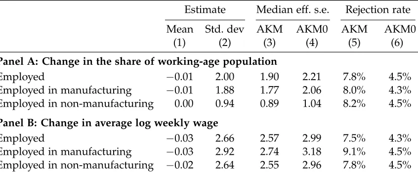
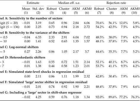
We illustrate the finite-sample properties of our novel inference procedure in the same placebo exercise that we use to show the bias of the usual standard error formulas. Our new formulas give a good approximation to the variability of the OLS estimator across the placebo samples; consequently, they yield rejection rates that are close to the nominal significance level. As predicted by the theory, our standard error formula remains accurate under alternative distributions of both the shifters and the regression residuals. When the number of sectors is small or there is a sector that is significantly larger than the rest, our method overrejects, although the overrejection is milder in comparison with the usual standard error formulas. If the shifters are not independent across sectors, we show that it is important to properly account for their correlation structure.
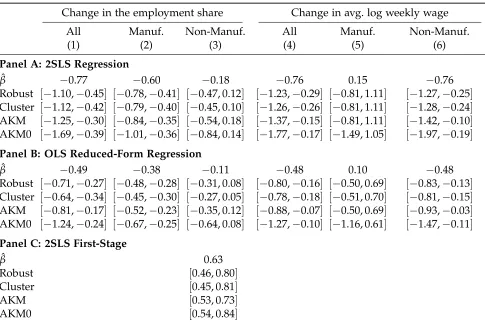
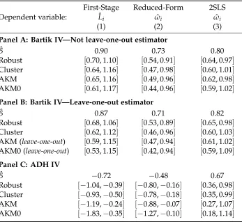
In the final part of the paper, we illustrate the implications of our new inference procedure for two popular applications of shift-share regressions. First, we study the effect of changes in sector-level Chinese import competition on labor market outcomes across U.S. Commuting Zones, as in Autor, Dorn and Hanson (2013). Second, we use changes in sector-level national employment to estimate the regional inverse labor supply elasticity, as inBartik(1991).2 Our new confidence intervals for the effects of Chinese competition on local labor markets increase by 23%–66% relative to those implied by state-clustered or heteroskedasticity-robust standard errors, although these effects remain statistically significant. In contrast, our confidence intervals for the inverse labor supply elasticity estimated using the procedure inBartik(1991) are very similar to those constructed using standard approaches.
Shift-share designs have been applied to estimate the effect of a wide range of shocks. For exam-ple, in seminal papers,Bartik(1991) andBlanchard and Katz(1992) use shift-share designs to analyze the impact on local labor markets of shifters measured as changes in national sectoral employment. More recently, shift-share strategies have been applied to investigate the local labor market impact of various shocks, including international trade competition (Topalova,2007,2010;Kovak,2013; Au-tor, Dorn and Hanson, 2013; Dix-Carneiro and Kovak, 2017; Pierce and Schott, 2018), credit supply (Greenstone, Mas and Nguyen,2015), technological change (Acemoglu and Restrepo,2019,2018), and industry reallocation (Chodorow-Reich and Wieland,2018). Shift-share regressors have been used as well to estimate the impact of immigration on labor markets, as in Card(2001) and many other pa-pers following his approach; see reviews in Lewis and Peri (2015) and Dustmann, Schönberg and Stuhler (2016). Furthermore, recent papers use shift-share strategies to estimate how firms respond to changes in outsourcing costs and foreign demand (Hummels et al.,2014;Aghion et al.,2018).3
Our paper is related to two other papers studying the statistical properties of shift-share instru-mental variables. First,Goldsmith-Pinkham, Sorkin and Swift(2018) consider using the full vector of
2Additionally, in Online Appendix F, we use changes in the stock of immigrants from various origin countries to
investigate the impact of immigration on employment and wages, followingAltonji and Card(1991) andCard(2001).
3Shift-share regressors have also been used to study the impact of sectoral shocks on political preferences (Autor et al.,
shares (wi1, . . . ,wiS)as an instrument for endogenous treatment. They conclude that this approach
requires the entire vector of shares to be as good as randomly assigned conditional on the shifters. Second,Borusyak, Hull and Jaravel(2018), focusing on the use of a shift-share regressor as an instru-ment, show it is a valid instrument if the set of shifters is as good as randomly assigned conditional on the shares, and discuss consistency of the instrumental variables estimator in this context. We follow Borusyak, Hull and Jaravel(2018) by modeling the shifters as randomly assigned, since this approach follows naturally from our economic model. Using this assumption, we point out the potential bias of standard inference procedures when applied to shift-share designs, and provide a novel inference procedure that is valid in this context.
While our paper focuses on the statistical properties of the OLS estimator of β in eq. (1), there exists a prior literature that has focused on studying the validity of different economic interpretations that one may attach to the estimandβ. For example, this prior literature has studied how this inter-pretation may be affected by the presence of cross-regional general equilibrium effects (Beraja, Hurst and Ospina, 2019; Adão, Arkolakis and Esposito,2019), slow adjustment of labor market outcomes to the shifters Xs (Jaeger, Ruist and Stuhler, 2018), and heterogeneous effects of the shifters across
sectors and regions (Monte, Redding and Rossi-Hansberg,2018).
The rest of this paper is organized as follows. Section 2 presents a placebo exercise illustrating the properties of the usual inference procedures. Section 3 introduces a stylized economic model and maps its implications into a potential outcome framework. Section4 establishes the asymptotic properties of the OLS estimator of βin eq. (1), as well as the properties of an instrumental variables estimator that uses a shift-share variable as an instrument. Section 5 discusses extensions of our baseline framework. Section6examines the performance of our novel inference procedures in a series of placebo exercises. Section 7 revisits two prior applications of shift-share designs, and Section 8 concludes. Proofs and additional results are collected in an Online Appendix.
2
Overrejection of usual standard errors: placebo evidence
In this section, we implement a placebo exercise to evaluate the finite-sample performance of the two inference methods most commonly applied in shift-share regression designs: (a) Eicker-Hubert-White—or heteroskedasticity-robust—standard errors, and (b) standard errors clustered on groups of regions geographically close to each other. In our placebo, we regress observed changes in U.S. regional labor market outcomes on a shift-share regressor that is constructed by combining actual data on initial sectoral employment shares for each region with randomly generated sector-level shocks. We describe the setup in Section2.1and discuss the results in Section2.2.
2.1 Setup and Data
We generate 30, 000 placebo samples indexed by m. Each of them contains N = 722 regions and
S= 396 sectors. We identify each regioniwith a U.S. Commuting Zone (CZ) and each sectors with a 4-digit SIC manufacturing industry.
in each placebo sample. The shares correspond to employment shares in 1990, and the outcomes correspond to changes in employment rates and average wages for different subsets of the population between 2000 and 2007. Our source of data on employment shares is the County Business Patterns, and our measures of changes in employment rates and average wages are based on data from the Census Integrated Public Use Micro Samples in 2000 and the American Community Survey for 2006 through 2008. Given these data sources, we construct our variables following the procedure described in the Online Appendix ofAutor, Dorn and Hanson(2013).
The placebo samples differ exclusively in the shifters {Xsm}N
s=1, which are drawn i.i.d. from a normal distribution with zero mean and variance equal to five in each placebo samplem. Since the shifters are independent of both the outcomes and the shares, the parameter β is zero; this is true irrespective of the dependence structure between the outcomes and the shares.
For each placebo sample m, given the observed outcome Yi, the generated shift-share regressor Xim and a vector of controls Zi including only an intercept, we compute the OLS estimate of β, the heteroskedasticity-robust standard error (which we labelRobust), and the standard error that clusters CZs in the same state (labeledCluster).
2.2 Results
Table1presents the median and standard deviation of the empirical distribution of the OLS estimates ofβacross the 30,000 placebo samples, along with the median standard error estimates, and rejection rates for 5% significance level tests of the null hypothesis H0: β = 0. We present these statistics for several outcome variables, which are listed in the leftmost column.
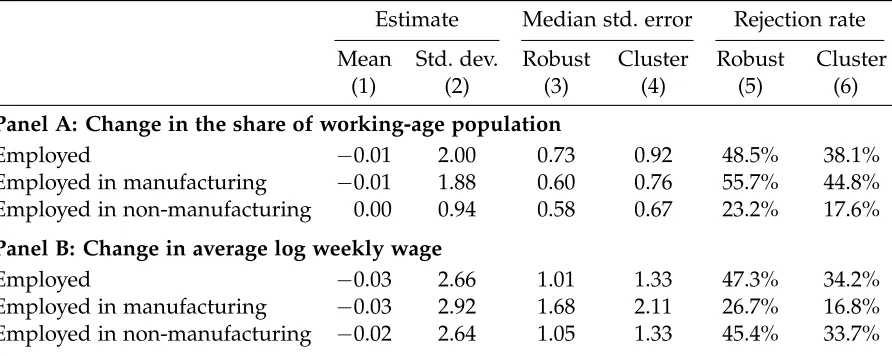
Column (1) of Table 1 shows that, up to simulation error, the average of the OLS estimates is zero for all outcomes. Column (2) reports the standard deviation of the estimated coefficients. This dispersion is the target of the estimators of the standard error of the OLS estimator.4 Columns (3) and (4) report the median standard error estimates for the Robust and Cluster procedures, respectively, and show that both standard error estimators are downward biased. On average across all outcomes, the median magnitudes of the heteroskedasticity-robust and state-clustered standard errors are, re-spectively, 55% and 46% lower than the standard deviation.
The downward bias in theRobustandClusterstandard errors translates into a severe overrejection of the null hypothesis H0: β = 0. Since the true value of β equals 0 by construction, a correctly behaved test with significance level 5% should have a 5% rejection rate. Columns (5) and (6) in Table1 show that traditional standard error estimators yield much higher rejection rates. For example, when the outcome variable is the CZ’s employment rate, the rejection rate is 48.5% and 38.1% whenRobust
and Cluster standard errors are used, respectively. These rejection rates are very similar when the dependent variable is instead the change in the average log weekly wage.
These results are quantitatively important. To see this, consider the following thought-experiment. Suppose we were to provide the 30, 000 simulated samples to 30, 000 researchers without disclosing the origin of the data to them. Instead, we would tell them that the shifters correspond to changes in a
4Figure D.1 in Online Appendix D.1 reports the empirical distribution of the OLS estimates when the dependent variable
Table 1: Standard errors and rejection rate of the hypothesis H0: β=0 at 5% significance level.
Estimate Median std. error Rejection rate
Mean Std. dev. Robust Cluster Robust Cluster
(1) (2) (3) (4) (5) (6)
Panel A: Change in the share of working-age population
Employed −0.01 2.00 0.73 0.92 48.5% 38.1%
Employed in manufacturing −0.01 1.88 0.60 0.76 55.7% 44.8%
Employed in non-manufacturing 0.00 0.94 0.58 0.67 23.2% 17.6%
Panel B: Change in average log weekly wage
Employed −0.03 2.66 1.01 1.33 47.3% 34.2%
Employed in manufacturing −0.03 2.92 1.68 2.11 26.7% 16.8%
Employed in non-manufacturing −0.02 2.64 1.05 1.33 45.4% 33.7%
Notes: For the outcome variable indicated in the leftmost column, this table indicates the mean and standard deviation of the OLS estimates ofβin eq. (1) across the placebo samples (columns (1) and (2)), the median standard error estimates
(columns (3) and (4)), and the percentage of placebo samples for which we reject the null hypothesisH0:β=0 using a 5%
significance level test (columns (5) and (6)). Robustis the Eicker-Huber-White standard error, andClusteris the standard error that clusters CZs in the same state. Results are based on 30,000 placebo samples.
sectoral shock of interest—for instance, trade flows, tariffs, or national employment. If the researchers set out to test the null that the impact of this shock is zero using standard inference procedures at a 5% significance level, then over a third of them would conclude that our computer generated shocks had a statistically significant effect on the evolution of employment rates between 2000 and 2007.
The following remark summarizes the results of our placebo exercise.
Remark 1. In shift-share regressions, traditional inference methods may suffer from a severe overrejection problem, and yield confidence intervals that are too short.
To understand the source of this overrejection problem, note that the standard error estimators reported in Table 1 assume that the regression residuals are either independent across all regions (forRobust), or between geographically defined groups of regions (for Cluster). Given that shift-share regressors are correlated across regions with similar employment shares {wis}Ss=1, these methods generally lead to a downward bias in the standard error estimate whenever regions with similar employment shares{wis}Ss=1 also have similar regression residuals. In the next section, we show how such correlations between regression residuals may arise.
3
Stylized economic model
describe the model fundamentals in Section3.1, discuss its main implications in Section3.2, and map these implications to a potential outcome framework in Section3.3.
3.1 Environment
We consider an economy with multiple sectors s = 1, . . . ,S and multiple regions i = 1, . . . ,N. We assume that the labor demand in sectorsand regioni, Lis, is given by
logLis = −σslogωi+logDis, σs >0, (2)
whereωi is the wage rate in regioni,σs is the labor demand elasticity in sectors, andDis is a
region-and sector-specific labor demregion-and shifter. This shifter may account for multiple sectoral components. Specifically, we decompose Dis into a sectoral shifter of interest χs, other shifters that vary by sector
µs, and a residual region- and sector-specific shifterηis:
logDis =ρslogχs+logµs+logηis. (3)
We assume that the labor supply in regioniis given by
logLi =φlogωi+logvi, φ>0, (4)
where φis the labor supply elasticity, and vi is a region-specific labor supply shifter. We allow this
shifter to have a shift-share structure that yields region-specific aggregates of group-specific labor supply shocks. In particular, indexing labor groups byg=1, . . . ,G, we decompose
logvi = G
∑
g=1 ˜
wiglogνg+logνi, (5)
where νg is a group-specific labor supply shifter, ˜wig measures the exposure of regioni to group g
labor supply shifter, and νi captures region-specific factors affecting labor supply. The variable νg
captures factors that affect the supply of labor of groupg in all regions in the population of interest. Workers may be classified into groups according to their education level, gender, or country of origin. We assume that workers cannot move across regions but are freely mobile across sectors. Thus, labor markets clear if
Li = S
∑
s=1
Lis, i=1, . . . ,N. (6)
3.2 Labor market equilibrium
We assume that, in each period, the model described by eqs. (2) to (6) characterizes the labor mar-ket equilibrium in every region, and that, across periods, changes in the labor marmar-ket outcomes
{ωi,Li}Ni=1 are due to changes in either the labor demand shifters,{χs,µs}Ss=1and{ηis}
N,S
We use ˆz = log(zt/z0) to denote log-changes in a variable z between a periodt = 0 and some other periodt. We assume that the realized changes between any two periods in all labor demand and supply shifters are draws from a joint distributionF(·):
{χˆs, ˆµs}Ss=1,{ηˆis}Ni=,1,Ss=1,{νˆg}gG=1{νˆi}iN=1
∼ F(·). (7)
Up to a first-order approximation around the initial equilibrium, eqs. (2) to (6) imply that the changes in employment and wages in regioniare given by
ˆ
Li = S
∑
s=1
lis0(θisχˆs+λiµˆs+λiηˆis) + (1−λi) ( G
∑
g=1 ˜
wigνˆg+νˆi), (8)
ˆ
ωi =φ−1
S
∑
s=1
l0is(θisχˆs+λiµˆs+λiηˆis)−φ−1λi( G
∑
g=1 ˜
wigνˆg+νˆi), (9)
where l0is = L0is/L0i is the initial employment share of sector s in region i, λi = φ
h
φ+∑Ss=1l0isσs i−1
, andθis =ρsλi.
Consider first the model’s implications for the impact on regional labor market outcomes of changes in sector-specific labor demand. We focus here on the impact of the demand shocks{χˆs, ˆµs}Ss=1 on the change in the employment rate ˆLi; however, given the symmetry between eqs. (8) and (9), the
model’s implications for the impact of these shocks on the change in the wage level ˆωi are analogous.
According to eq. (8), the change in the employment rate in region i depends on two shift-share components that aggregate the impact of the sector-specific labor demand shocks. In both compo-nents, the “share” term is the initial employment share l0is; the “shift” term corresponds in each of them to one of the two sector-specific labor demand shocks, ˆχs or ˆµs. Furthermore, ˆLi also depends
on additional shift-share terms that aggregate the impact of group-specific labor supply shocks. In this case, the “share” term is the region’s exposure to each group-specific shock, ˜wig. Conditional on
a sectors and a labor groupg, the shares{l0
is}iN=1and{w˜ig}iN=1 may be correlated. Settings in which the outcome of interest depends on multiple shift-share terms with potentially correlated shares is central to understanding the placebo results presented in Section2.
Another implication of eq. (8) is that, even conditional on the initial employment share l0
is, the
impact of sectoral labor demand shocks on regional employment may be heterogeneous across sectors and regions; e.g., the impact of ˆχson ˆLi depends not only onl0isbut also onθis, which may vary across iands. While datasets usually contain information on the initial employment shares for every sector and region{lis0}Ni=,S1,s=1, the parameters{θis}iN=,S1,s=1are not generally known.
We summarize the discussion in the last two paragraphs in the following remark:
Remark 2. In our model, the equilibrium equations for the change in regional labor market outcomes combines multiple shift-share terms, and the shifter effects depend on unknown parameters that may be heterogeneous.
interpre-tation of the different terms entering the labor demand shifter Dis in eq. (3).5 In addition, Online
Appendix C.3 shows that similar insights arise in a model that allows for migration across regions. In this case, the change in regional employment depends not only on the region’s own shift-share terms included in eq. (8), but also on a component, common to all regions, that combines the shift-share terms corresponding to all N regions. In this environment,l0isθis is the partial effect of the shifter ˆχs
on ˆLi conditional on a fixed effect that absorbs cross-regional spillovers created by migration.
Turning to the estimation of the inverse labor supply elasticity, eqs. (4) and (5) imply that
ˆ
ωi =φ˜Lˆi−φ˜(
G
∑
g=1 ˜
wigνˆg+νˆi) with φ˜ =φ−1. (10)
It follows from eq. (8) that the change in region i’s employment rate, ˆLi, also depends on the term
∑G
g=1w˜igνˆg+νˆi. Thus, the two terms on the right-hand side of eq. (10) are correlated with each other,
creating an endogeneity problem. The instrumental variables solution to this problem relies on the observation that using eqs. (8) and (9), one can write the inverse labor supply elasticity as the ratio of the impact of a sector-specific labor demand shock (e.g. ˆχs) on wages to that on employment:
˜ φ= ∂ωˆi
∂χˆs
∂Lˆi
∂χˆs
.
In Sections 4 and 5, we use the model described here to provide an economic interpretation for the econometric assumptions we impose when discussing identification and estimation in shift-share designs. These assumptions imply restrictions on the distribution of labor supply and demand shocks
F(·)introduced in eq. (7). In Section7, we return to this economic model when interpreting empirical estimates of the impact of sector-specific labor demand shifters on regional labor market outcomes (Section7.1); and the regional inverse labor supply elasticity (Section7.2).
3.3 From economic model’s equilibrium conditions to a potential outcome framework
We build on the results in Section3.2to propose a general framework for the estimation of the impact of shifters on outcomes measured at a different unit of observation. For concreteness, we refer to the level at which shifters vary as sectors and to the level at which the outcome varies as regions.
To make precise what we mean by “the effect of shifters on an outcome”, we use the potential outcomes notation, writingYi(x1, . . . ,xS)to denote the potential (counterfactual) outcome that would
occur in region i if the shocks to the S sectors were exogenously set to {xs}Ss=1. Consistently with eqs. (8) and (9), we assume that the potential outcomes are linear in the shocks,
Yi(x1, . . . ,xS) =Yi(0) + S
∑
i=1
wisxsβis, where wis ≥0 for alls, S
∑
s=1
wis ≤1, (11)
5In Online Appendix B, we derive eqs. (8) and (9) from a multisector gravity model with endogenous labor supply that
andYi(0) = Yi(0, . . . , 0)denotes the potential outcome in regioniwhen all shocks {xs}Ss=1 are set to zero. Thus, increasingxs by one unit, holding the shocks to the other sectors constant, leads to an
increase in regioni’s outcome ofwisβis units. This is the treatment effect ofxs onYi(x1, . . . ,xS). The
actual (observed) outcome is given by Yi = Yi(X1, . . . ,XS), which depends on the realization of the
shifters,(X1, . . . ,XS).
If the shifters of interest are the sectoral labor demand shocks{χˆs}Ss=1, and the outcome of interest is the employment change ˆLi, we can map eq. (8) into eq. (11) by defining
Yi =Lˆi, wis =l0is, xs=χˆs, βis = θis, Yi(0) =λi S
∑
s=1
wis(µˆs+ηˆis) + (1−λi)( G
∑
g=1 ˜
wigνˆg+υˆi). (12)
Observe thatYi(0)aggregates all shifters other than the sectoral shocks of interest{χˆs}Ss=1.6
We are interested in the properties of the OLS estimator ˆβ of the coefficient on the shift-share regressor Xi = ∑Ss=1wisXs in a regression of Yi onto Xi.7 To focus on the key conceptual issues, we
abstract away from any additional covariates or controls for now, and assume that Xs and Yi have
been demeaned, so that we can omit the intercept in a regression ofYi on Xi (see Section4.2for the
case with controls). In this simplified setting, the OLS estimator of the coefficient onXi is given by
ˆ β= ∑
N i=1XiYi
∑N i=1X2i
, (13)
and we can write the regression equation as
Yi = βXi+ei, where Xi = S
∑
s=1
wisXs. (14)
The definition of the estimand β in eq. (14) and the properties of the estimator ˆβ will depend on: (a) what is the population of interest; and (b) how we think about repeated sampling. For (a), we define the population of interest to be the observed set ofN regions, as opposed to focusing on a large superpopulation of regions from which theNobserved regions are drawn. Consequently, we are interested in the parameters {βis}iN=,S1,s=1 and the treatment effects {wisβis}Ni=,S1,s=1 themselves, rather than the distributions from which they are drawn, which would be the case if we were interested in a superpopulation of regions.8 For (b), given our interest on estimating theceteris paribusimpact of a specific set of shocks(X1, . . . ,XS), we consider repeated sampling of these shocks, while holding the shares{wis}iN=,S1,s=1, the parameters{βis}
N,S
i=1,s=1, and the potential outcomes{Yi(0)}iN=1fixed.
6Given the mapping in eq. (12), the expression in eq. (11) captures the first-order impact of the labor demand shocks
{χˆs}Ss=1 on changes in the employment rate. We focus on this first-order impact because it helps connecting our analysis
to linear specifications used extensively in the shift-share literature. See Online Appendix D.5 for a discussion of the approximation error arising from the linear specification imposed in eq. (8).
7We assume for now that the shifters{X
s}Ss=1 are directly observable. In Section5.3, we consider the case in which we
only observe noisy estimates of these shifters.
8Treating the set of observed regions as the population of interest is common in applications of the shift-share approach.
Given these assumptions, the estimand β is defined as the population analog of eq. (13) under repeated sampling of the shocksXs,
β= ∑
N
i=1E[XiYi |F0] ∑N
i=1E[Xi2|F0]
, with F0 ={Yi(0),βis,wis}iN=,S1,s=1, (15)
and, given eqs. (11) and (14), the regression errorei is then defined as the residual
ei =Yi−Xiβ=Yi(0) + S
∑
i=1
wisXs(βis−β). (16)
Thus, the statistical properties of the regression residual ei depend on the properties of the
po-tential outcome Yi(0), the shifters {Xs}sS=1, the shares {wis}Ss=1, and the difference between the pa-rameters{βis}Ss=1 and the estimand β. Importantly, as illustrated in eq. (12), the potential outcome
Yi(0) will generally incorporate terms that have a shift-share structure with shares that are either
identical to (e.g. the term∑Ss=1wisµˆs) or different from but potentially correlated with (e.g. the term
∑G
g=1w˜igνˆg) the shares{wis}Ss=1 that define the shift-share regressor Xi. It then follows from eq. (16) that the residualsei and ei0 will generally be correlated for any pair of regionsi andi0 with similar
values of the shift-share regressor.
We summarize this discussion in the following remark.
Remark 3. Correct inference for the coefficient on a shift-share regressor requires taking into account potential cross-regional correlation in residuals across observations with similar values of the shift-share covariate of interest. One possible source of such correlation is the presence in these residuals of shift-share components with shares identical to or correlated with those entering the covariate of interest.
Remark 3 has important implications for estimating the sampling variability of ˆβ. In particular, traditional inference procedures do not account for correlation ineiamong regions with similar shares
and, therefore, tend to underestimate the variability of ˆβ. As we formalize in the next section, this is the main reason for the overrejection problem described in Section2.
4
Asymptotic properties of shift-share regressions
In this section, we formulate the statistical assumptions that we impose on the data generating pro-cess (DGP), use them to derive asymptotic results, and provide an economic interpretation of these assumptions using the model introduced in Section 3. In Section4.1, we consider the case in which there is a single shift-share regressor and no controls. We account for controls in Section4.2. In Sec-tion4.3, we consider using the shift-share variable as an instrument for a regional treatment variable. All proofs and technical details are collected in Online Appendix A.
We follow the notation from eq. (1) by writing sector-level variables (such as the shifter Xs) in
script font style and region-level aggregates (such asXi) in normal style. We use standard matrix and vector notation. In particular, for a (column) L-vector Ai that varies at the regional level, A denotes
denotes theS×L matrix with thesth row given byAs0. If L= 1, thenAandA are an N-vector and anS-vector, respectively. Let W denote theN×Smatrix of shares, so that its(i,s)element is given bywis, and letBdenote the N×Smatrix with(i,s)element given byβis.
4.1 Simple case without controls
We focus here on the statistical properties of the OLS estimator ˆβdefined in eq. (13).
Assumptions
We consider large-sample properties of ˆβas the number sectors goes to infinity, S→∞. The assump-tions below imply that N → ∞ as S → ∞. To assess how large S needs to be in order that these asymptotics provide a good approximation to the finite sample distribution of ˆβ, we conduct a series of placebo simulations in Section6. We describe here the main substantive assumptions, and collect technical regularity conditions in Online Appendix A.1.1. As in eq. (15), letF0 = (Y(0),B,W).
Assumption 1(Identification). (i) The observed outcome is given byYi = Yi(X1, . . . ,XS), such that
eq. (11) holds; (ii) The shifters are as good as randomly assigned conditional onF0in the sense that, for alls=1, . . . ,S,
E[Xs|F0] =0. (17)
Assumption 1(i) requires that the potential outcomes are linear in the shifters {Xs}Ss=1. As dis-cussed in Section3.3, one can generate such linear specification from a first-order approximation of the impact of the shifters (X1, . . . ,XS) on the outcome Yi. This approximation may be subject to
error. In Online Appendix A.1.1, we generalize eq. (11) to allow for a linearization error and derive restrictions on this error under which our inference procedures remain valid.
Assumption 1(ii) imposes that the sectoral shifters X are mean independent of the shares W, potential outcomes Y(0), and parameters B; the assumption that the shifters are mean zero is a normalization to allow us to drop the intercept; we relax it in Section4.2. This random assignment assumption is a key assumption for identifying the causal impact of a shift-share covariate; a version of this assumption has been previously proposed byBorusyak, Hull and Jaravel(2018).
If we are interested in studying the effect of labor demand shifters in the context of the model in Section3 (i.e. Xs = χˆs), Assumption1(ii)will hold if the shifters {χˆs}Ss=1 are mean independent of the other labor demand shifters, {µˆs}Ss=1 and {ηˆis}
N,S
i=1,s=1, and of the labor supply shifters, {νˆg}Gg=1 and {νˆi}iN=1. The plausibility of this restriction depends on the specific empirical application. For example, if allNregions in the sample are regions within a small open economy, ˆχsdenotes changes
in international prices in sectors, and ˆµs denotes changes in the tariffs that this small open economy
charges on its sector s imports; then, Assumption1(ii) requires these changes in tariffs to be inde-pendent of the changes in tariffs in any country that is large enough for their tariff changes to affect international prices (see Online Appendix B.4 for additional details).
Assumption 2(Consistency and Inference). (i) The shifters(X1, . . . ,XS)are independent conditional
on F0; (ii) maxsns/∑St=1nt → 0, where ns = ∑Ss=1wis denotes the total share of sector s; (iii)
Assumption 2(i)requires the shifters to be independent. It adapts to our setting the assumption underlying randomization-style inference in randomized controlled trials that the treatment assign-ment is independent across entities (see Imbens and Rubin, 2015, for a review). An independence or a weak dependence assumption of this type is generally necessary in order to do inference.9 One
could alternatively impose assumptions on the correlation structure of the regression residuals, ei-ther by imposing a particular structure on them, as in the literature on interactive fixed effects (e.g. Gobillon and Magnac, 2016), or by imposing a distance metric on the observations, as in the spatial econometrics literature (e.g.Conley,1999). However, as the economic model in Section3 shows, the structure of the residuals may be very complex. The residuals may include potentially correlated region-specific terms as well as several shift-share terms, which may or may not use the same shares as the covariate of interestXi. It is thus difficult to conceptualize which exact restriction on their joint
distribution one should impose.
By instead imposing restrictions on the distribution of the vector of shifters (X1, . . . ,XS)
con-ditional on F0 = (Y(0),B,W), Assumption 2(i) ensures that the standard errors we derive remain valid underanydependence structure between the shareswis across sectors and regions, and under anycorrelation structure of the potential outcomes Yi(0)or, equivalently, of the regression errors ei,
across regions.10 We thus do not have to worry about correctly specifying this correlation structure, as one would under the alternative approaches mentioned above. Our approach allows (but does not require) the residual to have a shift-share structure; it similarly allows all{wis}Ni=,S1,s=1 to be equi-librium objects responding to the same economic shocks, and thus be correlated across regions and sectors.11 In Section5.1, we relax Assumption2(i)and allow for a non-zero correlation in the shifters
(X1, . . . ,XS)within clusters of sectors; we only require that the shifters are independent across the
clusters. Additionally, in the context of the empirical application in Section7.1, we discuss how to perform inference in a setting in which all shifters of interest are generated by a common shock that has heterogeneous effects across sectors.
In the economic model in Section 3, if Xs = χˆs and we interpret these shocks as, for example,
sector-specific productivity shocks, Assumption 2(i) requires that there is no common component driving the changes in sectoral productivities. Our approach does not require the shifters{Xs}Ss=1 to be identically distributed; we allow, for example, the variance of the shock to differ across sectors.
Assumptions 2(ii)and2(iii)are our main regularity conditions.12 Assumption2(ii)is needed for
9For example, for inference on average treatment effects, which is commonly the goal when running a regression, one
typically assumes that the sample is a random sample from the population of interest and, thus, that the treatment variable is independent across the individuals in the sample.
10Since our inference is valid conditional on{
ei}Ni=1, it accounts for any correlation structure they may have, including
spatial, or, in applications with multiple periods, temporal correlations. See Section5.2for settings with multiple periods.
11This conceptualization of all the sharesw
isas equilibrium objects that respond (at least partly) to the same set of shocks
is consistent with the model in Section3. As shown in eq. (12), each sharewis corresponds to the share of workers in
regioniemployed in sectorsin an initial equilibrium,l0
is. Furthermore, each of these initial employment shares will be a
function of the same sector-specific demand shocks and group-specific labor supply shocks; consequentlyl0iswill generally be correlated withl0
i0s0 even fori6=i0ands6=s0.
12In the context of a shift-share instrumental variables regression,Goldsmith-Pinkham, Sorkin and Swift(2018) discuss
similar conditions stated in terms of Rotemberg weights. This is convenient under the baseline assumption considered in Goldsmith-Pinkham, Sorkin and Swift(2018) that the vector of shares(wi1, . . . ,wiS)is exogenous, because the Rotemberg
consistency: it requires that the size of each sector,ns, is asymptotically negligible. This assumption
is analogous to the standard consistency condition in the clustering literature that the largest cluster be asymptotically negligible. To see the connection, consider the special case with “concentrated sectors”, in which each region i specializes in one sector s(i); i.e. wis = 1 if s = s(i) and wis = 0
otherwise, andnsis thus the number of regions that specialize in sectors. In this case,Xi =Xs(i), so
that, if eq. (17) holds, ˆβis equivalent to an OLS estimator in a randomized controlled trial in which the treatment varies at a cluster level; here thesth cluster consists of regions that specialize in sector
s. The condition maxsns/∑St=1nt → 0 then reduces to the assumption that the largest cluster be
asymptotically negligible. Assumption2(iii) is needed for asymptotic normality—it ensures that the Lindeberg condition holds. It strengthens Assumption2(ii)slightly by requiring that the contribution of each sector to the asymptotic variance is asymptotically negligible; otherwise the estimator will not generally be asymptotically normal, even if it is consistent.
In terms of the economic model introduced in Section3, Assumptions2(ii)and2(iii) require that no sector dominates the rest in terms of initial employment at the national level; i.e. ∑Ni=1l0is is not too
large for any sector. Section6.1shows that this assumption is reasonable for the U.S. if theSsectors used to construct the treatment of interestXi correspond to the 396 4-digit manufacturing sectors (see
Section2.1). In Section6.2, we illustrate the consequences of the failure of this assumption due to the inclusion of a large aggregate sector, the non-manufacturing sector, inXi.
Asymptotic theory
We now establish that the OLS estimator in eq. (13) is consistent and asymptotically normal.
Proposition 1. Suppose Assumption 1, Assumptions 2(i) and 2(ii), and Assumptions A.1(i) to A.1(iii) in Online Appendix A.1.1 hold. Then
β= ∑
N
i=1∑Ss=1πisβis
∑N
i=1∑Ss=1πis
, and βˆ =β+op(1), (18)
whereπis =w2isvar(Xs|F0).
This proposition gives two results. First, it shows that the estimand βin eq. (15) can be expressed as a weighted average of the region- and sector-specific parameters {βis}iN=,S1,s=1, with the weight πis
increasing in the sharewisand in the conditional variance of the shifter var(Xs|F0). Second, it states that the OLS estimator ˆβconverges to this estimand as S → ∞. The special case with concentrated sectors is again useful in interpreting Proposition1. In this case, ∑Ss=1πisβis = var(Xs(i) | F0)βis(i)
and, therefore, the first result in Proposition 1 reduces to the standard result from the randomized controlled trials literature with cluster-level randomization (with each “cluster” defined as all regions specialized in the same sector) that the weights are proportional to the variance of the shock.
sector-specific weights{ξis}iN=,S1,s=1, yields the weighted average treatment effect
τξ =
∑N
i=1∑Ss=1ξiswisβis
∑N
i=1∑Ss=1ξis
.
Alternatively, the total effect of increasing the shifters simultaneously in every sector by one unit is ∑Ss=1wisβis; weighting it using a set of region-specific weights {ζi}iN=1 yields the weighted to-tal treatment effect τζT = ∑Ni=1ζi∑Ss=1wisβis/∑iN=1ζi. If βis is constant across i and s, then β = τζT, provided ∑Ss=1wis = 1 in every region i; otherwise, we can consistently estimate τζT by ˆβ· ∑N
i=1ζi∑Ss=1wis/∑iN=1ζi. Similarly, if βis is constant across i and s, τξ is consistently estimated by
ˆ
β·∑iN=1∑Ss=1ξiswis/∑Ni=1∑Ss=1ξis. On the other hand, if βis varies across regions and sectors, then
it is not clear in general how to exploit knowledge of the estimand β defined in eq. (18) to learn something aboutτξ orτζT. A special case in which it is possible to consistently estimateτξ even ifβis
varies acrossior s arises whenXs is homoskedastic, var(Xs |F0) = σ2, and ξis = wis; in this case, a
consistent estimate ofτξ is given by ˆβ∑
N
i=1∑Ss=1w2is/∑Ni=1∑Ss=1wis.13
Proposition 2. Suppose Assumptions1and2, and Assumption A.1 in Online Appendix A.1.1 hold. Suppose also that
VN = 1
∑S s=1n2s
var
N
∑
i=1
Xiei |F0
!
converges in probability to a non-random limit. Then
N q
∑S s=1n2s
(βˆ−β) =N
0, VN 1
N ∑Ni=1X2i 2
+op(1).
This proposition shows that ˆβ is asymptotically normal, with a rate of convergence equal to
N(∑Ss=1n2s)−1/2. If all sector sizesnsare of the order N/S, the rate of convergence equals
√
S. How-ever, if the sizes are unequal, the rate may be slower.
According to Proposition2, the asymptotic variance formula has the usual “sandwich” form. Since
Xi is observed, to construct a consistent standard error estimate, it suffices to construct a consistent
estimate ofVN, the middle part of the sandwich. To motivate our standard error formula, suppose
that βis is constant acrossiands,βis =β. Then it follows from eq. (17) and Assumption2(i)that
VN = ∑ S
s=1var(Xs |F0)R2s
∑S s=1n2s
, Rs=
N
∑
i=1
wisei. (19)
13In general, one can consistently estimateτ
ξ orτ
T
Replacing var(Xs|F0)byXs2, andei by the regression residual ˆei =Yi−Xiβˆ, we obtain the estimate
b
VAKM(βˆ) = ˆ
VAKM(βˆ)
∑N i=1X2i
2,
ˆ
VAKM(βˆ) =
S
∑
s=1
Xs2Rˆ2s, Rˆs= N
∑
i=1
wiseˆi. (20)
Whenβis = β, we show formally that this variance estimate leads to valid inference under regularity conditions in Section4.2. In Online Appendix A.1.6 we show that this variance estimate remains valid under heterogeneousβis under further regularity conditions.
To gain intuition for the variance estimate in eq. (20), consider the case with concentrated sectors. Then the numerator in eq. (20) becomes ∑Ss=1Xs2Rˆ2
s = ∑Ss=1(∑iN=1I{s(i) = s}Xieˆi)2, so that eq. (20)
reduces to the cluster-robust variance estimate that clusters on the sector that each region is special-ized. This is consistent with the rule of thumb that one should “cluster” at the level of variation of the regressor of interest. More generally, the variance estimate essentially forms sectoral clusters with variance that depends on the variance of ˆRs, a weighted sum of the regression residuals{eˆi}Ni=1, with weights that correspond to the shares{wis}iN=1. An important advantage ofVbAKM(βˆ)is that it allows
for an arbitrary structure of cross-regional correlation in residuals:
Remark 4. In the expression forVN in eq.(19), the expectation is only taken over{Xs}Ss=1—we do not take any
expectation over the shares{wis}iN=,S1,s=1or the residuals{ei}Ni=1. This is because our inference is conditional on
the realized values of the shares and on the potential outcomes{Yi(0)}N
i=1. In terms of the regression in eq.(14),
this means that we consider properties of βˆ under repeated sampling of Xi = ∑Ss=1wisXs conditional on the shares{wis}iN=,S1,s=1and on the residuals{ei}iN=1(as opposed to, say, considering properties ofβˆunder repeated
sampling of the residuals conditional on {Xi}N
i=1). As a result, our inference method allows for arbitrary
dependence between the residuals{ei}Ni=1.
To understand the source of the overrejection problem discussed in Section2, let us compare the variance estimateVbAKM(β) with the cluster-robust variance estimate when the residuals ˆei are
com-puted at the trueβ(so that ˆei = ei). These variance estimates differ in the middle sandwich, with the
cluster-robust estimate replacing ˆVAKM(β)in eq. (20) with ˆVCL(β) =∑Ni=1∑Nj=1I{c(i) =c(j)}XiXjeiej,
wherec(i)denotes the cluster that regionibelongs to (the comparison with heteroskedasticity-robust standard errors obtains as a special case if c(i) = i, so that each region belongs to its own cluster). Assuming for simplicity that the conditional variance ofXs does not depend onY(0), it follows by
simple algebra that the expectation of the difference between these terms is given by
E[VˆAKM(β)−VˆCL(β)|W] =
S
∑
s=1
var(Xs|W) N
∑
i=1
N
∑
j=1
I{c(i)6= c(j)}wiswjsE[eiej |W]. (21)
This expression is non-negative so long as the correlation between the residuals is non-negative. The magnitude of the difference will be large if regions located in different clusters (so thatc(i)6=c(j)) that have similar shares (i.e. large values of∑Ss=1wiswjs) also tend to have similar residuals (i.e. large values
of E[eiej | W]). For illustration, consider a simplified version of the model described in Section3 in
which: (a)σs≥0 for alls andφ≥0, so that 0≤λi ≤1; (b) region-specific labor demand and supply
are independent of each other. Then, it follows from eqs. (12) and (16) that, for anyi6= j,
E[eiej |W, ˜W] =λiλj S
∑
s=1
wiswjsE[µˆ2s |W, ˜W] + (1−λi)(1−λj) G
∑
g=1 ˜
wjgw˜igE[νˆ2g |W, ˜W]≥0, (22)
which by the law of iterated expectations implies thatE[VˆAKM(β)−VˆCL(β)|W]≥0. This expression illustrates that regions with similar shares will tend to have similar residuals in two cases. First, if the variance of the unobserved shifter ˆµsis large, so that E[µˆ2s |W, ˜W]is large. In other words, standard inference methods lead to overrejection if the residual contains important shift-share terms that affect the outcome of interest through the same shares{wis}Ss=1 as those defining the covariate of interest
Xi. Second, if the variance of the unobserved shifter ˆνg is large, so thatE[νˆ2g |W, ˜W]is large, and the shares ˜wig through which these shifters affect the outcome variable have a correlation structure that
is similar to that of wis (so that ∑Gg=1w˜igw˜jg is large whenever ∑Ss=1wiswjs is large). Thus, standard
inference methods may overreject even when the unobserved shifters contained in the residual vary along a different dimension than the shift-share covariate of interest.
4.2 General case with controls
We now study the properties of the OLS estimator ˆβof the coefficient onXi in a regression ofYionto Xi and a K-vector of controls Zi. To this end, let Z denote the N×K matrix with i-th row given by Zi0 = (Zi1, . . . ,ZiK), and let ¨X= X−Z(Z0Z)−1Z0Xdenote an N-vector withi-th element equal to the
regressorXi with the controlsZipartialled out (i.e. the residual from regressingXi ontoZi). Then, by
the Frisch–Waugh–Lovell theorem, ˆβcan be written as
ˆ β= ∑
N i=1X¨iYi
∑N i=1X¨2i
= X¨ 0Y
¨
X0X¨. (23)
The controls may play two roles. First, they may be included to increase the precision of ˆβ. Second, and more importantly, they may be included because one may worry that the shifters {Xs}Ss=1 are correlated with the potential outcomes{Yi(0)}iN=1, violating Assumption1(ii). To formalize howZi, a regional variable, may be a control variable for the shifters, which vary at a sectoral level, we project
Zi onto the sectoral space using the same shares as those defining the shift-share regressor Xi,
Zi = S
∑
s=1
wisZs+Ui. (24)
We think of{Zs}Ss=1as latent sector-level shocks that may have an independent effect on the outcome
Y and may also be correlated with the shifters {Xs}S
s=1, with Ui, the residual in this projection,
mean-independent of the shifters. If the kth control Zik is included for precision, then the
sector-level shocks{Zsk}Ss=1 and, thus,Zik, are uncorrelated withXi. IfZik is included because one worries that otherwise Xi may not be as good as randomly assigned, we interpret Zik as a proxy for the
confounding sector-level shocks{Zsk}S
s=1, and think ofUik as a measurement error in this proxy.
we may include Zik = ∑Ss=1l0
isµˆs as a control. Here the measurement error in eq. (24) is zero, and
Zsk = µˆs. If the shifters{χˆs}sS=1 are correlated with the demand shocks{µˆs}Ss=1, then not including this control will generate omitted variable bias. Alternatively, we may include Zik = ∑Ss=1wisηˆis
as a control. Here Zsk = 0, and Uik = Zik is a regional aggregation of idiosyncratic region- and sector-specific labor-demand shocks that are independent of Xs. In this case, if the shifters {χˆs}Ss=1 are independent of the demand shocks{ηis}iN=,S1,s=1, then including the control will help increase the precision of ˆβ, but it is not necessary for consistency.
Assumptions
For clarity of exposition, we focus here on the main substantive assumptions and relegate technical regularity conditions to Online Appendix A.1.1. Let F0 = (Y(0),W,B,Z,U); without controls, this set of variables reduces to(Y(0),B,W), as in Section4.1. Here,Z denotes theS×Kmatrix with sth row given byZs0, andUdenotes the N×K matrix withi-th element given byUi0.
We maintain Assumption 2 with F0 = (Y(0),W,B,Z,U). The inclusion of controls allows us to weaken Assumption1and instead impose the following identification assumption:
Assumption 3(Identification with controls). (i) The observed outcome satisfiesYi =Yi(X1, . . . ,XS),
such that eq. (11) holds, and the controlsZi satisfy eq. (24); (ii) The shifters are as good as randomly
assigned in the sense that, for everys,
E[Xs|F0] =E[Xs|Zs], (25)
and the right-hand side is linear inZs,
E[Xs |Zs] =Zs0γ; (26)
(iii) For elements k such that γk 6= 0, N−1∑Ni=1E[Uik2] → 0; (iv) For elements k such that γk 6= 0, (∑Ss=1n2s)−1/2∑iN=1E[Uik2]→0.
Assumption 3(ii) weakens Assumption 1(ii)by only requiring the shifters to be as good as ran-domly assigned conditional onZ, in the sense that eq. (25) holds. To interpret this restriction, consider a projection of the regional potential outcomes onto the sectoral space. For simplicity, consider the case with constant effects, βis = β for all iands, and project Yi(0) onto the shares(wi1, . . . ,wiS), so
that we may writeYi(0) =∑Ss=1wisYs(0) +κi. Then, eq. (25) holds if (i)Ys(0)is spanned by the vector
of controlsZs; and (ii){Xs}Ss=1is mean-independent of the projection residuals {κi}iN=1.
As an example, consider again the model in Section3, with the outcomesYi generated by eq. (12).
Then eq. (25) holds, for example, if we setZs = Ys(0) = µˆs and if, conditional on the sector-specific
by {µˆs}Ss=1, and sector- and region-specific deviations from the nationwide effects, as captured by {ηˆis}iN=,S1,s=1, eq. (25) allows the political entity responsible for setting the tariffs to do so influenced by the nationwide sector-specific effects of automation, but not by any region-specific deviation from those national effects. In contrast, Assumption1(ii)would require that the tariffs are also independent of the nationwide effects of automation.
Under eq. (25), one generally needs to include the controls non-parametrically; by imposing eq. (26), we ensure that it suffices to include the controls as additional covariates in a linear regression. If the shiftersXs are not mean zero (in the sense that the regression intercept on the right-hand side
of eq. (26) is non-zero), eq. (26) requires that we include a constant Zsk = 1 as one of the controls. If the shares sum to one, ∑Ss=1wis = 1, this amounts to including an intercept Zik = 1 as a control
in the regression. Importantly, if the shares do not sum to one, this amounts to including ∑Ss=1wis
as a control (seeBorusyak, Hull and Jaravel,2018, for a more extensive discussion of this point). For instance, if the shareswis correspond to labor shares in different manufacturing sectors, one needs to
include the size of the manufacturing sector∑Ss=1wis in each region as a control.
Given Assumption 3(ii), if we observed {Zs}Ss=1 directly, we could include the vector Zi∗ =
∑S
s=1wisZs directly as control. However, the definition of each regional control Zi in eq. (24)
al-lows for Zi∗ to be observed with measurement error Ui. If γk = 0, such as when Zik is included
for precision, then this measurement error in Zik∗ does not matter; ifγk 6= 0, this measurement er-ror will in general induce a bias in ˆβ. This is analogous to the classic linear regression result that measurement error in a control variable generally leads to a bias in the estimate of the coefficient on the variable of interest. Assumption3(iii) ensures that any such bias disappears in large samples by imposing that the variance of the measurement error for controls that matter (i.e. those withγk 6= 0)
converges to zero as S → ∞. This ensures consistency of ˆβ. For asymptotic normality, we need to strengthen this condition in Assumption 3(iv)by requiring that the variance of the measurement error converges to zero sufficiently fast. Assumption3(iv) holds, for instance, if Ui = S−1∑Ss=1ψis,
whereψis is an idiosyncratic measurement error that is independent acrosss. In intuitive terms, this
condition guarantees thatZi is a sufficiently good proxy for the confounding latent shocks{Zs}Ss=1.
Asymptotic theory
The following result generalizes Proposition1:
Proposition 3. Suppose Assumptions2(i)and2(ii)and Assumptions A.1(i) to A.1(iii) in Online Appendix A.1.1 hold with F0 = (Z,U,Y(0),B,W). Suppose also that Assumptions 3(i) to 3(iii) and Assumptions A.2(i) and A.2(ii) in Online Appendix A.1.1 hold. Then
β= ∑
N
i=1∑Ss=1πisβis
∑N
i=1∑Ss=1πis
, and βˆ =β+op(1), (27)
whereπis =w2isvar(Xs|F0).
To state the asymptotic normality result, defineδ =E[Z0Z]−1E[Z0(Y−Xβ)], so that we can define the regression residual in eq. (1) asei =Yi−Xiβ−Zi0δ.
Proposition 4. Suppose Assumptions2and3and Assumptions A.1 and A.2 in Online Appendix A.1.1 hold withF0= (Z,U,Y(0),B,W). Suppose, in addition, that
VN =
1 ∑S
s=1n2s
var
N
∑
i=1
(Xi−Z0iγ)ei |F0
!
converges in probability to a non-random limit. Then
N q
∑S s=1n2s
(βˆ−β) =N
0, VN 1 N ∑ N i=1X¨2i
2
+op(1).
Relative to Proposition 2, the main difference is that Xi in the definition of VN is replaced by Xi−Zi0γ, and thatXi is replaced by ¨Xi in the outer part of the “sandwich.” To motivate our standard
error formula, suppose that βis = β for all i and s. Under βis = β, it follows from eq. (25) and Assumption2(i)that
VN = ∑ S
s=1var(X˜s|F0)R2s
∑S s=1n2s
, Rs=
N
∑
i=1
wisei, X˜s=Xs−Zs0γ.
A plug-in estimate of Rs can be constructed by replacingei with the estimated regression residuals
ˆ
ei = Yi −Xiβˆ−Ziδˆ, where ˆδ = (Z0Z)−1Z0(Y−Xβˆ) is an OLS estimate of δ. We can estimate the variance var(X˜s |F0)byXb2, where
b
X= (W0W)−1W0X¨ (28)
projects the estimate ¨XofX−Z0γonto the sectoral space by regressing it onto the sharesW. To carry out the regression in eq. (28), W must be full rank; this requires that there are more regions than sectors,N≥ S. These steps lead to the standard error estimate
b se(βˆ) =
q
∑S
s=1Xbs2Rˆ2s
∑N i=1X¨2i
, Rˆs = N
∑
i=1
wiseˆi. (29)
The next remark summarizes the steps needed for the construction of the standard errorseb(βˆ):
Remark 5. To construct the standard error estimate in eq.(29):
1. Obtain the estimates βˆ andδˆby regressing Yi onto Xi = ∑Ss=1wisXsand the controls Zi. The estimate
ˆ
eicorresponds to the estimated regression residuals.
2. Construct X¨i, the residuals from regressing Xi onto Zi. Compute Xbs, the regression coefficients from regressingX onto W.¨
To gain intuition for the procedure in Remark 5, it is useful to consider again the case with concentrated sectors. Suppose that Ui = 0 for all i, so that the regression of Yi onto Xi and Zi is
identical to the regression of Yi onto Xs(i) and Zs(i). Then the standard error formula in eq. (29)
reduces to the usual cluster-robust standard error, with clustering ons(i).
The cluster-robust standard error is generally biased due to estimation noise in estimating ei,
which can lead to undercoverage, especially in cases with few clusters (seeCameron and Miller,2014 for a survey). Since the standard error in eq. (29) can be viewed as generalizing the cluster-robust formula, similar concerns arise in our setting. We thus consider a modification sebβ0(βˆ)of seb(βˆ)that
imposes the null hypothesis when estimating the regression residuals to reduce the estimation noise in estimatingei.14 To calculate the standard errorsebβ0(βˆ)for testing the hypothesisH0: β=β0against a two-sided alternative at significance level α, one replaces ˆei with ˆeβ0,i, the residual from regressing
Yi−Xiβ0 onto Zi ( ˆeβ0,i is an estimate of the residuals with the null imposed). The null is rejected if
the absolute value of thet-statistic(βˆ−β0)/sebβ0(βˆ)exceedsz1−α/2, the 1−α/2 quantile of a standard normal distribution (1.96 for α= 0.05). To construct a confidence interval (CI) with coverage 1−α, one collects all hypotheses β0 that are not rejected. The endpoints of this CI are a solution to a quadratic equation, and are thus available in closed form—one does not have to numerically search for all the hypotheses that are not rejected. The next remark summarizes this procedure.
Remark 6(Confidence interval with null imposed). To test the hypothesis H0: β = β0 with significance
levelαor, equivalently, to check whetherβ0lies in the confidence interval with confidence level1−α:
1. Obtain the estimate βˆ by regressing Yi onto Xi = ∑sS=1wisXsand the controls Zi. Obtain the restricted regression residualseˆβ0,i as the residuals from regressing Yi−Xiβ0onto Zi.
2. Construct X¨i, the residuals from regressing Xi onto Zi. Compute Xbs, the regression coefficients from regressingX onto W (this step is identical to step¨ 2in Remark5).
3. Compute the standard error as
b
seβ0(βˆ) =
q
∑S
s=1Xbs2Rˆ2
β0,s ∑N
i=1X¨i2
, Rˆβ0,s=
N
∑
i=1
wiseˆβ0,i. (30)
4. Reject the null if |(βˆ −β0)/sebβ0(βˆ)| > z1−α/2. A confidence set with coverage 1−α is given by all
nulls that are not rejected, CI1−α = {β0: |(βˆ−β0)/sebβ0(βˆ)| < z1−α/2}. This set is an interval with
endpoints given by
ˆ
β−A±
s
A2+ seb(βˆ)2
Q/(X¨0X¨)2, A= ∑S
s=1Xbs2Rˆs∑iN=1wisX¨i
Q , (31)
where Q= (X¨0X¨)2/z21−α/2−∑Ss=1Xbs2(∑iwisX¨i)2andseb(βˆ)andRˆsare given in eq.(29).
14Alternatively, one could construct a bias-corrected variance estimate; see, for example,Bell and McCaffrey(2002) for an
Proposition 5. Suppose that the assumptions of Proposition4hold, and that βis = β. Suppose also that N ≥
S, W is full rank, and that eithermaxs∑Ni=1|((W0W)−1W0)si|is bounded andmaxiE[(Ui0γ)4 |W]→ 0, or else that Ui =0for i=1, . . . ,N. DefineXb as in eq.(28), and letRˆs=∑iN=1wise˜i, wheree˜i =Yi−Xiβ˜−Zi0δ˜, andβ˜ andδ˜are consistent estimators ofδ andβ. Then
∑S
s=1Xbs2Rˆ2s
∑S s=1n2s
=VN+op(1). (32)
Since in both ˆei and ˆeβ0,i are consistent estimates of the residuals, this proposition shows that the procedures in Remarks5 and6both yield asymptotically valid confidence intervals. The addition