A hybrid method of grey relational analysis and data envelopment analysis for evaluating and selecting efficient suppliers plus a novel ranking method for grey numbers

JIEM, 2014 – 7(5): 1197-1221 – Online ISSN: 2013-0953 – Print ISSN: 2013-8423 http://dx.doi.org/10.3926/jiem.872

A

H

ybrid

M

ethod of GRA and DEA for

E

valuating and

S

electing

E

fficient

S

uppliers plus a

N

ovel

R

anking

M

ethod for

G

rey

N

umbers

Mohsen Sayyah Markabi, Mohammad Sabbagh

Isfahan University of Technology (Islamic Republic of Iran)

[email protected], [email protected]

Received: May 2013 Accepted: July 2014

Abstract:

Purpose:

Evaluation and selection of efficient suppliers is one of the key issues in supply chain

management which depends on wide range of qualitative and quantitative criteria. The aim of

this research is to develop a mathematical model for evaluating and selecting efficient suppliers

when faced with supply and demand uncertainties.

Design/methodology/approach:

In this research Grey Relational Analysis (GRA) and Data

Envelopment Analysis (DEA) are used to evaluate and select efficient suppliers under

uncertainties. Furthermore, a novel ranking method is introduced for the units that their

efficiencies are obtained in the form of interval grey numbers.

Findings:

The study indicates that the proposed model in addition to providing satisfactory

and acceptable results avoids time-consuming computations and consequently reduces the

solution time. To name another advantage of the proposed model, we can point out that it

enables us to make decision based on different levels of risk.

Originality/value:

The paper presents a mathematical model for evaluating and selecting

efficient suppliers in a stochastic environment so that companies can use in order to make

better decisions.

1. Introduction

Nowadays, globalization and fierce competition in the markets and the business environments have made it more difficult for organizations to survive. This issue has caused the creation of supply chain management philosophy. Indeed, supply chain management is the integration of organizational units across the supply chain and harmonization of the flow of materials, information, and capital. The problem of evaluating the efficiency of supply chain involves wide range of efficiency evaluation of independent organizations across the supply chain. Such a job is regarded as a vital strategic decision making problem that requires considering long-range operations in the entire supply chain.

Commonly in the supply chain, organizations such as marketing, distributing, planning, production, and purchasing are independent units. As the importance of the purchasing function grows, the sensitivity of decisions related to it will be increased accordingly. Hence, decisions about strategies and purchasing operations play a dominant role in the profitability. Supplier selection is one of the important schemes in the area of purchase management. Therefore, in response to rising competitiveness, shortening product life cycle, and quick changes in customer’s needs and tastes, most companies have focused on developing long-term capabilities of their suppliers. This concern reveals the importance of evaluation and selection of suppliers.

network. In the first stage, potential stakeholders that consist of suppliers, producers, and distributors are separately evaluated by means of DEA method. Six criteria for evaluating suppliers have been suggested where two of them are input and the remaining are output. Based on the obtained efficiency scores in the first stage and optimal number of stakeholders from the second stage, the optimal path from selected suppliers to producers and from producers to storage are identified. Garfamy (2006) has applied DEA for evaluating the efficiency of suppliers by considering the attributes and functional criteria of suppliers and buyers. Three sensitivity analyses were carried out. The first analysis was to compute the supplier efficiency scores without considering the evaluation team’s weights and restrictions. The second analysis considered the evaluation team’s preferences on the supplier performance attributes, where the third analysis considered the buyer’s preferences on the supplier performance attributes. Talluri, Narasimhan and Nair (2006) presented a DEA model with random constraints accompanied by random efficiency tools for evaluating the efficiency of the suppliers. In the model, price has been considered as input parameter while quality and delivery as output parameters. Moreover, in order to show the capability of the model, it is compared with exact DEA model. Wu, Shunk, Blackhurst and Appalla (2007) introduced a non-exact DEA method for supplier selection such that their model can be used by non-exact data (for ranking efficient suppliers); in addition, it raises prejudice (prejudice between efficient and non-efficient suppliers). Also, they developed a system for selecting potential buyers based on the web. Talluri and Narasimhan (2005) proposed a linear programming model for evaluating and selecting potential suppliers with respect to the strength points of suppliers and omitting weak performance of suppliers. In order to demonstrate the relative advantages the model, the proposed model was compared with ordinary and advanced DEA model. A hybrid DEA model and fuzzy grey relative analysis have been proposed by Wu and Olson (2010) for the problem of ranking. In the proposed model, numbers are considered to be grey. Also, the coefficients of the grey relation are computed and then applied in the model in order to do the ranking. Saen (2007) has introduced a hybrid Analytic Hierarchy Process (AHP)-DEA method for evaluating and selecting suppliers. The AHP is used for finding relative weights of suppliers whose input or output data are not available and on the other hand DEA is utilized to compute relative efficiency of any supplier.

ranking suppliers according to nine evaluating criteria. Analogously, Hou and Su (2007) have proposed an AHP model for selecting suppliers in a condition where there are plenty of orders. Criteria are assumed to be under influence of internal and external factors for satisfying needs of the market. Gencer and Gürpinar (2007) have considered an Analytic Network Process (ANP) model for evaluating and selecting a proper supplier according to several evaluating criteria in which criteria fall in three categories. In the selection process, the mutual relation between criteria has been taken into account. Sarkar and Mohapatra (2006) using the fuzzy set approach, have tried to explain the process of supplier selection based on performance and capability. To show how this procedure works, they selected the two best suppliers with respect to four performance-based and ten capability-based factors. Kahraman, Cebeci and Ulukan (2003) have applied a fuzzy AHP for picking the best supplier. In their model, decision makers indicate the importance of each evaluating criterion using linguistic variables. Mendoza, Santiago and Ravindran (2008) have proposed a hybrid AHP-Goal Programming (GP) method for reducing the high number of suppliers, ranking them according to five criteria and determining the optimal order quantity. Chen and Huang (2007) have combined the AHP method with Multi-Attribute Negotiation Mechanism for supplier selection. The proposed model enables the buyers and suppliers to negotiate over multi-attributes for a transaction, including assets, business criteria, cost, and delivery. Choy and Lee (2002) have developed a general model using a Case-Based Reasoning (CBR) technique for supplier selection. Categorization criteria are classified as technical capability, quality system and structural attributes.

Demirtas and Üstün (2008) have developed a hybrid ANP model along with multi-objective mixed integer linear programming for selecting the best supplier and also finding optimal order allocation. Evaluating the performance of the potential suppliers is done by applying 14 criteria and the priorities are incorporated into one of the three objective functions. Lau, Lee, Ho and Pun (2006) developed a hybrid Artificial Neural Network (ANN)-Genetic Algorithm (GA) model in order to select suppliers. In their model, in the first stage, ANN is used for evaluating potential suppliers considering four criteria and in the next stage GA is applied for selecting a combination of best suppliers.

2. Preliminaries

2.1. Grey number theory

Grey number theory is one of the latest theories that has been developed based on the concept of grey set by Deng (1982). This theory has found many interesting applications in various branches (Lin, Chang & Chen, 2006). According to the grey number theory, the system with clear information is called white. On the other hand, if no information is available that system is called black. A system with partially known information is recognized as the grey system.

2.1.1. Principal definitions of grey number theory

Definition 1. A grey number with lower bound and without upper bound is defined as follows:

(1)

Definition 2. A grey number with upper bound and without lower bound is defined as follows:

(2)

Definition 3. A grey number that has lower and upper bounds is named “interval grey number” and is defined as follows:

(3)

Definition 4. Grey number can be shown as

(4)

Definition 5. Let and be two grey numbers, four main operations

for these two numbers are

(5)

(6)

(7)

(8)

2.1.2. Grey Relational Analysis (GRA)

Grey relational analysis is part of grey number theory which is suitable for solving problems with complicated relations among variables and multiple factors (Morán, Granada, Míguez & Porteiro, 2006). The GRA has been successfully applied in some multiple attribute decision making (MADM) problems such as employment issue (Olson & Wu, 2006), planning for repairing the electricity distribution systems (Chen, 2005), and modeling the establishment of quality function (Wu, 2002).

The main procedure of GRA is first of all translating the performance of all alternatives into a comparable sequence; this step is referred as production of grey relation. A reference sequence is defined with respect to these sequences. Then, the coefficients of grey relation between the comparable sequence and the reference sequence are computed. Based on computed coefficients of grey relation, the degree of grey relation between reference sequence and comparable sequences is calculated. Finally, the alternative associated with the sequence that has earned the highest degree and score is selected as a superior alternative. The steps of GRA procedure is as follows:

2.1.2.1. Grey Relation Generation

Let there be

m

alternatives and

n

criteria in a MADM problem. The

i

th alternative can be shown

as

Yi

=

(

yi

1

,

yi

2

, …,

yij

, …,

yin

)

, where

yij

is the functionality of alternative

i

th in

j

th criterion. By

using the following relations,

Yi

can be converted to the comparable sequence

Xi

=

(

xi

1

,

xi

2

, …,

xij

,

…,

xin

)

.

(10)

(11)

(12)

2.1.2.2. Reference sequence

After obtaining grey relation by relation (10), (11), or (12) all the functionality values will fall in interval [0,1]. Higher value of

xij

in comparison with other alternatives or its closeness to 1

shows the better functionality of alternative

i

th in criterion

j

th. Since such an alternative usually

does not exist, the reference sequence is defined as

(

x

01

,

x

02

, …,

x

0j

, …,

x

0n

)

=

(1, 1, …, 1, …, 1)

.

2.1.2.3. Computing the relational grey coefficient

The relational grey coefficient is for determining the closeness of

xij

to

x

0j. The greater

xij

, the

closer

xij

to

x

0j. The relational grey coefficient is given by

(13)

Where,

γ

(

x

0j

,

xij

)

is relational grey coefficient between

xij

and

x

0j. Other terms are

(14)

(15)

(16)

In which,

ζ



[0,1]

is the recognition coefficient.

2.1.2.4. Computation of relational grey degree

After computing the relational grey coefficient

γ

(

x

0j

,

xij

)

, the relational grey degree is calculated

through relation (17).

(17)

In relation (17),

Γ(

X

0

,

Xi

)

is the relational grey degree between

x

0 and

xi

that shows the

correlation between the reference and current sequence and

wj

is the weight of the

j

th criterion

and . Relational grey degree demonstrates the similarity between the reference and

2.1.3. Data Envelopment Analysis

Developed by Charnes, Cooper and Rhodes (1978), data envelopment analysis is a technique for evaluating the efficiency of decision making units (DMUs). In other words, data envelopment analysis is applied for evaluating the efficiency of homogeneous organizational units with multiple inputs and outputs which are called decision making units (Cooper, Seiford & Tone, 2000). CCR and BCC are two models for evaluating the efficiency of decision making units.

2.1.3.1. CCR model

CCR is one of the models for evaluating the decision making units. The relative efficiency of DMU0 is calculated via relation (18):

(18)

The objective is to maximize the amount of relation (18). Hence, we arrive at:

(19)

Where

j

=

1, 2, …,

n

,

i

=

1, 2, …,

m

and

r

=

1, 2, …,

s

. Also, some boundary conditions must be set for the problem. In order to convert the problem (19) to a linear problem, relation (20) is introduced:

Accordingly, the problem reduces to:

(21)

Where

j

=

1, 2, …,

n

,

i

=

1, 2, …,

m

and

r

=

1, 2, …,

s

. This problem is known as input-oriented CCR method. Dual of the model (21) is as follows:

(22)

Where

j

=

1, 2, …,

n

,

i

=

1, 2, …,

m

and

r

=

1, 2, …,

s

. The output-oriented model is given at

relation (23):

(23)

(24)

Where

j

=

1, 2, …,

n

,

i

=

1, 2, …,

m

and

r

=

1, 2, …,

s

.

2.1.3.2. BCC model

The input-oriented model seeks a convex combination of DMUs such that it generates the same output with minimum possible input. Considering the Variable Return to Scale (RTS) condition, the problem is changed to (25):

(25)

Where

j

=

1, 2, …,

n

,

i

=

1, 2, …,

m

and

r

=

1, 2, …,

s

. The above model is defined as input-oriented BCC model. Indeed, the output looks for a convex combination of DMUs such that with the same inputs, maximum output is generated. Thus, by considering Variable Return to Scale condition, the problem is updated to (26):

(26)

2.1.4. Envelopment analysis of grey data interval

Let there be

n

decision making units such that each of them has

m

input and

s

output. Now, the relative efficiency of DMU0 is obtained through solving the following model:

(27)

Where

r

=

1, 2, …,

s

,

i

=

1, 2, …,

m

and

j

=

1, 2, …,

n

. Also, and are

the inputs and outputs, respectively

yrj

is the output generated by DMUj,

xij

is the input used by

DMUj,

ur

is the weight of the

r

th output and finally

vi

is the weight of the

i

th input.

The maximum efficiency of DMU0 occurs once it generates the maximum output by use of

minimum input, whereas, other DMUs generate the least output by using maximum amount of input. The mathematical model for the maximum efficiency of DMU0 is as below:

(28)

Additionally, the minimum efficiency for the DMU0 takes place when it generates the least

output by using the maximum input, whereas, other DMUs generate the maximum output by using the minimum input. The mathematical model for the minimum efficiency of DMU0 is:

Hence, the efficiency of DMU0 is shown as .

According to the above mentioned models, the efficiency of DMUs is consist of three categories:

1. , in this case the DMU is efficient.

2. , in this case the DMU is almost efficient.

3. , in this case the DMU is not efficient.

2.1.5. Ranking method of DMUs based on interval efficiency

2.1.5.1. The average method

One of the methods used for ranking DMUs is the average method which is defined as

(30)

2.1.5.2. Minimax Regret Approach (MRA)

Let to be the efficiency of

j

th DMU such that

an d are the middle points and width of intervals, respectively. Without

losing generality, it is assumed that is the best efficiency of the interval. Let

, it is obvious that if then the decision maker feels regret due to losing

e f f i c i e n c y. T h e m a x i m u m e f f i c i e n c y t h a t t h e d e c i s i o n m a k e r c a n l o s e i s

. If then the decision maker will not feel regret since he

(she) has not lost efficiency. In this case, the amount of regret is zero, i.e.

rj

=

0

. Combining the above two cases, we have

(31)

(32)

Based on the above analysis, we have the following definition for comparing and ranking interval efficiency:

Definition 7. Let be an interval efficiency set. The

maximum amount of lost efficiency (maximum regret) for each

Aj

is

(33)

As it was mentioned, best condition is when the minimum efficiency has been lost. To rank interval efficiency by use of the maximum lost efficiency, the following steps are suggested:

Step 1. Calculate the maximum lost efficiency for each interval and select the one with the minimum lost efficiency (minimum regret) as a suitable efficiency interval. Assume that

Aj1

,

1 ≤

j1

≤

n

is selected as the suitable efficiency interval.

Step 2. Omit

Aj1

from the set and calculate the maximum lost efficiency for the

(

n

–

1)

remaining efficiency once again. Assume that in this step,

Aj

2

,

1 ≤

j

2

≤

n

,

j

2 ≠

j

1 is selected.

Step 3. Omit

Aj

2 from the set and calculate the maximum lost efficiency for the

(

n

– 2)

remaining efficiency one more time and then assume

Aj

3 is selected in this step.

Step 4. Continue the above process until only one interval efficiency

(

Ajn

)

is left. The final

ranking will be

Aj1

≻

Aj

2 ≻ ... ≻

Ajn

in which notation ≻ means superiority.

3. The proposed method

3.1. The proposed method for ranking grey numbers

Definition 8. Let and be two grey numbers, therefore, the Euclidean

distance between two numbers



x and



y is

(34)

Definition 9. Let



x =

[

x

1

,



x

2

, ...

x

m

]

and

y

=

[

y

1

,



y

2

, ...

y

m

]

be two

m

-dimensional grey number. Thus, the Minkowski metric between



x and



y is

Assume that is the efficiency of DMUj

.

The proposed steps for ranking interval

efficiency are as follows

Step 1. Indicating

I

maxand

I

min by utilizing the following relations:

(36)

(37)

Where

I

max_and

I

min _{are recognized as criterion for computing interval distances.}

Step 2. using the following equations the distance of each interval from

I

max _{a n d I}min _is

calculated:

(38)

(39)

Step 3. Calculate the ratio of

ε

j by using the following relation:

(40)

The closer the value of this ratio to 1the higher is the ranking.

3.2. The proposed model for evaluating and selecting efficient suppliers

Since the original values for the inputs and outputs are grey (interval), first using

[

a

,

b

]

=

a

+

α*

(

b

–

a

), 0 ≤

α

≤

1

for different risk levels

α

=

0, 0.25, 0.5, 0.75, 1

the original grey values are converted to exact ones and afterward for each value of

α

the efficiency of supplier is obtained through DEA. At the end, a matrix will be generated that rows and columns respectively indicate the number of suppliers and their computed efficiency for different values

of

α

. After that, the steps of GRA are applied and consequently the final ranking of supplier will be accomplished.

The above descriptions can be stated in the form of following algorithm:

Step 1. Convert the grey numbers (interval) to exact numbers in different levels of risk

α

via

Step 2. Calculate the efficiency of suppliers for different values of

α

using DEA.

Step 3. Generate the initial GRA matrix where its rows are the suppliers numbers and its

columns the computed efficiency via DEA for different values of

α

.

Step 4. Apply the GRA approach for final ranking of suppliers.

To measure the efficiency, GAMS 23.4 software has been applied.

4. Computational results

We consider the problem that introduced in (Farzipoor Saen, 2010). By using the relation

[

a

,

b

]

=

a

+

α*

(

b

–

a

), 0 ≤

α

≤

1

for

α

=

0, 0.25, 0.5, 0.75, 1

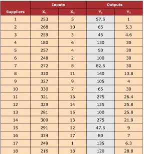
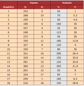
the original grey table is transformed to a table containing exact numbers. The data are presented in Tables 1, 2, 3, 4, 5 and 6 (In the source example, the values of the third column are grey).

Suppliers

Inputs Outputs

X1 X2 Y1 Y2

1 253 5 50 1

2 268 10 60 5.3

3 259 3 40 4.6

4 180 6 100 30

5 257 4 45 30

6 248 2 85 30

7 272 8 70 30

8 330 11 100 13.8

9 327 9 90 4

10 330 7 50 30

11 321 16 250 26.4

12 329 14 100 25.8

13 281 15 80 25.8

14 309 13 200 21.9

15 291 12 40 9

16 334 17 75 7

17 249 1 90 6.3

18 216 18 90 28.8

Suppliers

Inputs Outputs

X1 X2 Y1 Y2

1 253 5 53.75 1

2 268 10 62.5 5.3

3 259 3 42.5 4.6

4 180 6 115 30

5 257 4 47.5 30

6 248 2 92.5 30

7 272 8 76.25 30

8 330 11 120 13.8

9 327 9 97.5 4

10 330 7 57.5 30

11 321 16 262.5 26.4

12 329 14 112.5 25.8

13 281 15 90 25.8

14 309 13 237.5 21.9

15 291 12 43.75 9

16 334 17 77.5 7

17 249 1 112.5 6.3

18 216 18 105 28.8

Table 2. Original values for α=0.25

Suppliers

Inputs Outputs

X1 X2 Y1 Y2

1 253 5 57.5 1

2 268 10 65 5.3

3 259 3 45 4.6

4 180 6 130 30

5 257 4 50 30

6 248 2 100 30

7 272 8 82.5 30

8 330 11 140 13.8

9 327 9 105 4

10 330 7 65 30

11 321 16 275 26.4

12 329 14 125 25.8

13 281 15 100 25.8

14 309 13 275 21.9

15 291 12 47.5 9

16 334 17 80 7

17 249 1 135 6.3

18 216 18 120 28.8

Suppliers

Inputs Outputs

X1 X2 Y1 Y2

1 253 5 61.25 1

2 268 10 67.5 5.3

3 259 3 47.5 4.6

4 180 6 145 30

5 257 4 52.5 30

6 248 2 107.5 30

7 272 8 88.75 30

8 330 11 160 13.8

9 327 9 112.5 4

10 330 7 72.5 30

11 321 16 287.5 26.4

12 329 14 137.5 25.8

13 281 15 110 25.8

14 309 13 312.5 21.9

15 291 12 51.25 9

16 334 17 82.5 7

17 249 1 157.5 6.3

18 216 18 135 28.8

Table 4. Original values for α=0.75

Suppliers

Inputs Outputs

X1 X2 Y1 Y2

1 253 5 65 1

2 268 10 70 5.3

3 259 3 50 4.6

4 180 6 160 30

5 257 4 55 30

6 248 2 115 30

7 272 8 95 30

8 330 11 180 13.8

9 327 9 120 4

10 330 7 80 30

11 321 16 300 26.4

12 329 14 150 25.8

13 281 15 120 25.8

14 309 13 350 21.9

15 291 12 55 9

16 334 17 85 7

17 249 1 180 6.3

18 216 18 150 28.8

After measuring the efficiency for different levels

α

=

0, 0.25, 0.5, 0.75, 1

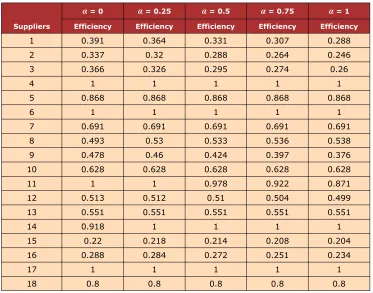
by DEA approach, the initial matrix of GRA method is the following:

Suppliers

α = 0 α = 0.25 α = 0.5 α = 0.75 α = 1 Efficiency Efficiency Efficiency Efficiency Efficiency

1 0.391 0.364 0.331 0.307 0.288

2 0.337 0.32 0.288 0.264 0.246

3 0.366 0.326 0.295 0.274 0.26

4 1 1 1 1 1

5 0.868 0.868 0.868 0.868 0.868

6 1 1 1 1 1

7 0.691 0.691 0.691 0.691 0.691

8 0.493 0.53 0.533 0.536 0.538

9 0.478 0.46 0.424 0.397 0.376

10 0.628 0.628 0.628 0.628 0.628

11 1 1 0.978 0.922 0.871

12 0.513 0.512 0.51 0.504 0.499

13 0.551 0.551 0.551 0.551 0.551

14 0.918 1 1 1 1

15 0.22 0.218 0.214 0.208 0.204

16 0.288 0.284 0.272 0.251 0.234

17 1 1 1 1 1

18 0.8 0.8 0.8 0.8 0.8

Table 6. Original matrix for different levels of α

In Table 6, the steps corresponding to the GRA method are discussed below.

4.1. Grey relation generation

Suppliers

α = 0 α = 0.25 α = 0.5 α = 0.75 α = 1 Efficiency Efficiency Efficiency Efficiency Efficiency

X0 1.000 1.000 1.000 1.000 1.000

1 0.219 0.187 0.149 0.125 0.106

2 0.150 0.130 0.094 0.071 0.053

3 0.187 0.138 0.103 0.083 0.070

4 1.000 1.000 1.000 1.000 1.000

5 0.831 0.831 0.832 0.833 0.834

6 1.000 1.000 1.000 1.000 1.000

7 0.604 0.605 0.607 0.610 0.612

8 0.350 0.399 0.406 0.414 0.420

9 0.331 0.309 0.267 0.239 0.216

10 0.523 0.524 0.527 0.530 0.533

11 1.000 1.000 0.972 0.902 0.838

12 0.376 0.376 0.377 0.374 0.371

13 0.424 0.426 0.429 0.433 0.436

14 0.895 1.000 1.000 1.000 1.000

15 0.000 0.000 0.000 0.000 0.000

16 0.087 0.084 0.074 0.054 0.038

17 1.000 1.000 1.000 1.000 1.000

18 0.744 0.744 0.746 0.747 0.749

Table 7. The normalized matrix

Where the reference sequence is defined as

X

0 =

(1, 1, 1, 1, 1)

.

4.2. The calculation of the grey relational coefficient

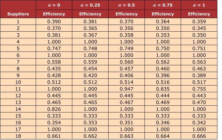
Using relation (13), the grey relational coefficients are calculated for all the values and the results are presented in Table 8.

Suppliers

α = 0 α = 0.25 α = 0.5 α = 0.75 α = 1 Efficiency Efficiency Efficiency Efficiency Efficiency

1 0.390 0.381 0.370 0.364 0.359

2 0.370 0.365 0.356 0.350 0.345

3 0.381 0.367 0.358 0.353 0.350

4 1.000 1.000 1.000 1.000 1.000

5 0.747 0.748 0.749 0.750 0.751

6 1.000 1.000 1.000 1.000 1.000

7 0.558 0.559 0.560 0.562 0.563

8 0.435 0.454 0.457 0.460 0.463

9 0.428 0.420 0.406 0.396 0.389

10 0.512 0.512 0.514 0.516 0.517

11 1.000 1.000 0.947 0.835 0.755

12 0.445 0.445 0.445 0.444 0.443

13 0.465 0.465 0.467 0.469 0.470

14 0.826 1.000 1.000 1.000 1.000

15 0.333 0.333 0.333 0.333 0.333

16 0.354 0.353 0.351 0.346 0.342

17 1.000 1.000 1.000 1.000 1.000

18 0.661 0.662 0.663 0.664 0.666

4.3. The calculation of the grey relational degree

The information in Table 6 is used to calculate the grey relational coefficients

γ

(

x

0j

,

xij

)

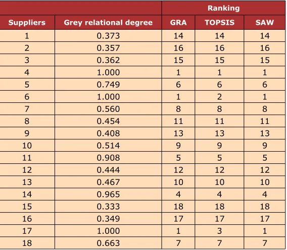
, grey

relational degree, ranking of suppliers based on GRA, ranking based on TOPSIS (Technique for Order-Preference by Similarity to Ideal Solution) and SAW (Sample Additive Weighting), and the results are presented in Table 9.

Ranking

Suppliers Grey relational degree GRA TOPSIS SAW

1 0.373 14 14 14

2 0.357 16 16 16

3 0.362 15 15 15

4 1.000 1 1 1

5 0.749 6 6 6

6 1.000 1 2 1

7 0.560 8 8 8

8 0.454 11 11 11

9 0.408 13 13 13

10 0.514 9 9 9

11 0.908 5 5 5

12 0.444 12 12 12

13 0.467 10 10 10

14 0.965 4 4 4

15 0.333 18 18 18

16 0.349 17 17 17

17 1.000 1 3 1

18 0.663 7 7 7

Table 9. The grey relational degree and ranking of suppliers

Suppliers Proposed Average MRA

1 [0.221,0.509] 14 14 14

2 [0.215,0.393] 16 16 16

3 [0.221,0.425] 15 15 15

4 [1.332,1.607] 3 3 3

5 [0.868,0.868] 4 7 7

6 [2.014,2.07] 2 2 2

7 [0.691,0.691] 8 8 8

8 [0.322,0.868] 12 11 9

9 [0.282,0.638] 13 13 13

10 [0.628,0.628] 9 9 10

11 [0.753,1.444] 6 5 5

12 [0.471,0.669] 11 12 12

13 [0.551,0.672] 10 10 11

14 [0.709,1.6] 7 4 4

15 [0.186,0.28] 18 18 18

16 [0.212,0.327] 17 17 17

17 [1.565,4.235] 1 1 1

18 [0.8,1.051] 5 6 6

Table 10. The efficiency of suppliers and the ranking results

4.4. Comparing the results of the model

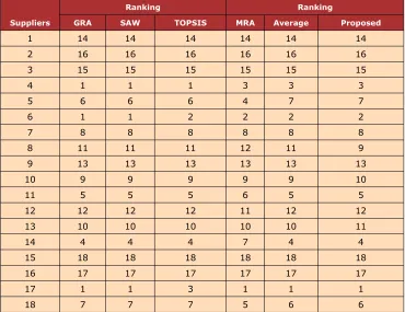
This section deals with ranking of suppliers. Table 11 presents the suppliers ranking done by all the aforementioned methods:

Suppliers

Ranking Ranking

GRA SAW TOPSIS MRA Average Proposed

1 14 14 14 14 14 14

2 16 16 16 16 16 16

3 15 15 15 15 15 15

4 1 1 1 3 3 3

5 6 6 6 4 7 7

6 1 1 2 2 2 2

7 8 8 8 8 8 8

8 11 11 11 12 11 9

9 13 13 13 13 13 13

10 9 9 9 9 9 10

11 5 5 5 6 5 5

12 12 12 12 11 12 12

13 10 10 10 10 10 11

14 4 4 4 7 4 4

15 18 18 18 18 18 18

16 17 17 17 17 17 17

17 1 1 3 1 1 1

18 7 7 7 5 6 6

According to Table 11, it is clear that GRA, TOPSIS, and SAW approaches have yielded the same results. In addition, by comparing the ranking obtained by GRA method with those of MRA, average, and the proposed approach, we notice that suppliers 17, 6, and 4 are selected as the efficient ones. It is worth reminding that the proposed approach works based on interval efficiency by solving the models introduced in (28) and (29).A Comparison demonstrates that the proposed approach provides satisfactory and acceptable results. Additionally, the amount of required computation associated with the proposed approach is less than that of model (27). Therefore, the proposed model in addition to providing acceptable results avoids time-consuming computation and consequently reduces the solving time. To name other advantage of the proposed model, we can point out that it is capable of making decision involving different levels of risk.

5. Conclusion and directions for future work

The critical role of suppliers in success of an organization makes the topic of evaluation and selection of suppliers a crucial task. Data envelopment analysis (DEA) has been widely applied in evaluating and selecting suppliers which considers the necessary inputs and outputs and then analyzes the efficiency of decision making units. Managers to make a decision can take two approaches: one is decision making in a static environment and the other is decision making in a stochastic environment. But the second one is closer to reality. In this regard, grey number theory is a tool to be used for coping with uncertainty. Hence, to make a decision in a stochastic environment, by applying a hybrid of data envelopment analysis and grey number theory, we can come to a right decisions. In this paper, a model for evaluating and selecting efficient suppliers under a stochastic environment is proposed in which a hybrid of data envelopment analysis and grey relational analysis is utilized. The proposed approach in addition to providing acceptable results avoids time-consuming computations and consequently reduces the solution time. To name another advantage of the proposed model, we can point out its capability of making decision involving different levels of risk. Finally, we present a novel ranking method for grey numbers.

References

Basnet, C., & Leung, J.M. Y. (2005). Inventory lot-sizing with supplier selection. Computers & Operations Research, 32(1), 1-14. http://dx.doi.org/10.1016/S0305-0548(03)00199-0

Charnes, A., Cooper, W.W., & Rhodes, E. L. (1978). Measuring the efficiency of decision making units. European Journal of Operational Research, 2(6), 429-44. http://dx.doi.org/10.1016/0377-2217(78)90138-8

Chen, W.H. (2005). Distribution system restoration using the hybrid fuzzy-grey method. IEEE Transactions on Power Systems, 20, 199-205. http://dx.doi.org/10.1109/TPWRS.2004.841234

Chen, Y., & Huang, P. (2007). Bi-negotiation integrated AHP in suppliers selection.

International Journal of Operations & Production Management, 27, 1254-1274.

http://dx.doi.org/10.1108/01443570710830629

Choy, K.L., & Lee, W.B. (2002). A generic tool for the selection and management of supplier relationships in an outsourced manufacturing environment: The application of case based reasoning. Logistics Information Management, 15, 235-253.

http://dx.doi.org/10.1108/09576050210436093

Cooper, W., Seiford, L.M., & Tone, K. (2000). Data Envelopment Analysis: A comprehensive text with models, applications, references and DEA-solver software. Kluwer Academic publisher, Boston.

Demirtas, E.A., & Üstün, Ö. (2008). An integrated multiobjective decision making process for supplier selection and order allocation. Omega, 36, 76-90.

http://dx.doi.org/10.1016/j.omega.2005.11.003

Deng, J. (1982). Control problems of grey systems. Systems and Control Letters, 1, 288-294.

http://dx.doi.org/10.1016/S0167-6911(82)80025-X

Farzipoor Saen, R. (2010). Developing a new data envelopment analysis methodology for supplier selection in the presence of both undesirable outputs and imprecise data.

International Journal of Advanced Manufacturing Technology, 51, 1243-1250.

http://dx.doi.org/10.1007/s00170-010-2694-3

Garfamy, R. (2006). A data envelopment analysis approach based on total cost of ownership for supplier selection. Journal of Enterprise Information Management, 19, 662-678.

http://dx.doi.org/10.1108/17410390610708526

Gencer, C., & Gürpinar, D. (2007). Analytic network process in supplier selection: A case study in an electronic firm. Applied mathematical modeling, 31, 2475-2486.

Ghodsypour, S.H., & O'Brien, C. (1998). A decision support system for supplier selection using an integrated analytic hierarchy process and linear programming. International Journal of Production Economics, 1, 56-57.

Hong, G., Park, S., Jang, D., & Rho, H. (2005). An effective supplier selection method for constructing a competitive supply-relationship. Expert Systems with Applications, 28, 629-639. http://dx.doi.org/10.1016/j.eswa.2004.12.020

Hou, J., & Su, D. (2007). EJB-MVC oriented supplier selection system for mass customization.

Journal of Manufacturing Technology Management, 18, 54-71.

http://dx.doi.org/10.1108/17410380710717643

Kahraman, C., Cebeci, U., & Ulukan, Z. (2003). Multi-criteria supplier selection using fuzzy AHP. Logistics Information Management, 16, 382-394. http://dx.doi.org/10.1108/09576050310503367

Lau, H., Lee, C., Ho. G., & Pun, K. (2006). A performance benchmarking system to support supplier selection. International Journal of Business Performance Management, 8, 132-151.

http://dx.doi.org/10.1504/IJBPM.2006.009033

Lin, C.T., Chang, C.W., & Chen, C.B. (2006). The worst ill-conditioned silicon wafer machine detected by using grey relational analysis. International Journal of Advanced Manufacturing Technology, 31, 388-395. http://dx.doi.org/10.1007/s00170-006-0685-1

Mendoza, A., Santiago, E., & Ravindran, A.R. (2008). A three-phase multicriteria method to the supplier selection problem. International Journalof Industrial Engineering, 15, 195-210.

Morán, J., Granada, E., Míguez, J.L., & Porteiro, J. (2006). Use of grey relational analysis to assess and optimize small biomass boilers. Fuel Processing Technology, 87, 123-127.

http://dx.doi.org/10.1016/j.fuproc.2005.08.008

Muralidharan, C., Anantharaman, N., & Deshmukh, S. (2002). A multi-criteria group decision making model for supplier rating. Journal of supply chain management, 38, 22-33.

http://dx.doi.org/10.1111/j.1745-493X.2002.tb00140.x

Narasimhan, R., Talluri, S., & Mendez, D. (2001). Supplier evaluation and rationalization via data envelopment analysis: an empirical examination. Journal of supply chain management, 37, 28-37. http://dx.doi.org/10.1111/j.1745-493X.2001.tb00103.x

Narasimhan, R., Talluri, S., & Mahapatra, S. (2006). Multiproduct, multicriteria model for supplier selection with product life-cycle considerations. Decision Sciences, 37, 577-603.

http://dx.doi.org/10.1111/j.1540-5414.2006.00139.x

Olson, D.L., & Wu, D. (2006). Simulation of fuzzy multiattribute models for grey relationships.

Saen, R. (2007). A new mathematical approach for suppliers selection: accounting for non-homogeneity is important. Applied mathematics and computation, 185, 84-95.

http://dx.doi.org/10.1016/j.amc.2006.07.071

Sarkar, A., & Mohapatra, P. (2006). Evaluation of supplier capability and performance: A method for supply base reduction. Journal of Purchasing and Supply Management, 12, 148-163. http://dx.doi.org/10.1016/j.pursup.2006.08.003

Talluri, S., & Baker, R. (2002). A multi-phase mathematical programming approach for effective supply chain design. European Journal of Operational Research, 141, 544-558.

http://dx.doi.org/10.1016/S0377-2217(01)00277-6

Talluri, S., & Narasimhan, R. (2005). A Note on a Methodology for Supply Base Optimization.

IEEE Transactions on Engineering Management, 52, 130-139.

http://dx.doi.org/10.1109/TEM.2004.839960

Talluri, S., Narasimhan, R., & Nair, A. (2006). Vendor performance with supply risk: a chance-constrained DEA approach. International Journal of Production Economics, 100, 212-222.

http://dx.doi.org/10.1016/j.ijpe.2004.11.012

Wu, H.H. (2002). A comparative study of using grey relational analysis in multiple attribute decision making problems. Quality Engineering, 15, 209-217. http://dx.doi.org/10.1081/QEN-120015853

Wu, T., Shunk, D., Blackhurst, J., & Appalla, R. (2007). AIDEA: a methodology for supplier evaluation and selection in a supplier-based manufacturing environment. International Journal of Manufacturing Technology and Management, 11, 174-192.

http://dx.doi.org/10.1504/IJMTM.2007.013190

Wu, D., & Olson, D.L. (2010). Fuzzy multiattribute grey related analysis using DEA. Computers and Mathematics with Applications, 60, 166-174. http://dx.doi.org/10.1016/j.camwa.2010.04.043

Journal of Industrial Engineering and Management, 2014 (www. jiem. org)

Article's contents are provided on a Attribution-Non Commercial 3. 0 Creative commons license. Readers are allowed to copy, distribute and communicate article's contents, provided the author's and Journal of Industrial Engineering and Management's names are included.