Humanoid Push Recovery

Humanoid Push Recovery

Benjamin Stephens

Email: [email protected]

Abstract—We extend simple models previously developed for humanoids to large push recovery. Using these simple models, we develop analytic decision surfaces that are functions of reference points, such as the center of mass and center of pressure, that predict whether or not a fall is inevitable. We explore three strategies for recovery: 1) using ankle torques, 2) moving internal joints, and 3) taking a step. These models can be used in robot controllers or in analysis of human balance and locomotion.

Index Terms—Dynamics, Robots, Robot dynamics

I. INTRODUCTION

We study humanoids as a way to understand humans. Any technology that is applied to aid humanoid motion can potentially be applied to help elderly or persons with disabilities walk with more stability and confidence. We want to understand what causes humanoids to fall, and what can be done to avoid it. Disturbances and modeling error are possible contributors to falling. For small disturbances, simply behaving like an inverted pendulum and applying a compen-sating torque at the ankle can be enough. As the disturbance increases, however, more of the body has to be used. Bending the hips or swinging the arms creates an additional restoring torque. Finally, if the disturbance is too large, the only way to stop from falling is to take a step.

In this paper, we unify simple models used previously by biomechanists and roboticists to explain humanoid balance and control. In Section I-A, we discuss previous work in detail and in Section I-B we summarize our models and balance strategies. Section II describes the simplest balance strategy for small disturbances, using only ankle torques to stabilize. Section III employs an expanded model to allow use of the rest of the body. Finally, in Section IV, we discuss the choice of step location when balance strategies fail.

The main contributions of this paper are the unification of models and strategies used for humanoid balance and the development of decision surfaces that define when each strategy is necessary and successful at preventing a fall. These decision surfaces are defined as functions of reference points, such as the center of mass and center of pressure, that can be measured or calculated easily for both robots and humans. We assume that both ankle and internal joint actuation are available and used in balance recovery.

A. Related Work

The problem of postural stability in humanoids has been a subject for many years. Vukobratovic, et.al. was the first to

Fig. 1. The three basic balancing strategies. The green dot represents the center of mass, the magenta dot represents the center of pressure, and the blue arrow represents the ground reaction force. 1. CoP Balancing (“Ankle Strategy”) 2. CMP Balancing (“Hip Strategy”) 3. Step-out

apply the concept of the ZMP, or zero moment point, to biped balance [1]. Feedback linearizing control of a simple double-inverted pendulum model using ankle and hip torques was used by Hemami,et.al.[2]. Stepping to avoid fall was also studied by Goddard, et.al. [3], using feedback control of computed constraint forces derived from Lagrangian dynamics.

Modern bipedal locomotion research has been heavily in-fluenced by Kajita, et.al. and their Linear Inverted Pendu-lum Model (LIPM) [4]. It is linearized about vertical and constrained to a horizontal plane, so it is a one-dimensional linear dynamic system representing humanoid motion. When considering ankle torques and the constraints on the location of the ZMP, or zero moment point, it has also been referred to as the “cart-on-a-table” model. An extension to the LIPM is the AMPM, or Angular Momentum inducing inverted Pendulum Model [5], which generates momentum by applying a non-centroidal torque to the center of mass (CoM).

used for large disturbances takes a step in order to increase or move the feasible area for the CoP (and equivalently the CMP). In stepping, he says that the swing leg impact absorbs kinetic energy and the step distance determines the magnitude of energy absorbed.

Goswami,et. al.[7] also considered the strategy of inducing non-zero moment about the CoM in order to balance in detail. They define theZRAM point(Zero Rate of change of Angular Momentum), which is identical to the CMP. In fact, there have been numerous attempts to identify important “points” in humanoid balancing and locomotion [8].

Pratt, et. al. [9] attempted to formulate the control and stability of biped walking using more meaningful velocity formulations. They argued that traditional approaches, like Poincare Maps and ZMP trajectories, are not suitable for fast, dynamic motions. They suggest that angular momenta about the center of pressure and the center of mass are important quantities to regulate. Their velocity-based formulations and “Linear Inverted Pendulum Plus Flywheel Model” [10] were used to formulate the “capture region,” where the robot must step in order to catch itself from a fall. Sometimes the capture region is outside the range of motion and the robot takes more than one step in order to recover. The model they use is simple and allows regulation of angular momentum, but in their formulation they do not consider impact energy losses or the effect of ankle torques.

The research performed by roboticists has been paralleled by the work of biomechanists and physical therapists. These researchers similarly use inverted pendulum models to explain balance and walking [11]. The “hip strategy” and “ankle strategy,” described by Horak and Nashner [12], have long been dominant descriptions of balance control in humans. Makai et. al. studied the interaction of these “fixed-base” strategies with “change-of-support” strategies in human test subjects [13]. They argue that these strategies occur in parallel, rather than sequentially, and that humans will take a step much before they reach the stability boundary for standing in place. An explanation for their findings is they only consider the position of the CoM as the defining measure of stability. It was soon observed that the use of CoM velocity in addition to position was a better measure of stability [14] [15].

B. Balance Models and Strategies

Here we explore different models and strategies used for humanoid balance. There are three basic strategies:

1) CoP Balancing (ankle strategy) 2) CMP Balancing (hip strategy) 3) Stepping (change-of-support strategy)

Generally, these strategies can be employed sequentially from top to bottom, advancing to the next if the current strategy is inadequate. As shown in Fig. 1, the effective horizontal force on the center of mass, equal to the horizontal ground reaction force, can be increased (CMP Balancing) or moved (Stepping) if simple CoP Balancing is not enough.

Our primary goal is to determine decision surfaces that describe when a particular strategy should be used. Real

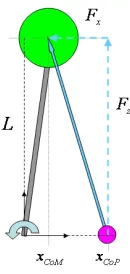
Fig. 2. When only applying ankle torque, the ground reaction force points from the center of pressure (CoP) to the center of mass (CoM), creating zero moment about the CoM.

humanoid robots will have many more degrees of freedom and complicated control problems, but by describing their motion in terms of these dimensionally-reduced quantities, such as center of mass and center of pressure, we create useful approximations. Reduced dimensionality also makes it easier to visualize motions, aiding in intuition and understanding.

II. COP BALANCING

In this section we explore the simplest balancing strategy which uses ankle torque to apply a restoring force, while other joints are fixed. This is often referred to as the “ankle strategy.” The location of the CoP is proportional to ankle torque, and therefore the limits on the position of the CoP correspond to torque limits at the ankle.

The stability of the robot can be determined by the state-space location,(xCoM,x˙CoM), of the center of mass. We want

to find the limits on the state of the center of mass that can be stopped from leaving the base of support by a saturated ankle torque. The relation between horizontal acceleration of the CoM and the tangential ground reaction force,Fx, is

¨

xCoM= Fx

m (1)

whereFxis the tangential ground reaction force. If only ankle

torque is used, then the ground reaction force points from the CoP to the CoM, as shown in Fig. 2. Then Fx is related to

the normal force, Fz, by

Fx=

Fz

zCoM(xCoM−xCoP) (2)

wherexCoMandxCoPare the locations of the CoM and CoP,

respectively. If we assume the vertical motion of the CoM is negligible, then Fz = mg. Also, if we assume the ankle

torque is saturated with the CoP at the edge of the foot at

xCoP=δ±, whereδ− andδ+ are the back and front edges of

support region, respectively, then the maximum acceleration is given by

¨

xmax_CoM= g

L(xCoM−δ

±_{), (3)}

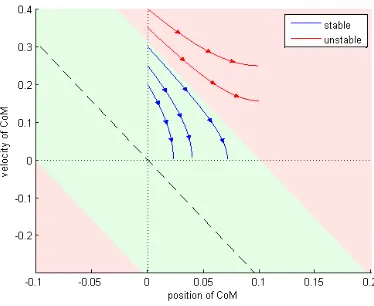
(a) These are open loop trajectories starting from standing straight up and experiencing an impulse push and using a saturated ankle torque only. All trajectories that start in the green region are stable and all that start in the red will fall.

(b) These are feedback trajectories created by a PD controller (with torque limits) on the ankle joint of a single inverted pendulum. The stability region derived from the linear inverted pendulum model closely predicts the stability of the nonlinear inverted pendulum.

Fig. 3. Trajectories generated by open-loop and closed-loop CoP balancing.

into the constraint,δ−< xCoM(t)< δ+, we get

δ− <x˙CoM

ω +xCoM< δ +

(4)

whereω2_{=g/L. This constraint represents a decision surface}

in CoM state space, as shown in Fig. 3(a), that can be constantly monitored. If the state of the humanoid is outside of this decision surface, then ankle torque alone cannot restore balance and either a different balance strategy is needed or a step should be initiated to prevent falling. These decision surfaces are evaluated on a single inverted pendulum using a PD ankle controller with saturation, in Fig. 3(b).

III. CMP BALANCING

The CMP, or centroidal moment point, is equal to the CoP in the case of zero moment about the center of mass. For the ankle strategy, this is always the case. However, humanoids have many internal joints, particularly the torso and arms, that allow them to apply a torque about the CoM. For a non-zero

Fig. 4. Internal joint torques create a torque about the CoM. This is reflected by the ground reaction force, which emmits from the CoP but does not necessarily point through the CoM. The equivalent force that points through the CoM begins from the CMP.

centroidal moment, the CMP moves beyond the edge of the foot.

We model the internal joint torques by treating the CoM, or body, as a flywheel that can be torqued directly, as shown in Fig. 4. This model is an extension of the model used by Pratt et. al. [10] to allow for an ankle torque. Compared to Eq.(3), which is the maximum acceleration using only ankle torque, the maximum acceleration using both ankle torque and a flywheel torque is

¨

xmaxCoM= g

L(xCoM−δ

±_±τmax

mg ), (5)

The additional torque term, due to the momentum generating flywheel, allows for a greater maximum horizontal force. However, the flywheel really represents inertia of the torso and upper body and should be subject to joint limit constraints. The linear dynamics of the system can be written as

¨

x−ω2x = −ω2

δ+ τ

mg

(6)

Iθ¨ = τ (7)

Initially, a large, torque can be used to accelerate the CoM backwards. Soon after, however, a reverse torque must be applied to keep the flywheel from exceeding joint limits. The goal of the flywheel controller is to return the system to a region that satisfies Eq.(4) that avoids exceeding the joint limit constraints. If this cannot be achieved, then a step will be required.

Like CoP balancing, we determine the decision surfaces by considering the largest control action possible. For CMP balancing, this is accomplished using a saturated ankle torque and bang-bang control of the flywheel. Afterwards, we develop a practical controller using optimal control that demonstrates the effect of these decision surfaces.

A. Bang-Bang Control

A bang-bang control input profile to the flywheel can be used to generate analytic solutions. The bang-bang function,

(a) The phase plot shows how the system responds to bang-bang control of the flywheel. All trajectories, except the one that starts outside of the stable regions, can be stabilized by bang-bang control.

(b) These time plots show the flywheel response to bang-bang control. In this case,θmax= 1.0rad,I= 10kgm2 andτmax=

100N m. The vertical dashed line representsTmax, the maximum

time for which the flywheel can be spun up.

Fig. 5. Bang-Bang trajectories and system outputs. Only the phase state of the CoM is shown in the top figure, whereas the flywheel state is shown in the bottom figure.

maximum negative torque for a period of T2 and is zero afterwards. This function can be written as

τbb(t) =τmax+ 2τmaxu(t−T1)−τmaxu(t−T2), (8)

whereu(t−T∗)is a step function at time,t=T∗. The goal is to return the system to a state that satisfies Eq.(4) att=T2,

δ− <x˙(T2)

ω +x(T2)< δ

+ ₍₉₎

If the system is returned to this state, CoP balancing can be used to drive the system back to a stable state and the the flywheel can be moved back to zero. We combine Eqs. (5) & (9) to solve for bounds. We assume the flywheel starts with

θ(0) = 0andθ˙(0) = 0. First, by integrating Eq.(7) using the bang-bang input,τbb(t), and imposing the constraint,θ˙(T2) =

0, we get

˙

θ(T2) = τmax

I (T2−2(T2−T1)) = 0, (10)

(a) The phase plot shows how the system can be driven back into the stable region using optimal control. Notice that the unstable starting states are correctly predicted.

(b) Receding horizon control, with a look-ahead time of1.0s, was used to drive the system back to the origin after an initial impulse disturbance gives a non-zero velocity of the CoM. Notice that for the small perturbation, the optimal controller does not use the flywheel much.

Fig. 6. CMP balancing using optimal control. The region predicted by the bang-bang controller correctly predicts whether or not the system can be stabilized.

which requires thatT2= 2T1= 2T. Additionally, integrating once more, and using the joint limit constraint,θ(2T)< θmax,

we find that

θ(2T) = τmax

I T 2_{< θ}

max (11)

which meansT has a maximum value,

Tmax=

r

Iθmax

τmax (12)

We can again use the derivations from Appendix A to solve the differential equation in Eq.(6). We find that

x(2T) = δ+ (x0−δ) cosh(2ωT) +x˙0

ω sinh(2ωT)

+ τmax

mLω2(−cosh(2ωT) + cosh(ωT)−1)

˙

x(2T) = ω(x0−δ) sinh(2ωT) + ˙x0cosh(2ωT)

+τmax

See [10] for more detailed derivations. Now, inserting this into the right-side inequality in Eq.(9) and using the identity, sinh(x) + cosh(x) =ex_{, we get}

x0−δ++

˙ x0 ω − τmax mg

e2ωT +2τmax

mg e

ωT

−τmax

mg <0 (13)

x0−δ−+x0˙

ω + τmax

mg

e2ωT −2τmax

mg e

ωT ₊τmax

mg >0 (14)

If we assume the worst-case, T =Tmax, then the inequalities from above become

δ−−τmax

mg (e

ωTmax₋₁₎2_{< x0+}x˙0

ω < δ +

+τmax

mg (e

ωTmax₋₁₎2

(15) If the system is within these decision surfaces, then the system can be stabilized using CMP balancing control. If the system is outside, however, it will have to take a step to avoid falling over. Of course, these bounds overlap the bounds in Eq.(4), so the decision of whether or not to use CMP balancing for small perturbations is a decision to be made. However, keeping the torso and head upright is usually a priority, so CoP balancing should be used whenever possible.

B. Optimal Control

We can alternatively solve this problem using optimal con-trol. Using this method, we can test whether or not the bounds defined using the bang-bang controller above are realistic. The equations of motion from Eqs. (6) & (7) can be transformed into the first-order system,

    ˙ x ˙ θ ¨ x ¨ θ     =    

0 0 1 0

0 0 0 1

ω2 0 0 0

0 0 0 0

        x θ ˙ x ˙ θ     +     0 0 0 0

−ω2 _−(mL)−1

0 I−1

    δ τ (16)

We can discretize these equations, into Xi+1 =AXi+BUi,

and generate optimal controls. The quadratic cost function used is

J =

N

X

i

γ(N−i)

X_iTQXi+UiTRUi (17)

whereXi is the state,Ui= (δi, τi)T is the action, and γ <1

is a discount factor. The discount factor increases the cost with

i. Fig. 6 shows simulations of the optimal control, where the manually adjusted parameters we used were

Q= diag[103,103,10,10]

R= diag[10−2_,10−5_] γ= 0.9

Receding horizon control, with a look-ahead time of 1.0s

and a timestep of 0.02s, makes N = 50. At each timestep, a quadratic programming problem is solved to generate the optimal control trajectory over the 1.0s horizon. Notice that

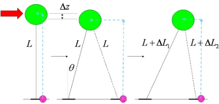
Fig. 7. The model used for step-out has a point mass at the hip with massless, extendable legs. After impact, the body moves horizontally only.

Fig. 8. The impact model used assumes that the vertical velocity of the CoM instantaneously goes to zero during the impact. The impulsive force that results in this change also results in a decrease in horizontal velocity.

one of the trajectories starts inside the CoP Balancing region and the optimal controller does not use the flywheel while another starts outside of the stable regions and the controller cannot stabilize it, as expected.

IV. STEPPING

For even larger disturbances, no amount of body torquing will result in balance recovery. In this case, it is necessary to take a step. Taking a step moves the support region to either the area between the rear leg heel and the forward leg toe (double support) or the area under the new stance foot (single support). Since a larger disturbance requires a larger restoring force, this generally leads to larger steps. However, the location of the best foot placement is also affected by kinematic constraints and impact dynamics.

Fig. 9. Starting from an unstable state, taking a step causes a discontinuous jump into a stable region. The transitions shown are the ones that satisfy Eq.(21). In this figure, velocities are scaled by√zso each system behaves likeL= 1.

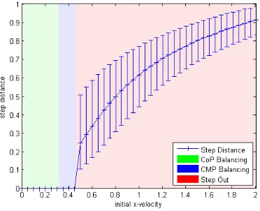
Fig. 10. The optimal step distance vs. the initial horizontal velocty of the CoM. The shaded regions show where the various recovery strategies should be employed. The error bars show the bounds on step distance that results in a stable state after impact. The optimal step distance is not half way between the bars because of the nonlinear relationship.

Considering the point mass,m, at the end of the pendulum of length, L, then the horizontal and vertical velocities are given by

vx

vz

=−L

cosθ

sinθ

˙

θ (18)

During the impact, an impulsive force causes a discontinous change in these velocities, as illustrated in Fig. 8, given by the relationship,

4vx

4vz

= v

+

x −vx−

vz+−vz−

= tanθ (19)

We assume that the vertical velocity goes to zero, orv+

z = 0,

so 4vz=−v−z. So the change in horizontal velocity is given

by

4vx=−v−z tanθ=Lθ˙sinθtanθ (20)

A. Choosing Step Length

The best choice for step length is the step that results in a transition into a state that the most robust. Upon impact, there is a discontinuous jump in the CoM phase plane. The new position of the CoM is behind the stance foot and the velocity is the same, so the jump is horizontal, as illustrated by the dotted lines in Fig. 9. After the impact, we want the system to be stabilizable using CoP or CMP Balancing. The best step is one that lies in the middle of the stable region. We want to find the step that results in the relationship,

vx++x

r

g

z = 0 (21)

which places the system on the black dashed line in Fig. 9. A system starting on this line will be open-loop stable using zero ankle torque. Because there is a large margin for errors and disturbances, this is the most robust foot placement.

We can use Eqs. (18),(20)&(21) to derive a relationship for the step distance. The relationship, in terms of the angle θ, just before impact, is

˙

θ=ωsinθcos 1/2_θ

cos 2θ (22)

This is the equation of the blue dash-dotted line in Fig. 9 that intersects the trajectories of the pendulum at the optimal step distance. There is no analytic solution for the trajectory of the pendulum, but numerical integration is used to find this intersection. Fig. 10 shows the optimal step distance for starting at a range of initial horizontal CoM velocities. For illustration, error bars are attached to each point showing the range of step distances that would also result in a stable state.

V. SUMMARY ANDFUTUREWORK

We have shown how to use simple models to approximate the motion of humanoids in the case of recovering from large disturbances. These simple models are built upon the prior work of biomechanics and robotics researchers. From these models, we produced realistic bounds that can be applied to complex humanoid robots or human subjects to predict a fall or choose a balance strategy.

In the near future, these balance strategies will be applied to a hydraulic humanoid robot made by Sarcos. Unlike many previous balancing controllers for humanoid robots, we plan to have our robot recover from very large disturbance forces. We will use the upper body, including torso and arms to aid balance, similar to the flywheel model in Section III.

APPENDIXA

This appendix gives the detailed derivation of the solution of the differential equation in Eq.(3). For simplicity, the equation can be written as

¨

x−ω2x=f (23)

where ω2 _{=g/L andf =−gδ/L. The initial conditions are} x(0) =x0andx˙(0) = ˙x0. The equation has a solution of

x(t) = _f

ω2 +x0

cosh(ωt) +x0˙

ω sinh(ωt)− f

ω2 (24)

ACKNOWLEDGMENTS

This material is based upon work supported in part by the National Science Foundation under grants CNS-0224419, DGE-0333420, ECS-0325383, and EEC-0540865.

REFERENCES

[1] M. Vukobratovic, A. A. Frank, and D. Juricic, “On the stability of biped locomotion,”IEEE Transactions on Biomedical Engineering, pp. 25–36, January 1970.

[2] H. Hemami and P. Camana, “Nonlinear feedback in simple locomotion systems,”IEEE Transactions on Automatic Control, vol. 21, no. 6, pp. 855–860, December 1976.

[3] R. Goddard, H. Hemami, and F. Weimer, “Biped side step in the frontal plane,” IEEE Transactions on Automatic Control, vol. 28, no. 2, pp. 179–187, February 1983.

[4] S. Kajita and K. Tani, “Study of dynamic biped locomotion on rugged terrain-derivation andapplication of the linear inverted pendulum mode,” inProceedings of the IEEE International Conference on Robotics and Automation, vol. 2, April 1991, pp. 1405–1411.

[5] S. Kudoh and T. Komura, “c2 continuous gait-pattern generation for biped robots,” inProceedings of the IEEE/RSJ International Conference on Intelligent Robots and Systems, vol. 2, October 2003, pp. 1135– 1140. [6] A. Hofmann, “Robust execution of bipedal walking tasks from biome-chanical principles,” Ph.D. dissertation, Massachusetts Institute of Tech-nology, January 2006.

[7] A. Goswami and V. Kallem, “Rate of change of angular momentum and balance maintenance of biped robots,” inProceedings of the 2004 IEEE International Conference on Robotics and Automation, vol. 4, 2004, pp. 3785– 3790.

[8] M. B. Popovic, A. Goswami, and H. Herr, “Ground reference points in legged locomotion: Definitions, biological trajectories and control implications,”The International Journal of Robotics Research, vol. 24, no. 12, pp. 1013–1032, 2005.

[9] J. Pratt and R. Tedrake, “Velocity based stability margins for fast bipedal walking,” in First Ruperto Carola Symposium in the International Science Forum of the University of Heidelberg entitled “Fast Motions in Biomechanics and Robots”, Heidelberg Germany, September 7-9 2005. [10] J. Pratt, J. Carff, S. Drakunov, and A. Goswami, “Capture point: A step toward humanoid push recovery,” in 6th IEEE-RAS International Conference on Humanoid Robots, December 2006, pp. 200–207. [11] D. Winter, “Human balance and posture control during standing and

walking,”Gait and Posture, vol. 3, no. 4, pp. 193–214, December 1995. [12] F. Horak and L. Nashner, “Central programming of postural movements: adaptation to altered support-surface configurations.”Journal of Neuro-physiology, vol. 55, no. 6, pp. 1369–1381, 1986.

[13] B. Makai and W. McIlroy, “The role of limb movements in maintaining upright stance: the ”change-in-support” strategy,” Physical Therapy, vol. 77, no. 5, pp. 488–507, May 1997.

[14] Y. Pai and J. Patton, “Center of mass velocity-position predictions for balance control,”Journal of Biomechanics, vol. 30, no. 4, pp. 347–354, 1997.