Open Access
Research article
On the ease of predicting the thermodynamic properties of
beta-cyclodextrin inclusion complexes
Andreas Steffen
1and Joannis Apostolakis*
2Address: 1Max-Planck-Institut für Informatik, Computational Biology and Applied Algorithmics, Stuhlsatzenhausweg 85, 66123 Saarbrücken,
Germany and 2Ludwig-Maximilians-Universität München, Institut für Informatik, Lehr- und Forschungseinheit für Bioinformatik, Amalienstrasse
17, 80333 München, Germany
Email: Andreas Steffen - [email protected]; Joannis Apostolakis* - [email protected] * Corresponding author
Abstract
Background: In this study we investigated the predictability of three thermodynamic quantities related to complex formation. As a model system we chose the host-guest complexes of β -cyclodextrin (β-CD) with different guest molecules. A training dataset comprised of 176 β-CD guest molecules with experimentally determined thermodynamic quantities was taken from the literature. We compared the performance of three different statistical regression methods – principal component regression (PCR), partial least squares regression (PLSR), and support vector machine regression combined with forward feature selection (SVMR/FSS) – with respect to their ability to generate predictive quantitative structure property relationship (QSPR) models for ∆G°, ∆H° and ∆S° on the basis of computed molecular descriptors.
Results: We found that SVMR/FFS marginally outperforms PLSR and PCR in the prediction of ∆G°, with PLSR performing slightly better than PCR. PLSR and PCR proved to be more stable in a nested cross-validation protocol. Whereas ∆G° can be predicted in good agreement with experimental values, none of the methods led to comparably good predictive models for ∆H°. In using the methods outlined in this study, we found that ∆S° appears almost unpredictable. In order to understand the differences in the ease of predicting the quantities, we performed a detailed analysis. As a result we can show that free energies are less sensitive (than enthalpy or entropy) to the small structural variations of guest molecules. This property, as well as the lower sensitivity of ∆G° to experimental conditions, are possible explanations for its greater predictability.
Conclusion: This study shows that the ease of predicting ∆G° cannot be explained by the predictability of either ∆H° or ∆S°. Our analysis suggests that the poor predictability of T∆S° and, to a lesser extent, ∆H° has to do with a stronger dependence of these quantities on the structural details of the complex and only to a lesser extent on experimental error.
Background
Cyclodextrins (CDs) are cyclic oligomers of α-D-Glucose, which can be categorised into four types: α-, β-, γ- and δ -CDs, corresponding to 6, 7, 8 or 9 α-D-glucose units. The
shape of CDs has been described as torus- or doughnut-like, reflecting the existence of a cavity within the mole-cule. The exterior region of the CD, which is populated with hydroxyl groups, is hydrophilic, whereas the cavity is
Published: 15 November 2007
Chemistry Central Journal 2007, 1:29 doi:10.1186/1752-153X-1-29
Received: 18 September 2007 Accepted: 15 November 2007
This article is available from: http://journal.chemistrycentral.com/content/1/1/29
© 2007 Steffen et al
dominated by hydrophobic interactions, enabling CDs to form relatively strong complexes with hydrophobic guests. The hydrophobicity of the CDs' exterior ensures their water solubility, a property that results in their being potential solubilisers [1].
The size of the molecules that can be bound by a particu-lar CD is related to the size of the cavity. α-CDs bind alkyl-chains of various lengths, whilst benzene, for instance, is seen to be too large. β-CDs cavities can complex more bulky molecules, such as adamantane, naphthalene or various benzene derivatives. γ-CDs can bind annelated ring systems and even buckyballs up to C60. The ability of CDs to bind molecules of particular sizes has been termed 'size recognition' [1,2].
β-CDs in particular have proven to be in high demand in the pharmaceutical industry because their cavities seem to be almost 'predestined' to bind drug-size molecules. Sev-eral formulations are on the marketplace in which β-CDs are applied as solubilisers of insoluble drugs [3-7]. Other industrial applications have been reported in the food industry, where CDs have been used to protect flavours or vitamins from oxidation [8]. It is therefore felt that an ability to predict the thermodynamic properties of this particular host-guest system could potentially have a direct impact on the development of novel pharmaceuti-cal formulations.
Some time has been spent on studying and predicting the binding free energies (∆G°) of CD inclusion complexes using computational methods [9,10]. Amongst these sta-tistical methods, those based on multiple regression [11,12] or neural nets [13] have particularly proven to lead to robust prediction models.
In this study we investigate the predictability of the ther-modynamic quantities relevant to complex formation, i.e. the free energy change ∆G°, the change of enthalpy ∆H°
and the change of entropy ∆S°. The study is combined with a detailed performance comparison of three different types of statistical regression methods, namely principal components regression (PCR) [14], partial least squares regression (PLSR) [14] and support vector regression with forward feature selection (SVMR/FFS) [15,16]. Whereas the first two methods are well established in the field of cheminformatics, the latter is a relatively new machine learning technique, which has been successfully applied in recent research projects [17,18]. We have also reported its application as a valuable tool for increasing hit rates in similarity based virtual screenings [19].
Our study shows that the ease of predicting ∆G° cannot be explained by the predictability of either ∆H° or ∆S°. We
shall discuss this finding in the context of a concise anal-ysis of the experimental accuracy of thermodynamic data.
Results and discussion
In this study we investigated the predictability of the experimental thermodynamic data for 176 guest mole-cules of β-CD (see additional file 1: Table 1). For all mol-ecules we had experimental values for the three fundamental thermodynamic quantities, entropy change (T∆S°), enthalpy change (∆H°) and the Gibbs free energy of binding (∆G°). Statistical models were developed to predict each of these properties on the basis of computed molecular descriptors. We applied three different types of regression methods: principal component regression (PCR), partial least squares regression (PLSR) and support vector machine regression with forward feature selection (SVMR/FFS). To validate and assess our models we per-formed tenfold cross-validation and nested cross-valida-tion protocols.
Comparison of the regression methods
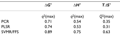
The results of the cross-validations are outlined in Table 1. We can express the cross-validation parameter q2, which
includes the prediction errors, as:
where σ2(...) = variance of the respective quantity in
brack-ets, ∆y is the deviation between prediction and experimen-tal value, and y is the quantity being predicted.
On applying PCR to predict ∆G°, ∆H° and T∆S°, the high-est cross-validation q2 values obtained are 0.71, 0.54 and
0.35 respectively (Table 1). PLSR leads to models with maximal q2 values for the three properties of 0.74, 0.53
and 0.31, respectively. The highest q2 values obtained are
for SVMR/FFS, namely, 0.89, 0.75 and 0.63 respectively.
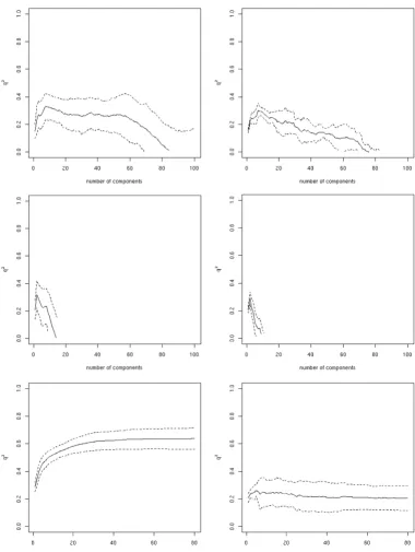
The shape of the curve when plotting the number of com-ponents or descriptors against q2 is characteristic for each
of the regression methods (Figure 1 – the left column shows a representative example). PLSR directly steers
q y y 2 1 2 2 = −σ
σ ( )
( ) , ∆
Table 1: Comparison of the regression methods for ten-fold cross validation. The maximal q2 values are reported for each
thermodynamic parameter.
∆G° ∆H° T∆S°
q2(max) q2(max) Q2(max)
PCR 0.71 0.54 0.35
PLSR 0.74 0.53 0.31
towards the maximal q2 value and thus reaches its peak
with only a few components. After this maximum, the q2
value decreases slightly, levels off, until dropping drasti-cally at one point. The curves for PCR look somewhat dif-ferent; the maximum q2 is reached with significantly more
components, and in-between local minima are also seen to exist. The differences in the shape of the curves can be explained by the way in which the components are obtained. While in PLSR the components are derived from the cross-covariance between the descriptors and the pre-dictors, in PCR the components are only derived from the descriptor matrix. For SVMR/FFS the q2 value increases
continuously with each added descriptor until it plateaus at the maximal q2 value. This continuous increase in the q2
value is due to the FFS selection criterion, which includes the descriptor that shows the highest improvement in cross-validation performance.
In order to validate accurately the statistical models we performed the nested cross-validation protocol as described by Ruschhaupt et al. [20]. This type of valida-tion gives an accurate estimate of the reliability of predict-ing external data. The method consists of inner and outer cross-validation loops. In the inner loop 10-fold cross-val-idation is used to identify the optimal settings for the complete algorithm that are then used for the outer loop. In the outer loop the performance of the best model obtained from the inner loop is tested on unseen data. Thus the test-sets in the outer loop do not in any way influence the training, with the performance of the learner on these test sets being an objective measure of its expected performance on similar data. Compared to the typical validation by external test-sets, this approach has an advantage of being less dependent on the partitioning into test and training sets, as each data point is part of the test-set exactly once. For each regression method this pro-cedure was performed three times resulting in nine differ-ent models and prediction assessmdiffer-ents. A more detailed description of nested cross validation is outlined in the methods section.
The PCR model predicts the molecules' ∆G° values in the outer loop with a q2 of 0.69 ± 0.03 to the experimentally
determined values, while PLSR gives a q2 of 0.69 ± 0.03
and SVMR/FFS a value of 0.71 ± 0.03 (Figure 1 and Table 2). In the case of SVMR/FFS, a drastic decrease in the outer loop's q2, in comparison to that of the inner loop, can be
observed. The maximal obtained q2 value in the inner
loop is 0.87, whereas in the outer loop a value of only 0.74 was found. PLSR and PCR show more stable behav-iour with comparable q2 values for the inner and the outer
loops. The correlations obtained for the prediction of ∆H°
and T∆S° (see Figure 2 and Table 3, and Figure 3 and Table 4 respectively) are clearly below those obtained for the prediction of ∆G° with all regression methods. For
both ∆H° and T∆S° none of the regression methods resulted in a q2 value of above 0.5 in the outer loop. This
finding in particular highlights the risk of over-fitting the SVMR/FFS model to the data, because in the ten-fold cross-validation comparably good correlations were obtained even for ∆H° and T∆S°. The over-fitting of the SVMR/FFS model has mainly to do with the forward fea-ture selection algorithm, which uses the squared correla-tion coefficient to choose the next descriptor in the iteration. Thus the execution of a nested cross validation is essential for obtaining a realistic estimate of the method's predictive ability.
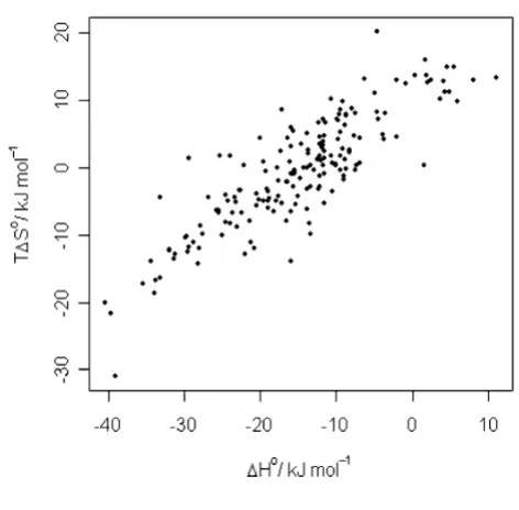
Predictability of different thermodynamic quantities The relationship between the three quantities is given, on the one hand, by classical thermodynamics (∆G° = ∆H°
-T∆S°), and the empirical finding of enthalpy-entropy compensation, on the other [21]. In Figure 4 we can observe the enthalpy-entropy compensation effect for the current data set. Surprisingly, for all regression methods the best predictions obtained were those for ∆G°. For
T∆S°, in particular, no predictive regression models could be generated with any of the methods. One possible rea-son for the differing predictabilities of the three quantities has been suggested by Sharp [21]. In an analysis of the thermodynamics of three different protein systems, Sharp suggests that the most probable explanation for entropy-enthalpy compensation is the higher experimental error involved in the determination of ∆H° and T∆S° [21]. If ∆G° can be measured reliably, while there is significant error in the determination of ∆H° and T∆S°, the last two quantities will vary significantly and in a correlated man-ner, because of the relationship ∆G° = ∆H°-T∆S°. This explanation agrees with the apparent difficulties that we face in predicting ∆H° and T∆S° in comparison to ∆G°. Furthermore, it has been observed that experimental parameters have a significantly higher influence on ∆H°
and T∆S° than on ∆G°. Ross et al., for example, measured the thermodynamic properties of the complex formed from cyclohexanol and β-CD at four different tempera-tures (288 – 318 K) [22]. While the ∆G° values were about the same in all measurements (16.3 ± 0.2 kJmol-1), those
for ∆H° varied between -2.8 and -13.0 kJmol-1 and T∆S°
13.2 and 3.6 kJmol-1. The stronger dependence of ∆H°
and T∆S° on experimental parameters leads to larger errors, particularly when data from different laboratories are used. This was apparent in our study, and for this rea-son, the explanation for the existence of different experi-mental accuracies appears plausible.
addi-Dependence of the cross-validation coefficient q2 (∆G°) on the number of components/descriptors integrated into a model for the inner (left column) and the outer loop (right column) of the nested-cross validation for all three methods (top to bottom: PCR, PLS, and SVM)
Figure 1
Dependence of the cross-validation coefficient q2 (∆G°) on the number of components/descriptors integrated into a model for
Dependence of the cross-validation coefficient q2 (∆H°) on the number of components/descriptors integrated into a model for the inner (left column) and the outer loop (right column) of the nested-cross validation for all three methods (top to bottom: PCR, PLS, and SVM)
Figure 2
Dependence of the cross-validation coefficient q2 (∆H°) on the number of components/descriptors integrated into a model for
Dependence of the cross-validation coefficient q2 (T∆S°) on the number of components/descriptors integrated into a model for the inner (left column) and the outer loop (right column) of the nested-cross validation for all three methods (top to bottom: PCR, PLS, and SVM)
Figure 3
Dependence of the cross-validation coefficient q2 (T∆S°) on the number of components/descriptors integrated into a model for
tional data if multiple measurements for a guest molecule were listed in Rekharsky's review [23]. For those com-pounds for which we had independent data from other published studies, we calculated the standard deviations for ∆G°, ∆H° and T∆S°, and averaged these over all com-pounds; the respective values obtained being 1.8 kJmol-1,
2.1 kJmol-1, and 2.7 kJmol-1. These values describe the
average absolute error in the experimental determination of the thermodynamic parameters. Interestingly, the mag-nitudes are entirely consistent with those obtained using the usual practice of determining entropy changes, that is, from the difference between the measured change in enthalpy and the measured change in the binding free energy. If we assume independent errors in the two latter quantities, we can calculate the expected error in the entropy change by means of the law of error propagation – the root of the sum of the squares of the errors in enthalpy and free energy is 2.8 kJmol-1.
It is noteworthy that the magnitudes of the experimental errors found here are higher than those generally reported. This is mainly because our data include system-atic errors arising from the compilation of data from dif-ferent laboratories, whose experimental protocols most likely differ. The error values certainly agree with the pre-dictability of the three quantities. However, the error is rather low when compared to the overall spread of the corresponding quantities: the overall standard deviations of the thermodynamic parameters in our dataset are 5.3 kJmol-1, 9.6 kJmol-1, and 8.5 kJmol-1 for ∆G°, ∆H° and
T∆S° respectively. The average root mean square errors of the predicted to the experimental values obtained with SVMR/FFS are 2.8 kJmol-1 (∆G°), 7.5 kJmol-1(∆H°) and
7.4 kJmol-1 (T∆S°). While the prediction of ∆G° appears
to be limited mainly by experimental error (prediction error 2.8 kJmol-1 compared to the experimental error 1.8
kJmol-1), ∆H° and T∆S° are clearly poorly predicted,
which cannot be explained by the slightly higher values of the experimental error alone.
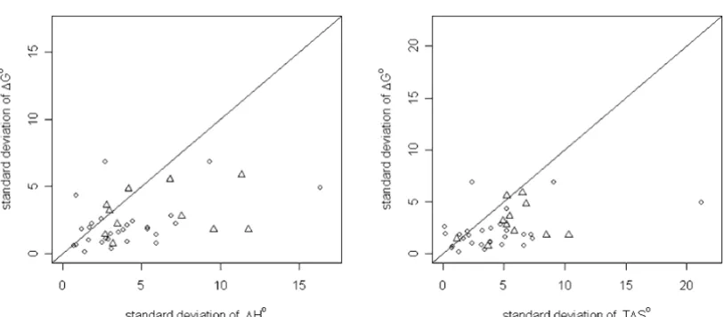
To further analyze these findings, we clustered the dataset compounds on the basis of their molecular similarity. Clusters were built using a similarity threshold of 0.7 with a complete linkage algorithm. In this way all structures within a cluster have a similarity of 0.7 or higher (see additional file 1: Table 2). We then calculated the mean values for ∆G°, ∆H° and T∆S° together with the standard deviations for all molecules within a cluster. Figure 5 shows the plot of the standard deviations of ∆G° against the corresponding standard deviations of ∆H° and T∆S°
within each cluster. In the majority of all cases, the points lie below the diagonal, indicating that the variance in the experimental ∆H° and T∆S° values is higher than the var-iance of the corresponding ∆G° values. This indicates the enthalpy and the entropy values' higher dependence on small structural changes in the ligand. This is nicely illus-trated, for example, by the calorimetrically-derived ther-modynamic data for inclusion complexes of a range of sulfonamides (additional file 1: Table 2 – Cluster ID 39), which were all found in one similarity cluster and studied within one laboratory. At ± 1.8 kJmol-1, the standard
devi-ation of the ∆G° values is relatively small. The corre-sponding standard deviations of ∆H° and T∆S°, however, are clearly higher, at ± 5.04 kJmol-1 and ± 3.84 kJmol-1,
respectively.
In addition, we attempted a nearest-neighbour prediction of ∆G°, ∆H° and T∆S° using the graph-based similarity of
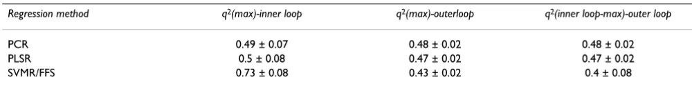
Table 2: Comparison of the regression methods for nested cross-validation (∆G°). Shown are the maximal q2 in the inner loop
(q2(max)-inner loop), the maximal q2 in the outer loop (q2(max)-outer loop) and the q2 of the outer loop predicted by the model with
the maximal q2 in the inner loop (q2 (inner loop-max)-outer loop).
Regression method q2(max)-inner loop q2(max)-outerloop q2(inner loop-max)-outer loop
PCR 0.71 ± 0.03 0.7 ± 0.03 0.69 ± 0.03
PLSR 0.71 ± 0.03 0.7 ± 0.01 0.69 ± 0.03
SVMR/FFS 0.87 ± 0.03 0.74 ± 0.01 0.71 ± 0.03
Table 3: Comparison of the regression methods for nested cross-validation (∆H°) with respect to q2. Shown are the maximal q2 in the
inner loop (q2(max)-inner loop), the maximal q2 in the outer loop (q2(max)-outer loop) and the q2 of the outer loop predicted by the
model with the maximal q2 in the inner loop (q2(inner loop-max)-outer loop).
Regression method q2(max)-inner loop q2(max)-outerloop q2(inner loop-max)-outer loop
PCR 0.49 ± 0.07 0.48 ± 0.02 0.48 ± 0.02
PLSR 0.5 ± 0.08 0.47 ± 0.02 0.47 ± 0.02
the molecules [31]. This method is independent of the E-Dragon descriptors [29] and regression methods. For each molecule within the dataset the three thermodynamic quantities were predicted to be equal to those of the most similar compound within the set. We obtained squared correlation coefficients r2 values of 0.50 for ∆G°, 0.47 for
∆H° and 0.29 for T∆S°. Except for a loss of accuracy in the prediction of ∆G°, the results are very similar to those obtained from the regression-based prediction. The main trend in the predictability of the thermodynamic quanti-ties observed in the regression analysis can also be observed in this analysis, where again T∆S° proves to be the least predictable thermodynamic parameter.
This analysis indicates that the lower ability to predict
T∆S° – and to a lesser extent, ∆H° – for different ligands has to do with the more complex dependence of T∆S° on even small structural changes in the ligand. This explana-tion is also consistent with the empirical observaexplana-tion of enthalpy-entropy compensation. The relative insensitivity of ∆G° to small structural changes compared to the other
two quantities would lead to the compensation effects in enthalpy and entropy according to ∆G° = ∆H°-T∆S°, and conversely, given entropy-enthalpy compensation, changes in entropy would lead to smaller changes in free energy.
Conclusion
In this study we investigated the predictability of three important thermodynamic quantities, namely, the free energy of binding, heat of formation and the entropy change upon binding. To this end, we chose β -cyclodex-trin with its ligands, a very well-studied system for which there is a large amount of high quality binding data avail-able. We were able to show that free energies of binding can be reliably predicted by means of simple, readily available molecular descriptors with all three of the linear regression methods studied. The SVMR/FFS method has the advantage of leading to a (partly) interpretable model with comparably few descriptors. However, in the applica-tion of SVMR/FFS it is important to perform a nested cross-validation in order to obtain a realistic impression of its generalisation ability. The predictability of ∆G°
obviously cannot be compared directly to that of ∆H°, as the latter is reproduced with significantly lower accuracy by the models analyzed. We found that T∆S° appears almost unpredictable, with an analysis of our results in the context of further data from the literature suggesting that its poor predictability – and, to a lesser extent, that of ∆H° – is explained by a stronger dependence of those quantities on the complex's structural details, and to a lesser extent on the wider experimental error. This would also explain the well-documented empirical finding of entropy-enthalpy compensation. In this sense our conclu-sion is in disagreement with that of Sharp, which sug-gested that entropy-enthalpy compensation is most likely due to lower accuracy in the experimental determination of binding enthalpy and entropy.
Methods
Dataset choice and preparation of the molecules
We assembled a dataset consisting of 176 β-CD ligands (see additional file 1; Table 1). These molecules are a sub-set of those collected by Rekharsky et al [23]. We applied the following selection criteria:
Enthalpy-entropy compensation
Figure 4
Enthalpy-entropy compensation.
Table 4: Comparison of the regression methods for nested cross-validation (T∆S°) with respect to q2. Shown are the maximal q2 in the
inner loop (q2(max)-inner loop), the maximal q2 in the outer loop (q2(max)-outer loop) and the q2 of the outer loop predicted by the
model with the maximal q2 in the inner loop (q2(inner loop-max)-outer loop).
Regression method q2(max)-inner loop q2(max)-outerloop q2(inner loop-max)-outer loop
PCR 0.33 ± 0.09 0.3 ± 0.05 0.3 ± 0.03
PLSR 0.32 ± 0.1 0.29 ± 0.04 0.29 ± 0.04
• The availability of experimental data derived from either calorimetric (cal) or UV-spectroscopic measurements;
• The availability of ∆G°, ∆H° and T∆S° data;
• The exclusion of all guest molecules whose data deviated from measurements of other groups.
We drew two-dimensional Lewis structures of the mole-cules with ISIS-Draw and exported them as MDL MOL files [24]. The protonation state of each molecule was manually set according to the pH value at which the meas-urement was performed. When no pH data were available, a reasonable state was set. To generate three dimensional low-energy structures from the mol file we used CORINA [25]. We then converted the structures to SD-files [26]. Finally, all structures were manually inspected and, when needed, corrected.
Calculation and processing of molecular descriptors We calculated molecular descriptors for all molecules using the web service E-Dragon, which is part of the Vir-tual Computational Chemistry Laboratory [27,28]. E-Dragon can calculate up to 1,666 different molecular descriptors [29], which are grouped into different catego-ries ranging from simple atom-type descriptors or frag-ment counts to more sophisticated topological, geometrical or quantum chemical descriptors. In order to
prevent numerical problems and to ensure the avoidance of any bias in the descriptor space, we normalised all descriptor values to a range between -1 and +1.
Regression Methods
The statistical methods used in this work have been employed on numerous occasions elsewhere. For PCR and Partial PLSR the R-package PLS was used [14]. The support vector machine regression was performed with LIBSVM, which was developed by Chang et al [30].
Principal component regression
In PCR a multiple linear regression is performed on prin-cipal components. Prinprin-cipal components are linear com-binations of the descriptors in the data matrix and explain their variance. They are derived from the covariance matrix of the calculated descriptors. The number of prin-cipal components corresponds to the data matrix rank. Its maximal value is the minimum of the number of data points (i.e. molecules) and descriptors.
The first principal component of a data matrix points in the direction that maximizes the variance of the descrip-tors and corresponds to the largest eigenvalue of the cov-ariance matrix. The second corresponds to the second largest eigenvalue and points in the direction that maxi-mizes the variance and is orthogonal to the first principal component, and so on for the remaining principal
com-Plot of the standard deviations of ∆G° against the standard deviations of ∆H° (left side) and T∆S° (right side) for each cluster
Figure 5
ponents. The PCR model is generated on a subset of the components. The subset is built by selecting the compo-nents in the order of their ability to explain the variance in the dependent variable, i.e. in this study, the thermody-namic properties.
Partial Least Squares Regression
PLSR is very similar to PCR, however, while the covariance matrix of the data is used to generate the principal compo-nents, in PLSR the principal components are derived from the cross-covariance between the data matrix and the dependent variables. Hence, while in PCR the eigenvec-tors of the data covariance matrix are used to span the solution space, in PLSR the directions of maximal covari-ance between data and the dependent variables are used.
Support vector machine regression combined with forward feature selection
The theoretical background of support vector machine regression has been described in detail by Drucker et al
[15]. Support vector regression is a straightforward variant of support vector machine (SVM) classification [16]. In classification problems SVMs find the hyper plane that separates positive examples from negative examples with a maximum margin (where the margin is defined as the distance of the closest data point from the separating hyper plane). In this way a statistical model is produced that only depends on a subset of the training data, namely those data points that are close enough to influence the size of the margin and the orientation of the hyper plane. These are the most difficult examples in the training set. They are termed 'support vectors' because they define the orientation of the separating plane. In support vector regression (SVMR) the same effect (namely that the final model depends only on a subset of the data) is achieved by the use of a so-called 'ε-insensitive cost function', which during model optimization ignores errors up to a defined threshold. This means that any training data being predicted by the current model with an accuracy of up to εcan be neglected.
In this work we added a 'forward feature selection proce-dure', which is in some respects similar to the component extension in PCR and PLSR. Forward feature selection increases the learning performance and the interpretabil-ity of the regression model as only descriptors are selected that significantly improve the SVMR model. The selection of descriptors produces combinatorial explosion if all possible subsets of all the available descriptors have to be considered. This, of course, is not feasible if the number of descriptors is too large. To overcome this problem, for-ward feature selection uses the following greedy heuristic, that is, for each single descriptor a support vector regres-sion model is trained with tenfold cross-validation. The descriptor leading to the model with the highest q2 value
is selected as the start descriptor. The procedure is repeated to find the next descriptor to form the best pair, triplet etc., iteratively expanding the model by one descriptor until q2 reaches a maximum, at which point the
final model is obtained.
Validation by means of nested cross-validation
In order to validate whether our model generation proce-dures can lead to a predictive model that provides reliable output, we performed a nested three-way cross-validation protocol as proposed by Ruschhaupt et al [20] for each of the regression methods. To this end, we first split the training set into three equally sized subsets by randomly assigning training dataset molecules to one of the subsets (S1 and S2 consist of 59 molecules, S3 consists of 58
mole-cules). We then generated three validation sets, each as a combination of two subsets (V1→ S1 and S2, V2→ S1 and S3, V3→ S2 and S3), such that each of the validation sets could be used as a training-set for predicting the binding energies of the remaining subset (test set) that is not included in the respective training set. A ten-fold cross val-idation is used within the valval-idation set (e.g. V1) to iden-tify the optimal model (e.g. the number of components in PCR/PLS or descriptors in SVMR), meaning that V1 is again separated into ten subsets that are used for cross val-idation in a ten-fold loop. The model resulting from this inner loop is then used to predict the test set (e.g. S3). This is performed once for every validation set/test set combi-nation, three times in total. Thus the reported results on the test sets from the outer loop do not in any way influ-ence the choice of model parameters and are comparable to independent test set validations. The advantage of this approach over independent test set validation, is that every data point is predicted once in one of the three test sets, thus reducing the effects of test set choice.
Calculation of molecular similarity and clustering of the molecules
To cluster the dataset molecules and for the nearest-neigh-bour prediction, we calculated all pair-wise molecular similarities using our in-house similarity tool GMA [31]. The molecular similarity was calculated on the basis of a graph-based alignment. The better the molecular graphs (i.e. the topology and the atom types) of two molecules can be matched, the greater the similarity between these two molecules (1 = identical, 0 = dissimilar). On the basis of these similarities we performed complete-linkage hier-archical clustering. The cluster tree was cut off at a similar-ity threshold of 0.7. Hence, within one cluster only those molecules that exhibit a similarity of 0.7 or higher are grouped (see additional file 1, Table 2).
Authors' contributions
Open access provides opportunities to our colleagues in other parts of the globe, by allowing
anyone to view the content free of charge.
Publish with
Chemistry
Central and every
scientist can read your work free of charge
W. Jeffery Hurst, The Hershey Company.
available free of charge to the entire scientific community peer reviewed and published immediately upon acceptance cited in PubMed and archived on PubMed Central yours you keep the copyright
Submit your manuscript here:
http://www.chemistrycentral.com/manuscript/
Additional material
Acknowledgements
We are grateful to Deutsche Forschungsgemeinschaft for funding part of this work (grants AP-101/1 and KA-1804/1). The authors wish to thank Joachim Büch for technical support, and Thomas Lengauer for critically reading an early version of the manuscript.
References
1. Wenz G: Cyclodextrins As Building-Blocks For Supramolecu-lar Structures And Functional Units. Angew Chem-Int Edit Engl
1994, 33(8):803-822.
2. Muller A, Wenz G: Thickness recognition of bolaamphiphiles by alpha-cyclodextrin. Chemistry 2007, 13(8):2218-2223. 3. Davis ME, Brewster ME: Cyclodextrin-based pharmaceutics:
past, present and future. Nat Rev Drug Discov 2004, 3:1023-1035. 4. Fugen G, Cuijing L: The preparation of inclusion compound of diclofenac sodium-[beta]- cyclodextrin. Chinese Pharmaceutical Journal 1998, 33(3):153.
5. Kang JC, Kumar V, Yang D, Chowdhury PR, Hohl RJ: Cyclodextrin complexation: influence on the solubility, stability, and cyto-toxicity of camptothecin, an antineoplastic agent. Eur J Pharm Sci 2002, 15(2):163-170.
6. Stanton J, Vincent P: Tumor necrosis factor receptor 2 . USA , Nuvelo, Inc.; 2001.
7. Stuerzebecher CS, Witt W, Raduechel B, Skuballa W, Vorbrueggen H: Prostacyclins, their analogs or prostaglandins and boxane antagonists for treatment of thrombotic and throm-boembolic syndromes. USA , Schering Aktiengeselleschaft; 1996. 8. Szejtli J, Bolla-Pusztai E, Szabo P, Ferenczy T: Enhancement of sta-bility and biological effect on cholecalciferol by beta-cyclo-dextrin complexation. Pharmazie 1980, 35(12):779-787. 9. Connors KA: Prediction of binding constants of
alpha-cyclo-dextrin complexes. J Pharm Sci 1996, 85(8):796-802.
10. Lipkowitz KB: Applications of computational chemistry to the study of cyclodextrins. Chem Rev 1998, 98(5):1829-1873. 11. Suzuki T: A nonlinear group contribution method for
predict-ing the free energies of inclusion complexation of organic molecules with alpha- and beta-cyclodextrins. J Chem Inf Com-put Sci 2001, 41(5):1266-1273.
12. Katritzky AR, Fara DC, Yang HF, Karelson M, Suzuki T, Solov'ev VP, Varnek A: Quantitative structure-property relationship mod-eling of beta-cyclodextrin complexation free energies. J Chem Inf Comput Sci 2004, 44(2):529-541.
13. Liu L, Guo QX: Wavelet neural network and its application to the inclusion of beta-cyclodextrin with benzene derivatives.
Journal Of Chemical Information And Computer Sciences 1999,
39(1):133-138.
14. Mevik RWBH: pls: Partial Least Squares Regression (PLSR) and Principal Component Regression (PCR). R package ver-sion 2.0-1 edition. 2007 [http://mevik.net/work/software/pls.html]. 15. Drucker H, Burges CJC, Kaufman L, Smola A, Vapnik V: Support
Vector Regression Machines. Volume 9. MIT Press; 1996:155-161. 16. Cortes C, Vapnik V: Support-Vector Networks. Machine Learning
1995, 20(3):273-297.
17. Briem H, Gunther J: Classifying "kinase inhibitor-likeness" by using machine-learning methods. Chembiochem 2005,
6(3):558-566.
18. Liu X, Lu WC, Jin SL, Li YW, Chen NY: Support vector regression applied to materials optimization of sialon ceramics. Chem-ometr Intell Lab Sys 2006, 82(1-2):8-14.
19. Jorissen RN, Gilson MK: Virtual screening of molecular data-bases using a Support Vector Machine. J Chem Inf Model 2005,
45(3):549-561.
20. Ruschhaupt M, Huber W, Poustka A, Mansmann U: A Compen-dium to Ensure Computational Reproducibility in High-Dimensional Classification Tasks. Statistical Applications in Genet-ics and Molecular Biology 2004.
21. Sharp K: Entropy-enthalpy compensation: fact or artifact? Pro-tein Sci 2001, 10(3):661-667.
22. Ross PD, Rekharsky MV: Thermodynamics of hydrogen bond and hydrophobic interactions in cyclodextrin complexes. Bio-phys J 1996, 71(4):2144-2154.
23. Rekharsky MV, Inoue Y: Complexation Thermodynamics of Cyclodextrins. Chem Rev 1998, 98(5):1875-1918.
24. MDL Information Systems I: MDL ISIS/Draw. 2.5th edition. MDL Information Systems, Inc. . 1990-2002
25. Sadowski J, Gasteiger J: From Atoms and Bonds to Three-Dimensional Atomic Coordinates: Automatic Model Build-ers. Chem Rev 1993, 93:2567-2581.
26. Dalby A, Nourse JG, Hounshell WD, Gushurst AKI, Grier DL, Leland BA, Laufer J: Description of several chemical structure file for-mats used by computer programs developed at Molecular Design Limited. J Chem Inf Comput Sci 1992, 32(3):244-255. 27. Tetko IV, Gasteiger J, Todeschini R, Mauri A, Livingstone D, Ertl P,
Palyulin V, Radchenko E, Zefirov NS, Makarenko AS, Tanchuk VY, Prokopenko VV: Virtual computational chemistry laboratory -design and description. J Comput-Aided Mol Des 2005,
19(6):453-463.
28. Tetko IV: Computing chemistry on the web. Drug Discov Today
2005, 10(22):1497-1500.
29. Todeschini R, Consonni V: Handbook of Molecular Descriptors.
In Methods and Principles in Medicinal ChemistryVolume 11. Edited by: Mannhold R, Kubyini H, Timmermann H. Weinheim , Wiley-VCH; 2000.
30. Chang CC, Lin CJ: LIBSVM : a library for support vector machines . 2001.
31. Marialke J, Korner R, Tietze S, Apostolakis J: Graph-Based Molec-ular Alignment (GMA). J Chem Inf Model 2007, 47(2):591-601.
Additional file 1
Contains two tables with all the data used in this study (Table 1) and a list of the clusters' average properties according to structural similarity (Table 2).
Click here for file