Analysis of a Krylov subspace enhanced parareal algorithm for linear problems

E. Canc`es, S. Faure, B. Graille, Editors

ANALYSIS OF A KRYLOV SUBSPACE ENHANCED PARAREAL

ALGORITHM FOR LINEAR PROBLEMS

M. Gander

and M. Petcu

Abstract. The parareal algorithm is a numerical method to integrate evolution prob-lems on parallel computers. The performance of the algorithm is well understood for diffusive problems, and it can have spectacular performance when applied to certain non-linear problems. Its convergence properties are however less favorable for hyperbolic problems. We present and analyze in this paper a variant of the parareal algorithm, re-cently proposed in the PITA framework for systems of second order ordinary differential equations.

1.

_Introduction

The parareal algorithm is a time parallel time integration method for evolution problems intro-duced by Lions, Maday and Turinici in [6]. It can be used to compute in parallel an approximate solution of systems of ordinary differential equations (ODEs). The method was introduced in or-der to obtain a speed-up on parallel computers when solving evolution problems, which need to be solved in real time, which explains its name. The advantage of this method, as shown in [6], is that it approximates the solution later in time, before having fully accurate approximations at earlier times, while the global accuracy of the iterative process after few iterations is comparable to that given by a sequential method used on a fine discretization in time.

The method has received great attention over the last years, and it was used for different applications in financial mathematics (see e.g. [1]) in robotics, biology and engineering (see [2]), as well as in quantum chemistry (see [7]). The parareal algorithm was also written in different forms: by Farhat and Chandesris (see [2]) as an algorithm called PITA (Parallel Implicit Time Integrator), and by Gander and Vanderwalle (see [5]) as a multiple shooting method. Gander and Vandewalle showed in [5] that the parareal algorithm is a multiple shooting method for initial value problems with a coarse grid approximation for the Jacobian in Newtons method. They also proved that when the method is applied to linear, diffusive problems, it converges linearly on long time intervals and super-linearly on short time intervals. In [4], [1], [2], the authors showed that the parareal algorithm produces a speed-up for first order ODEs, but the method does not have the

1 _{Section de Math´ematiques, University of Geneva, Switzerland} 2 _{Laboratoire de Math´ematiques, Universit´e de Poitiers, France}

The Institute of Mathematics of the Romanian Academy, Bucharest, Romania c

EDP Sciences, SMAI 2008

same potential for second order ODEs, see also [5]. In [3], the authors proposed a method in order to adapt the existing PITA algorithm to second order differential equations.

This paper is structured in two parts: in the first part we introduce the parareal algorithm as a multiple shooting method and recall the existing convergence analysis for this method. In the second part, we introduce the modified algorithm, explain the reason for which this method gives better results for systems of linear ODEs, and prove convergence results similar to the ones for the original method.

2.

_{Parareal algorithm as a multiple shooting method}

The parareal algorithm is a time parallel method to compute in parallel the solution of the system of ODEs

u0_{(t) =f(u(t)), t∈(0, T), u(0) =u}

0, (2.1)

wheref :Rd_→Rd _andu:R→Rd_.

The parareal algorithm is described by Gander and Vandewalle [5] as a multiple shooting method

with the use of two propagation operators. The inexpensive coarse propagatorG(Tn, Tn−1, x) gives

a rough approximation to u(Tn), where u is the solution of equation (2.1) having u(Tn−1) =x

as initial condition, while the expensive fine propagator F(Tn, Tn−1, x) gives a more accurate

approximation to the same u(Tn). Partitioning the time domain (0, T) intoN-time subdomains

Ωn= (Tn, Tn+1), the algorithm works as follows:

• Step 0: The algorithm starts with an initial approximationU0

n, n= 0, . . . , N, which can be found for example using the coarse propagator sequentially,

Un0+1=G(Tn+1, Tn, Un0), U00=u0. (2.2)

• Stepk+ 1: We perform a correction step, using both the coarse and fine propagator,

Uk+1

n+1=G(Tn+1, Tn, Unk+1) +F(Tn+1, Tn, Unk)−G(Tn+1, Tn, Unk). (2.3)

We note that the initial step (2.2) of the algorithm is sequential, but not expensive, since we use the

coarse and cheapG-propagator. In the iteration (2.3), the approximations can potentially become

better since we improve the accuracy with the aid of theF-propagator. A significant advantage

of the method is that since we already know the valuesUk

n, for alln, the expensive computations

forF(Tn+1, Tn, Unk) can be performed in parallel and (2.3) is reduced to a sequential computation

with cost comparable toG(Tn+1, Tn, Unk+1).

We now recall a convergence result proved in [4], where it was assumed for simplicity that

the fine propagatorF is the exact solution of the problem, and equal time subdomains are used,

Tn+1 −Tn = 4T. Furthermore, it was assumed that the difference between the approximate

solution given by the coarse propagatorGand the exact solution satisfies the relation

F(Tn, Tn−1, x)−G(Tn, Tn−1, x) =cp+1(x)∆Tp+1+cp+2(x)∆Tp+2+. . . , (2.4)

where the coefficientscjwithj=p+1, p+2, . . .are continuously differentiable, and thatGsatisfies

the Lipschitz condition

Theorem 2.1. Under the conditions above, the erroru(Tn)−Unkat stepkof the parareal algorithm

satisfies the convergence estimate

|u(Tn)−Unk| ≤C1

(∆Tp+1₎k+1

(k+ 1)! (1 +C2∆T)

n−k−1

k

Y

j=0

(n−j)

≤C1 Tnk+1

(k+ 1)!expC2(Tn−Tk+1)4T

p(k+1)_,

(2.6)

whereC1 is a constant depending on the coefficients in (2.4), andC2 is the constant in (2.5).

3.

_{PITA algorithm and equivalence to the parareal algorithm}

We now present the PITA algorithm introduced by Farhat et al. in [2], and prove that for linear problems the algorithm is equivalent to the multiple shooting method. We consider the linear system of first order ODEs

u0_{(t) =Au(t) +b(t), (3.1)}

withA∈ Md(R) andb(·)∈Rd.

The time interval [0, T] is partitioned intoN time subdomains Ωnof constant size ∆T, obtaining

this way a coarse grid. Each time subdomain is then partitioned in turn intoJ subintervals of size

∆t, obtaining a fine grid. Then the PITA algorithm is given by

• Step 0: Provide an initial approximate solutionU0

n,n= 0, . . . , N by applying a sequential numerical method to problem (3.1) on the coarse grid.

• Stepk+ 1:

– Using the available approximate solution Uk

n as initial condition for problem (3.1)

considered on each time slice, apply a sequential numerical method on the decomposed fine grid,

(ukn)0(t) =Au

k

n(t) +b(t), on Ωn,

uk

n(Tn) =Unk.

(3.2)

Note that the computations (3.2) can be done in parallel for each time slice.

– Evaluate the jumps

Sk

n=u

k

n−1(Tn)−Unk, 1≤n≤N, (3.3)

on the coarse grid. If the jumps are small enough, the algorithm terminates.

– Solve, by the numerical method applied on the coarse grid, sequentially the correction

problem

(ck

n)

0_{(t) =Ac}k

n(t), c

k

0(T0) = 0, ckn(Tn) =ckn−1(Tn) +Snk, (3.4)

and compute the correctionCk

n=ckn−1(Tn).

– Update the approximate solution using the formula

Uk+1

n =u

k

n−1(Tn) +Cnk =U

k

n+S

k

n+C

k

Proposition 3.1. For the linear problem (3.1), the PITA algorithm described above is equivalent to the multiple shooting algorithm (2.2), (2.3).

Proof. We first note that the fine propagator of the multiple shooting method corresponds to applying a sequential numerical method on the fine grid, while the coarse propagator corresponds to applying a sequential numerical method on the coarse grid. Clearly the initial step is then the same for both methods. Rewriting the PITA method using the propagators, we find that the jumps are

Snk =F(Tn, Tn−1, Unk−1)−Unk. Since we propagate the jumps on the coarse grid, the corrections are

Ck

n+1=G(Tn+1, Tn, Cnk+S

k

n)−G(Tn+1, Tn,0). (3.6)

Using the updating formula (3.5), we obtain

Uk+1

n =u

k

n−1(Tn) +Cnk=U

k

n+S

k

n+C

k n,

which implies that

Sk

n+Cnk =Unk+1−Unk. (3.7)

Rewriting the updating formula (3.5) using the fine propagator, we find with the expression for the correction (3.6), relation (3.7), and using linearity

Unk+1+1=F(Tn+1, Tn, Unk) +C k

n+1

=F(Tn+1, Tn, Unk) +G(Tn+1, Tn, Cnk+S

k

n)−G(Tn+1, Tn,0)

=F(Tn+1, Tn, Unk) +G(Tn+1, Tn, Unk+1−U

k

n)−G(Tn+1, Tn,0)

=F(Tn+1, Tn, Unk) +G(Tn+1, Tn, Unk+1)−G(Tn+1, Tn, Unk),

which coincides with the updating formula (2.3) of the multiple shooting algorithm.

When the parareal algorithm is applied to the system of second order ODEs

M q00_+Dq0_{+Kq=f(t), q(T}

0) =q0, q0(T0) =q00, (3.8)

whereM, D, K ∈ Md,˜d˜(R) represent respectively the mass, the damping and the stiffness matrices,

the algorithm does not perform well, because of a beating phenomenon, see [3]. In order to understand this, we rewrite equation (3.8) in the homogeneous case as a system of first order ODEs, assuming that the mass matrix is invertible, and obtain

u0=Au, u(T0) =u0, (3.9)

where the matrixA∈ Md,d(R) is given by

−M−1_{D −M}−1_K

Id O

,

and u0 = (q00, q0)0 ∈Rd, with d= 2 ˜d. Now the exact solution of the problem can be expressed

system, i.e. the eigenvalues of matrixA, which are purely imaginary numbers. When we compute the approximate solution using formula (2.3), we can have a beating phenomenon caused by the interference of two modes not having the same frequencies,

F(Tn+1, Tn, φi) =eiαiφi,

withαi a constant depending on the eigenvalues of the matrixAand on the time-step ∆T, andφi

a natural mode of the problem. Suppose thatαandβ are two natural frequencies that appear in

Uk+1

n andUnk. Then, when we computeUnk+1−Unk we find that this difference is characterized by

the frequencies (α+β)/2 and (α−β)/2. Ifαandβ are frequencies close to each other, the order of

the new frequency (α−β)/2 becomes very small and the frequency (α+β)/2 becomes very close

to the natural frequenciesαandβ and while computingG(Tn+1, Tn, Unk+1)−G(Tn+1, Tn, Unk) the

result might not be accurate unless ∆T is very small.

4.

_{Krylov subspace enhanced parareal algorithm}

In [1], [2] and [3], the authors showed that the parareal algorithm produces a speed-up for certain first order ODEs, but the method does not have the same potential when applied to systems of second order ODEs. It was also shown in [1], as well as in [8] that the parareal algorithm is not stable for certain second order ODEs (in fact the method is unstable when the system presents purely imaginary eigenvalues) or for most hyperbolic problems (since the situation of purely complex eigenvalues or complex eigenvalues with large imaginary part appears). We propose and analyze here a modified parareal algorithm, based on an idea presented in the PITA framework in [3] as a remedy for a beating phenomenon when the algorithm is applied to a system of second order ODEs. We consider the inhomogeneous linear system of first order ODEs

u0_{(t) =Au(t) +f(t), u(T}

0) =u0, (4.1)

whereA∈ Md,d(R),f :R→Rd andu:R→Rd.

4.1.

Homogeneous case

We start by considering the homogeneous case; we will see later that the inhomogeneous case can also be treated in a similar manner. In the correction step (2.3) of the original parareal algorithm, the fine propagator is used for every time subdomain, and if the equation is linear and homogeneous, one knows by linearity rapidly the evolution of the solution for a larger and larger subspace of initial conditions. This information can be used to obtain a more accurate

approximation for the coarse propagatorGwhen we computeG(Tn+1, Tn, Unk+1−Unk) in (2.3) (we

used linearity), at no extra cost. The idea is to use the fine propagatorF for the part ofUk+1

n −Unk

in the subspace for which the evolution is already known from previous evaluations of the fine propagator, and to only propagate the rest with the coarse propagator. More formally, we define the space

Sk= span{Unl; 0≤l≤k, 0≤n≤N}, (4.2)

and replace in (2.3) the coarse propagation G(Tn+1, Tn, Y) by K(Tn+1, Tn, Y), where the new

propagatorKis defined by

andPk _{is the orthogonal projection onto the spaceS}k_,

Pk _=Sk_(Sk₎T_{. (4.4)}

Introducing this into (2.3), we obtain by linearity after simplification the modified update

Unk+1+1 =F(Tn+1, Tn, PkUnk+1) +G(Tn+1, Tn,(I−Pk)Unk+1). (4.5)

Note that if we formally takek→ ∞in (4.5), we have that the projectionPk tends to the identity

and soUk+1

n tends to the approximate solution given by the fine propagator. A rigorous explanation

for the fact thatPktends to the identity when the algorithm converges can be found in Remark 4.2

where we show that we converge when the spaces{Sk}k do not increase anymore.

The modified parareal algorithm computes this update performing the following steps:

• Step 0: As for the original parareal algorithm, we start with the initial approximationsU0

n

from (2.2), and the initial subspaceS−1_{is empty, since we have done no evaluation of the}

fine propagatorF.

• Stepk+ 1:

– Compute in parallelF(Tn+1, Tn, Unk).

– We enhance the subspace of known fine evolution by

Sk_{= span(S}k−1_{∪ {U}k

n, n= 0, . . . , N}), (4.6)

since now the fine evolution for all initial conditionsUk

n is known. We also construct an

orthogonal basis forSk_{, whose columns we store in the matrixS}k_{, and the associated}

orthogonal projectorPk _{using (4.4).}

– We perform the sequential updating step (4.5) forn= 0, . . . , N, at no extra evaluation

of the fine propagator, since the fine evolution on the subspaceSk _{is known.}

4.2.

Properties of the subspaces

S

Initially, the matrixS0 _{contains as columns the linearly independent vectors that generate}

S0_{= span(U}0

n; 0≤n≤N).

In the algorithm, the vectorsU0

n are found using the coarse propagatorG,

U0

n =G(Tn, Tn−1, Un0−1) =GUn0−1, U00=U0,

where we use the same symbol G for the matrix that defines the coarse propagator G in the

homogeneous linear case under consideration. We therefore obtain that

S0=KN+1(U0, G), (4.7)

whereKN+1(U0, G) is a Krylov space. Therefore, the dimension of S0 is given by

p:= dimKN+1(U0, G) = min(N+ 1,grade(U0)), (4.8)

where grade(U0) is the degree of the minimal polynomial ofGwith respect toU0. It is then well

known that

and hence the matrixS0 _{contains as columns the orthonormalized vectorsU}

0, U10, . . . , Up0−1.

Proposition 4.1. If the matrix G has only simple eigenvalues, then the degree pof the matrix G with respect to the vectorU0 coincides with the number of natural modes excited by the initial condition.

Proof. Letφi, i= 1, . . . , N be the natural modes of the system (3.9), i.e. the eigenvectors of the

matrixA. One can easily see that the matricesA and Ghave the same eigenvectors. Let λi be

the eigenvalues of Gcorresponding to the eigenvectorsφi, and suppose that the initial condition

can be written in the form

U0=β1φ1+. . .+βlφl, withβi6= 0 fori= 1,2, . . . , l.

We know that the grade ofGwith respect toU0is the smallest degree of a polynomialpsuch that

p(G)U0= 0. Since

p(G)U0=β1p(G)φ1+. . .+βlp(G)φl=β1p(λ1)φ1+. . .+βlp(λl)φl= 0, (4.9)

and taking into account the linear independence of the eigenvectors and the fact that all the

coefficientsβi are nonzero, we must havep(λi) = 0 for alli= 1, . . . , l. Thus the smallest degree of

the polynomial isl, the number of natural modes excited by the initial conditionU0.

After this initial step, the algorithm enhances at each step the subspaceSk−1 _{with the vectors}

obtained from the current step, Uk

0, . . . , UNk. If the matrix Sk−1 is known from the previous

iteration, we can construct the new matrix Sk _{for example by using modified Gram-Schmidt to}

form the extended orthogonal basis, or QR factorization steps.

Remark 4.2. The structure of the spaceS0_{is quite simple, as we have seen before. Fork≥1 the}

spacesSk_{are much more complicated. To see why, we just give a simple example: consider in what}

follows that both the coarse and the fine propagators are obtained using the Euler method

respec-tively on a coarse and fine grid. Then, F = (I+ ∆tA)J _{and G=I+ ∆T A. The approximations}

at Step 0 areU0

k = (1 + ∆T A)

k _{and the spaceS}0 _is:

S0= span{U00, . . . , UN0}= span{U0, AU0, . . . , ANU0}.

In order to find S1, we need to first compute the approximations at Step 1. It can be easily

seen that U1

0 = U0 and, since U0 ∈ S0, we find U11 = F(T1, T0, P0U01) = (I + ∆tA)JU0 and

U1

2 =F(T2, T1, P0U11) +G(T2, T1,(I −P0)U11). To further compute U21 we need to know ifU11 is

an element of S0_{. If so (case possible if for example J ≤dim(S}0_{)) then U}1

2 = (I+ ∆tA)2JU0; if

not, we need to project U1

1 into the space S0, use the fine projector for the part P0U11 and the

coarse projector for the remaining part. So, the approximations at Stepkare linear combinations

of vectors of the formAl_U

0, butl will in general be from a non-contiguous subset ofN, and thus

form a “broken” Krylov space, in contrast to the case at Step 0.

4.3.

Inhomogeneous case

propagator for a linear inhomogeneous problem can be decomposed by linearity into

F(Tn+1, Tn, αX+βY) =FJ(αX+βY) +F(Tn+1, Tn,0)

=αFJX+βFJY +F(Tn+1, Tn,0)

=α(F(Tn+1, Tn, X)−F(Tn+1, Tn,0))

+β(F(Tn+1, Tn, Y)−F(Tn+1, Tn,0)) +F(Tn+1, Tn,0),

whereFis the matrix that defines the fine propagator. The affine computation forF(Tn+1, Tn, PkUnk+1),

and similarly forG(Tn+1, Tn, PkUnk+1), requires thus an additional preprocessing step, which leads

to the algorithm:

• Step -1: We start the algorithm by computing the quantitiesF(Tn+1, Tn,0) andG(Tn+1, Tn,0).

The utility of these terms is seen at Stepk+ 1 when we need to update the approximation.

• Step 0: At this step we are doing the same computations as for the homogeneous case, in

order to obtain initial approximationsU0

n. Also the initial subspaceS−1is empty.

• Step (k+ 1):

– Compute in parallelF(Tn+1, Tn, Unk).

– Enhance the subspace of known fine evolution by

Sk= span(Sk−1_{∪ {U}k

n, n= 0, . . . , N}),

as in the homogeneous case, and compute the matrixSk _{and the projectorP}k_.

– Update the approximate solution using the formula

Uk+1

n+1 =F(Tn+1, Tn, PkUnk+1) +G(Tn+1, Tn,(I−Pk)Unk+1)−G(Tn+1, Tn,0). (4.10)

Note here that if we formally takek→ ∞in (4.10), we find thatPk tends toI and soUnk+1+1 tends

to the fine solution. The last term in (4.10) was zero for the homogeneous case, here it is not zero

but it is a term that was computed at Step−1.

We also note that at Step k+ 1 the term F(Tn+1, Tn, PkUnk+1) can be computed at minimal

cost, since PkUnk+1 is a linear combination of approximations for which the evolution is known.

In fact,F(Tn+1, Tn, PkUnk+1) is computed as a linear combination of F(Tn+1, Tn,0) computed at

Step−1 and ofF(Tn+1, Tn, Sk),

F(Tn+1, Tn, PkUnk+1) = [F(Tn+1, Tn, Sk)−F(Tn+1, Tn,0)](Sk)TUnk+1+F(Tn+1, Tn,0),

where byF(Tn+1, Tn, Sk) we understand the matrix having as columns the evolution by the fine

propagator F of the column vectors of the matrix Sk_{, and F(T}

n+1, Tn,0) is the matrix of the

same dimension asSk_{, having as columns the vectorF(T}

n+1, Tn,0). The matrix F(Tn+1, Tn, Sk)

is known once we computed in parallel the evolution of Uk

n using the fine propagator: ifU is the

matrix of all the generators ofSk_{, we compute (or update) the QR factorization ofU (U =QR),}

and we simply compute

4.4.

Modified PITA algorithm and equivalence with the Krylov enhanced parareal

algorithm

The idea of modifying the multiple shooting method in order to be effective for second order ODEs came from [3], where the authors proposed a modified PITA algorithm. In what follows, we describe the modified PITA algorithm and we show that the two methods are equivalent for linear problems. We denote for the new PITA method the amplification matrices of a given sequential

numerical method associated with the coarse and fine time-grids by GandF respectively. Then,

the new PITA method works as follows:

• Step 0: Provide an initial approximate solutionU0

nwith 0≤n≤Nby applying a numerical

method to problem (3.1) on the coarse grid.

• Stepk+ 1:

– Using the available approximate solution Uk

n, n = 0, . . . , N as initial condition for problem (3.1) considered on each time slice, apply a sequential numerical method on the decomposed fine grid:

(ukn) 0

(t) =Aukn(t) +b(t), on Ωn,

uk

n(Tn) =Unk.

(4.11)

We note that the computations (4.11) can be done in parallel for each time slice.

– Evaluate the jumps:

Snk=u k

n−1(Tn)−Unk, 1≤n≤N, (4.12)

on the coarse grid. If the jumps are small enough, we terminate the algorithm.

– Construct the space Sk _{and the corresponding projection P}k _{(same definition as in}

(4.2) and (4.4)).

– Compute the correction propagating the jump on both the coarse and fine time-grids:

Ck

0 = 0, Cnk+1= (F

J

Pk+G(I−Pk))(Cnk+S k n),

(4.13)

with 0≤n≤N−1.

– Update the approximate solution:

Uk+1

n =u

k

n−1(Tn) +Cnk =U

k

n+S

k

n+C

k

n, for all 1≤n≤N. (4.14)

Proposition 4.3. For linear problems, the modified PITA algorithm described above is equivalent to the modified multiple shooting algorithm proposed.

Proof. We first note that for the linear case, the fine propagator of the multiple shooting method

can be written in terms of the amplification matrixF,

F(Tn, Tn−1, Y) =FJY +F(Tn, Tn−1,0),

and the coarse propagator can be written in terms of the amplification matrixG,

The corrections can therefore be written in the form

Ck

0 = 0, Ck

n+1= (FJPk+G(I−Pk))(Cnk+Snk)

=F(Tn+1, Tn, Pk(Cnk+S

k

n))−F(Tn, Tn−1,0)

+G(Tn+1, Tn,(I−Pk)(Cnk+Snk))−G(Tn, Tn−1,0).

Since we know that Sk

n+Cnk =Unk+1−Unk, we find that the updated solution is

Unk+1+1 =F(Tn+1, Tn, Unk) +F(Tn+1, Tn, Pk(Unk+1−U k

n))−F(Tn, Tn−1,0)

+G(Tn+1, Tn,(I−Pk)(Unk+1−U

k

n))−G(Tn, Tn−1,0)

=F(Tn+1, Tn, PkUnk+1) +G(Tn+1, Tn,(I−Pk)Unk+1),

where we used the fact that Pk_Uk

n =Unk. We thus obtained the same formula for updating the

approximate solution in the PITA algorithm as for the modified multiple shooting method.

5.

_{Mathematical analysis}

In [3], the authors have already shown for the modified PITA algorithm that when choosing two

p-th order sequential coarse and fine numerical methods, then the algorithm converges in a finite

number of steps and the algorithm preserves the accuracy of the fine numerical method. We present now a refined convergence analysis for the new parareal algorithm. For simplicity, we consider the homogeneous case only, the proofs for the inhomogeneous case follow the same ideas. In what

follows, we assume that the initial condition excitesl-natural modes, i.e. U0 =β1φ1+. . .+βlφl,

where all the coefficientsβi are non-zero. We can then prove the following convergence result:

Theorem 5.1. The new parareal algorithm converges as soon as Sk−1 _=Sk

. Furthermore, we have that Sk _⊂span(φ

1, . . . , φl)for allk.

Proof. The relationSk−1_=Sk _{means in fact that{U}k

n}n⊂ Sk−1. SinceUnk belongs toSk−1, the

projection ofUk

n onS

k−1 _{is just the identity. Now, recalling the way we update the approximate}

solution,

Unk+1=F(Tn+1, Tn, Pk−1Unk) +G(Tn+1, Tn,(I−Pk−1)Unk)

=F(Tn+1, Tn, Unk),

we can see that {Uk

n}n is exactly the solution given by a sequential computation using the fine

propagator. In other words, the moment Sk−1 _=Sk_{, we converged to the approximate solution}

given byF(Tn+1, Tn, Unk).

It remains to prove thatSk _⊂span(φ

1, . . . , φl). The argument is inductive: Fork= 0 we know

that the spaceS0_{coincides withK}

N(U0, G), whereKN(U0, G) is the Krylov space associated with

U0 and the matrix G of the coarse propagator. Since the matrices A, G and F have the same

eigenvectors, we obtain

S0_⊂span(φ

1, . . . , φl).

We now suppose that Sk _⊂span(φ

1, . . . , φl) and we want to show that Sk+1 ⊂span(φ1, . . . , φl),

which is equivalent to proving thatUk+1

The proof is by induction, this time on the index n. For n = 0 the assumption holds since

U0k+1=U0and the initial condition is in span(φ1, . . . , φl) by definition. IfUnk+1∈span(φ1, . . . , φl),

then

PkUnk+1∈ S k

⊂span(φ1, . . . , φl).

Taking into account that the matricesA, GandF have the same eigenvectors, we find

Unk+1+1=F(Tn+1, Tn, PkUnk+1) +G(Tn+1, Tn,(I−Pk)Unk+1)∈span(φ1, . . . , φl),

which concludes the proof.

We now present a convergence estimate of the new method. In what follows, we denote by ˜Fthe

exact solution of the equation and we assume that the coarse propagatorGsatisfies the property

˜

F(Tn, Tn−1, x)−G(Tn, Tn−1, x) =cp+1(x)∆Tp+1+cp+2(x)∆Tp+2+. . . (5.1)

The fine propagator acts on a subdivision of each subdomain Ωn, the size of the subdivision being

∆t=tn−tn−1. We then assume thatF satisfies

˜

F(tn, tn−1, x)−F(tn, tn−1, x) =c0p+1(x)∆t

p+1_+c0

p+2(x)∆t

p+2_{+. . . (5.2)}

We also assume that both propagators satisfy the Lipschitz condition (2.5).

Theorem 5.2. Let|| · ||be the norm onRN. If the propagators F andGconsidered to solve the linear homogeneous system of ODEs are of order p, then the hybrid propagator K is also of order p.

Proof. We recall that the case considered here is the linear one. We evaluate the difference between

the exact solution and the approximation given byK. For an arbitrary vectorY fromRN _{and a}

time step ∆T small enough, we obtain

||F˜(Tn+1, Tn, Y)−K(Tn+1, Tn, Y)||

=||F˜(Tn+1, Tn, Y)−F(Tn+1, Tn, PkY)−G(Tn+1, Tn,(I−Pk)Y)||

≤C||Pk_Y||∆tp+1_+C||(I−Pk_)Y||∆Tp+1

≤C(∆tp+1_{+ ∆T}p+1_)||Y||,

(5.3)

where C is a constant independent of the time-steps, related to the constants from (5.1) and

(5.2).

Theorem 5.3. If F and G are two propagators of order p, then the error of the new parareal algorithm satisfies at iteration kthe estimate

||u(Tn)−Unk|| ≤C1 Tnk+1

(k+ 1)!expC2(Tn−Tk+1)4T

p(k+1)_+C

3TneC2∆T∆tp, (5.4)

Proof. Letu(Tn) = ˜F(Tn, Tn−1, u(Tn−1)) be the exact solution of the problem. We need to estimate

the error of the method at iterationk+ 1,

Ek+1

n =u(Tn)−Unk+1

= ˜F(Tn, Tn−1, u(Tn−1))−F(Tn, Tn−1, Unk−1)−K(Tn, Tn−1, Unk+1−1−U

k

n−1)

= ˜F(Tn, Tn−1, u(Tn−1)−Unk−1)−K(Tn, Tn−1, u(Tn−1)−Unk−1)

+ ˜F(Tn, Tn−1, Unk−1)−F(Tn, Tn−1, Unk−1) +K(Tn, Tn−1, u(Tn−1)−Unk−+11),

(5.5)

where in the last relation of (5.5) we added and subtractedK(Tn, Tn−1, u(Tn−1))+ ˜F(Tn, Tn−1, Unk−1).

Using (5.1), (5.2) and the fact that the propagatorsF and Gsatisfy the Lipschitz condition, we

find

||Ek+1

n || ≤α||u(Tn−1)−Unk−1||+ (1 +C2∆T)||u(Tn−1)−Unk+1−1||+C∆tp+1, (5.6)

withα=C(∆tp+1_{+ ∆T}p+1_{) given by relation (5.3). Initially, we have}

||En0||=||u(Tn)−Un0||=||F˜(Tn, Tn−1, u(Tn−1))−G(Tn, Tn−1, Un0−1)||

≤ ||F˜(Tn, Tn−1, u(Tn−1))−G(Tn, Tn−1, u(Tn−1))||

+||G(Tn, Tn−1, u(Tn−1)−Un0−1)||

≤C∆Tp+1_{+ (1 +C}

2∆T)||u(Tn−1)−Un0−1||.

(5.7)

Comparing (5.6) and (5.7) with the results obtained by Gander and Hairer in [4] for the original parareal algorithm, we see that the error of the new method satisfies a similar recurrence relation. Following the approach in [4], we study the recurrence relation

ekn+1=αe k

n−1+βekn+1−1+δ, e0n=γ+βe0n−1, (5.8)

whereα=C(∆tp+1_+∆Tp+1_{),β= 1+C}

2∆T,δ=C∆tp+1andγ=C∆Tp+1. We multiply relation

(5.8) byxn_{, and summing overn, we find that the generating functionρ}

k(x) =P_n≥1eknxnsatisfies

the recurrence relation

ρk+1(x) =αxρk(x) +βxρk+1(x) +δ x

1−x;

ρ0(x) =βxρ0(x) +γ x

1−x.

(5.9)

Solving (5.9) by induction, we obtain

ρk+1(x) =γαkx

k+1

1−x

1

(1−βx)k+1 +δ

x

1−x

1

1−(α+β)x

1−αk x

k

(1−βx)k

, (5.10)

which we bound from above by

ρk+1(x)≤γαkxk+1 1

(1−βx)k+2 +δx

1

(1−(α+β)x)2. (5.11)

Using the polynomial series expansion

1

(1−βx)k+2 =

X

j≥0

(kj+1+j)β

j

0 2 4 6 8 10 12 14 16 18 20 −0.8

−0.6 −0.4 −0.2 0 0.2 0.4 0.6 0.8 1

t

Initial approximation First iteration Second iteration Fine solution

0 2 4 6 8 10 12 14 16 18 20

−0.8 −0.6 −0.4 −0.2 0 0.2 0.4 0.6 0.8 1

t

Initial approximation First iteration Second iteration Fine solution

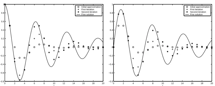
Figure 1. First few iterations of the original parareal algorithm for the model

problemu00_=−u.

we find for the n-th coefficientek

n of the functionρk the bound

ek

n≤γα

k_βn−k−1₍n

k+1) +δ(nn−1)(α+β)n−1.

We thus obtain

||Enk|| ≤C

k+2_(∆tp+1_{+ ∆T}p+1₎k+1_{(1 +C}

2∆T)n−k−1(nk+1)

+C∆tp+1n(1 +C2∆T)n−1

≤C1 T

k+1

n

(k+ 1)!e

C2(Tn−Tk+1)_∆Tp(k+1)_+C

3TneC2Tn∆tp,

(5.12)

which proves the theorem.

Remark 5.4. From Theorem 5.3 we see that at each iteration the accuracy of the method improves,

but it is limited by the accuracy of the method given by the fine propagatorF. More precisely,

the error is bounded by

||Enk|| ≤Ckmax(∆T(k+1)p,∆tp).

6.

_{Numerical Experiments}

We first consider the simple model problem u00 _{= −u with initial conditions u(0) = 1 and}

u0_{(0) = 0. We transform the equation into a first order system with two components, and perform}

the simulations on the time interval [0,20]. We choose for the coarse time step ∆T = 1, and for

the fine time step ∆t= 1/6. In Figure 1, we show the first few iterations of the original parareal

0 2 4 6 8 10 12 14 16 18 20 −0.8 −0.6 −0.4 −0.2 0 0.2 0.4 0.6 0.8 1 t Initial approximation First iteration Fine solution

0 2 4 6 8 10 12 14 16 18 20

−0.8 −0.6 −0.4 −0.2 0 0.2 0.4 0.6 0.8 1 t Initial approximation First iteration Fine solution

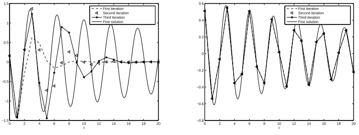
Figure 2. Initial approximation and first iteration of the modified parareal

algo-rithm for the model problemu00_=−u.

0 2 4 6 8 10 12 14 16 18 20 −1.5 −1 −0.5 0 0.5 1 1.5 t First iteration Second iteration Third iteration Fine solution

0 2 4 6 8 10 12 14 16 18 20 −0.8 −0.6 −0.4 −0.2 0 0.2 0.4 0.6 t First iteration Second iteration Third iteration Fine solution

Figure 3. The first component of the solution for u00₊Ku _{= 0 after the first few} iterations of the original parareal algorithm and of the modified algorithm.

In Figure 3, we consider the model problemu00_{+Ku= 0 withKa random matrix of dimension}

100, for the time interval [0,20]. We compare the first component of the solution obtained with the

classical parareal algorithm and with the modified algorithm. We notice again that the classical parareal algorithm converges slowly, and the convergence is better for short time than for long time. In contrast, the modified parareal algorithm converges very rapidly.

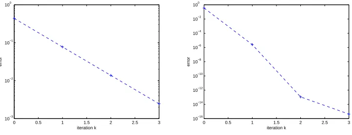
In Figure 4, we show the error between the solutions of this system on the time interval [0,5],

obtained with the fine propagator and the parareal method, using first the original parareal algo-rithm and then the modified one, for the first three iterations. We can see that the convergence is significantly improved using the modified parareal algorithm.

We finally show a comparison for the case of the heat equationut−uxx= 0 with homogeneous

Dirichlet conditions on the spatial domain [0,1], and with a random initial condition. The

time-interval is [0,1]. The modified parareal algorithm also converges faster, as one can see in Figure 5,

where we plotted the error measured in the L∞_{(0, T, L}2_{)-norm between the fine solution and the}

0 0.5 1 1.5 2 2.5 3 100.1

100.3 100.5 100.7

100.9

iteration k

error

0 0.5 1 1.5 2 2.5 3

10−14 10−12 10−10 10−8 10−6 10−4 10−2 100 102

iteration k

error

Figure 4. Error for the classical and the modified parareal algorithm foru00₊Ku_{= 0.}

0 0.5 1 1.5 2 2.5 3

10−3

10−2 10−1

100

iteration k

error

0 0.5 1 1.5 2 2.5 3

10−16

10−14

10−12

10−10

10−8

10−6

10−4

10−2

100

iteration k

error

Figure 5. Error for the classical and the modified parareal algorithm, applied to the heat equation.

References

[1] G. Bal,On the convergence and the stability of the parareal algorithm to solve partial differential equations, Domain decomposition methods in science and engineering, Lect. Notes Comput. Sci. Eng., 40, Springer-Verlag (2004), pp. 425–432.

[2] C. Farhat and M. Chandesris,Time-decomposed parallel time-integrators: theory and feasibility studies for fluid, structure, and fluid-structure applications, Internat. J. Numer. Methods Engrg., 58 (2003), pp. 1397–1434. [3] C. Farhat, J. Cortial, C. Dastillung, and H. Bavestrello,Time-parallel implicit integrators for the near-real-time prediction of linear structural dynamic responses, Internat. J. Numer. Methods Engrg., 67 (2006), pp. 697–724.

[4] M. J. Gander and E. Hairer,Nonlinear convergence analysis for the parareal algorithm. Lect. Notes Comput. Sci. Eng., 60, Springer-Verlag (2007), pp. 45–56.

[5] M. J. Gander and S. Vanderwalle,Analysis of the parareal time-parallel time-integration method, SIAM J. Sci. Comput. 29(2) (2007), pp. 556–578.

[6] J.-L. Lions, Y. Maday, and G. Turinici,R´esolution d’EDP par un sch´ema en temps “parar´eel”, C. R. Acad. Sci. Paris S´er. I Math., 332 (2001), pp. 661–668.