Gabriel Caloz & Monique Dauge, Editors
MULTILEVEL GRADIENT-BASED METHODS IN AERODYNAMIC SHAPE
DESIGN
Massimiliano Martinelli
1and Francois Beux
1Abstract. A gradient-based method coupled with a multilevel approach is proposed for shape design in aerodynamics. This method extends an existing multilevel gradient-based formulation to another type of control subspaces, i.e. considering another set of subparametrisations and prolongation op-erators. More precisely, B´ezier control points associated with the property of degree elevation are involved instead of shape grid-points coordinates and polynomial interpolation. The good behaviour of the new formulation is demonstrated on a classical 2D nozzle inverse problem considering an adjoint formulation as well as an approximate gradient associated to a one-shot method.
R´esum´e. Une m´ethode de type gradient associ´ee `a une approche multiniveau est propos´ee dans le cadre de probl`emes d’optimisation de forme en a´erodynamique. Cette m´ethode g´en´eralise une formulation d´ej`a existante de m´ethode de gradient multiniveau consid´erant un autre type de sous-espace de contrˆole, c’est `a dire consid´erant un autre ensemble de sous-param´etrisation et d’op´erateur de prolongement. Plus pr´ecisement, des points de contrˆole de B´ezier associ´es `a la propri´et´e d’´el´evation de degr´e sont utilis´es au lieu des coordonn´ees des points du maillage sur la fronti`ere et une interpolation polynomiale. Le bon comportement de la nouvelle formulation est illustr´e pour le cas d’un probl`eme inverse classique d’une tuy`ere bidimensionelle consid´erant aussi bien une m´ethode de l’adjoint que le calcul d’un gradient approch´e associ´e `a une m´ethode de type “one-shot”.
Introduction
In this study, we are interested in gradient-like methods for shape optimisation problems in aerodynamics. More particularly, we consider the computation of a discrete gradient, i.e. the differentiation is performed after a complete discretisation of the governing equations. In this context, a natural choice of parametrisation is to consider the coordinates of the grid-points localised on the shape which should be optimised. Indeed, this kind of parametrisation allows a direct correlation with the explicit representation of the shape in the discrete cost functional. Nevertheless, in this case, non-smooth profiles can appear during the shape optimisation process. This phenomenon, particularly critical for shape grid-points parametrisation, can be also linked with a regularity loss of the gradient with respect to the control variables, already verified in the continuous case (see, e.g. [3] or [6]). Thus, to avoid high frequencies in the discrete gradient involved in the shape updating, a preconditioning procedure should be applied. The necessity to define a smoothing operator can be also understood through the consistent approximation theory proposed by Polak (see [7]). A possible way to precondition is based on the inversion of a Laplace-Beltrami operator, which corresponds to a change of metric on which the minimisation is done [6, 8]. Alternatively, in [3], an adequate gain of regularity for the gradient is obtained through the use of an additive multilevel approach. Note that multilevel concepts, in the context of gradient-like methods
1Scuola Normale Superiore di Pisa, Piazza dei Cavalieri, 7 - 56126 Pisa (Italy); e-mail:[email protected] & [email protected] c
EDP Sciences, SMAI 2007
for optimum shape design, have been initially ideated in [2]. In this approach, the minimisation is done alternatively on different subsets of control parameters according to multigrid-like cycles of multiplicative type. More particularly, using shape grid-point coordinates as design variables, a hierarchical parametrisation was defined considering different subsets of parameters extracted from the complete parameterisation, which can be prolongated to the higher level by linear mapping. This approach has been also defined to make the convergence rate of a gradient-based method almost independent of the number of control parameters.
Alternatively to shape grid-points, a polynomial representation of the shape is often used allowing a more compact description with only few control parameters. In particular, in [4], a multilevel approach is proposed considering as control parameters a set of B´ezier control points. Nevertheless, this approach sensibly differs from the method defined in [2] since, in particular, the study was not focused on gradient-based methods.
In the present study, a new multilevel strategy based on the use of B´ezier control points, but in the context of a gradient-based method, is proposed. Indeed, the present algorithm is grounded on some basic concepts yet proposed in [4], as, for instance, the degree elevation property of the B´ezier curves, but on another hand, can be interpreted as a multilevel strategy as defined in [2], in which a particular prolongation operator is applied.
A first validation is proposed on a classical 2D nozzle inverse problem for inviscid flows.
1.
Gradient-based method and multilevel approach
The multilevel method, proposed in [2], is based on a change of control space. More precisely, letEandF be two Hilbert spaces and P :F −→E linear, instead of a direct minimisation of the functionalj in the spaceE
of the control variables, the gradient algorithm is applied for the minimisation ofj◦P inF. Furthermore, the resulting algorithm remains a descent method in the spaceE. In the context of a discrete gradient computation in aerodynamic shape design, a practical example can be to consider as control variables the ordinates of the
mshape grid-points, i.e. takeE=Rm.
Different spacesF are then considered, each of them corresponding to a subset of points extracted from the complete parametrisation. For each levell, a linear applicationP(l):F =Rnl−→E=Rm is defined allowing to prolonged the nl parameters on the finest level. Then, at iteration r and level l, the control variables are updated as follows:
γr+1=γr−ωrP(l)(P(l))∗gr with ωr∈Randgr∈Rm, (1)
gr being the gradient of the cost functional at iteration r, and, (P(l))∗ the adjoint
P(l) adjoint, which is associated to the transpose of the matrix M(l) ∈ Rm×nl relative toP(l). Note that, only the differentiation of the cost functional with respect to the complete parametrisation is needed since the minimisation on the coarser levels appears uniquely through the matrix M(l)(M(l))T ∈
Rm×m. Thus, this algorithm can be also interpreted as a preconditioned gradient method. On another hand, the level choice at each optimisation iteration is determinate by a strategy of level changes similar to multilevel/multigrid strategies used for the resolution of partial differential equations (as, for instance, V-cycles). The particular algorithm is then totally definite by the choice of the operatorP(l). For shape-grid points as control parameters, a natural way to define the prolongation operator is to use interpolations. Different interpolations have been considered in [2] giving convergence curves sensibly different. Finally, a Hermitian cubic interpolation coupled with a set of embedded subparametrisations (for each increase of level, the number of points is doubled), has been chosen in [2], and, also used in successive works (see, e.g. [5]).
follows:
fori= 1,· · ·, m γr+1i= γri−ωr nl
X
k=1
M(l)ik 1 ǫ
j
γr+ǫP(l)(ek)
−j(γr)
(2)
in whichek is thek-th element of the canonical basis ofRnl,ǫan adequate small given parameter.
Furthermore, in [5], this multilevel/divided-differences formulation has been also used in a one-shot approach [9] in which the flow equations are progressively solved. In practical, at each optimisation iteration, the flow evaluations are done considering only a very partial resolution of the steady governing equations (only few pseudo-time steps using in the pseudo-unsteady approach and few iterations of the iterative method for solving the linear system involved in the implicit linearised scheme).
2.
Multilevel method associated to B´
ezier parametrisation
A B´ezier curve of degreencan be defined according to its parametrisation, i.e.:
S(t) = (x(t), y(t)) =
n
X
q=0
Bnq(t)Sq with t∈[0,1] (3)
whereSq= (xq, yq) is theq-th B´ezier control point whileBq
n(t) corresponds to theq-th Bernstein polynomial.
The ordinates of the shape grid-points, i.e. γ= (y0Γ,· · ·, ymΓ)T, are here considered as design variables.
Further-more, the parameters (tk)k=0,m being given (t0= 0< t1<· · ·< tm= 1) and using relation (3) withy(tk) =ykΓ
fork= 0,· · ·, m, it clearly appears that each control variable can be expressed as a linear combination of the ordinates of the B´ezier control points α= (y0,· · · , yn)T. Thus, the following linear operator from αto γ can be considered:
P : Rn+1 −→ Rm+1
α 7−→ γ=P(α) =M α where Mij =Bj n(ti).
Then, thanks to the linearity ofP, it is possible to define a strategy similar to the original multilevel approach [2], where instead of a subset of boundary grid-points, each subparametrisation is a set of B´ezier control points. In this case, the following algorithm can be defined:
γr+1=γr−ωrd(rl)with ωr∈Randγr, γr+1 andd(rl)∈Rm+1
in which the descent direction at iterationrand levell is defined by:
k= 0,· · ·, m
d(rl)
k
=
m
X
j=0
nl
X
q=0 Bnql(t
(l) k )B
q nl(t
(l) j )
| {z }
M(l)(M(l))T kj
(gr)j (4)
Nevertheless, the definition of the subparametrisations is, here, not so obvious. Indeed, the abscissae of shape grid-points ({xΓk}k=0,m) being given, at each level, X(l) = (x(
l) 0 ,· · ·, x
(l)
nl)T with nl > nl−1 and T(l) = (t(0l),· · ·, t
(l)
m)T should be defined such that (3) be always verified, i.e.:
xΓk =x(t (l) k ) =
nl
X
q=0
Bnlq (t(kl))xq(l) for k= 0,· · ·, m (5)
Let us now suppose that the parametrisation on the coarsest level has been yet defined with X(0) andT(0)
0 1000 2000 3000 4000 5000 6000 7000 8000 9000 10000 −8
−7 −6 −5 −4 −3 −2 −1 0 1
Pseudo−time iterations
Log( Functional )
Bezier 15−10−5 Shape pts. 15−7−3 Bezier 15 Shape pts. 15
0 1000 2000 3000 4000 5000 6000 7000 8000 9000 10000 −5
−4 −3 −2 −1 0 1 2
Pseudo−time iterations
Log( ||descent direction|| )
Bezier 15−10−5 Shape pts. 15−7−3 Bezier 15 Shape pts. 15
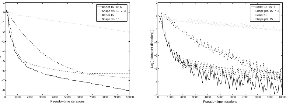
Figure 1. Convergence histories for j(γr) (left) and d(rl) (right) in the case of an adjoint gradient computation: comparison between shape grid-points and B´ezier parametrisations for both on one level (15 parameters) and a V-cycle multilevel approach on three levels.
simply choosing an uniform distribution for both X(0) and T(0). In order to define a parametrisation on the other levels, the property of degree elevation of the B´ezier curves is used here. Indeed, the degree-elevation property allows to increase the degree and the number of control points of a B´ezier curve without any change on the distribution of the parameterst(see, e.g. [4]). Then, the parameters {tk}k=0,m keep unchanged on all the
levels, i.e. t(kl)=t (0)
k ≡tk fork= 0,· · ·, met l >0, whileX(
l) forl >0 is obtained applying successively the
degree-elevation algorithm until obtainingnl+ 1 abscissae. More precisely, the following algorithm is considered to obtainX(l)from X(0) (with the conventionx−
1= 0):
s←−1
Forq= 0,· · · , n0 xq ←−x(0)q
Repeat untils=l
ObtainX(s) fromX(s−1) as follows: n←−ns−1
Repeat untiln=ns
xq←− q
n+ 1xq−1+
1− q n+ 1
xq for q= 0,· · ·, n+ 1
n←−n+ 1
s←−s+ 1
X(l)←−(x
0,· · ·, xn)T
3.
A numerical example: a 2D nozzle inverse problem
Let us consider a classical test-case already used for the multilevel approach associated to shape grid-point coordinates parametrisation [2, 5]. It is a 2D convergent-divergent nozzle inverse problem for inviscid subsonic flows (the flow is modelled, here, by the Euler equations). The corresponding cost functional is expressed as a boundary integral which involves the flow variables through the pressure field. An initial constant-section nozzle and a target sine shape are considered while the computational mesh is composed, here, of 423 nodes with 31 points on the upper boundary of the throat nozzle, i.e. where the shape should be optimised.
0 50 100 150 200 250 300 350 400 −9
−8 −7 −6 −5 −4 −3 −2 −1 0 1
Equiv. flow evaluations
Log( Functional )
Bezier 15−10−5 exact gradient Bezier 15−10−5 oneshot Shape pts. 15−7−3 exact gradient Shape pts. 15−7−3 oneshot
0 50 100 150 200 250 300 350 400 −6
−5 −4 −3 −2 −1 0 1
Equiv. flow evaluations
Log(||descent direction||)
Bezier 15−10−5 exact gradient Bezier 15−10−5 oneshot Shape pts. 15−7−3 exact gradient Shape pts. 15−7−3 oneshot
Figure 2. Convergence histories for j(γr) (left) and d(rl) (right): comparison between exact adjoint gradient computation and gradient approximate by divided differences associated with a one-shot approach.
0 0.2 0.4 0.6 0.8 1 1.2 1.4 1.6 1.8 2 0.15
0.2 0.25 0.3 0.35 0.4 0.45 0.5 0.55 0.6 0.65
Iter. 1 Iter. 5 Iter. 13 Iter. 25 Target
0 0.2 0.4 0.6 0.8 1 1.2 1.4 1.6 1.8 2 0.15
0.2 0.25 0.3 0.35 0.4 0.45 0.5 0.55 0.6 0.65
Iter. 1 Iter. 5 Iter. 13 Iter. 25 Target
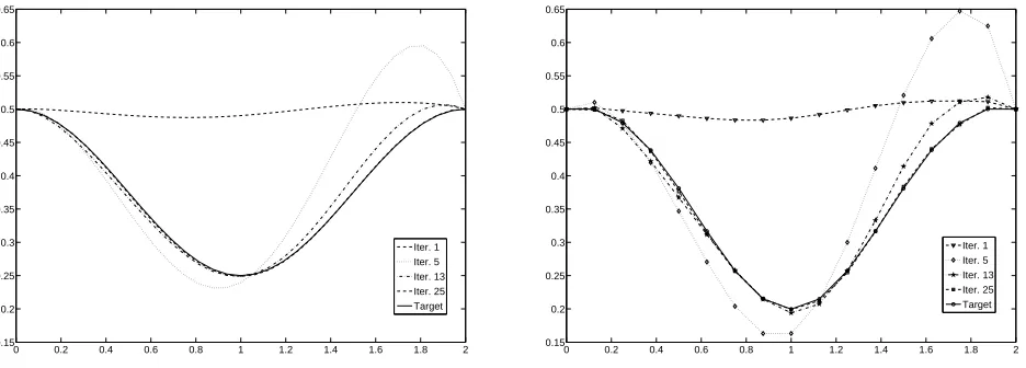
Figure 3. One-shot/multilevel approach using B´ezier parametrisation: successive shapes (left) and B´ezier control points (right). Comparison between the target solution and solutions after 1, 2, 4 and 7 V-cycles (i.e., after 1, 5, 13 and 25 optimisation iterations).
Nevertheless, it does not correspond to the same level of shape description since the B´ezier control points allow a more compact representation than the shape grid-points.
Fig. 2 reports the same V-cycle three-levels approaches applied both for the adjoint method and the divided-differences one associated with a one-shot approach. The good behaviour of the one-shot approach without adjoint, already obtained in [5], is also confirmed for the subparametrisation based on B´ezier curves. Moreover, the same improvement obtained by using the B´ezier parametrisation instead of the shape grid-points is observed with the multilevel/divided-differences one-shot approach. Fig. 3 shows the shape evolution during the optimi-sation process for the one-shot method with the B´ezier parametrioptimi-sation and the multilevel/divided-differences formulation. Note that, the cost for obtaining a converged flow solution corresponds approximatively to two V-cycles on three levels (5, 10 and 15 parameters) with the one-shot approach (i.e., here only one pseudo-time iteration and three iterations of the iterative method for solving the linear system). Thus, with a computational cost equivalent to four flow evaluations, we already obtain a shape very close to the target one. Fig. 3 also shows on the right frame, the evolution of the B´ezier control points. In this simple case, even if we consider an uniform distribution of the abscissae, the resulting distribution of the ordinates of the B´ezier control points is very regular without any oscillation. Thus, an adaptation of the parametrisation as proposed in [1] is not needful, here, at least in this particular case.
4.
Conclusion
In the present study, a multilevel gradient-based method for optimum shape design in aerodynamics is described. This approach starts from an existing formulation [2] based on an embedded parametrisation of shape grid-points and on interpolation operators. A new set of subparametrisations is then proposed, in which a coarse level is described by using B´ezier control points while the prolongation operator is obtained through the application of the degree elevation formula. Thus, this approach seems not so far from the one proposed in [4]. Nevertheless, contrary to [4], a descent direction method is always considered, and moreover, the control variables on the finest level are still the ordinates of the shape grid-points. Some numerical experiments have been done on a simple 2D nozzle inverse problem showing that the introduction of this new family of subparametrisations has suitable effects on the convergence behaviour. This is true considering an adjoint formulation as well as an approximate gradient associated to a one-shot method. Note that, since the B´ezier curves act as a basic tool for polynomial shape representation, one can also envisage to extend the formulation to more complex curves as B-splines, and also, to 3D case through, for instance, tensorial B´ezier parametrisation.
References
[1] B. Abou El Majd, J.-A. D´esid´eri and A. Janka, Nested and self-adaptive B´ezier parameterization for shape optimization,
International Conference on Control, Partial Differential Equations and Scientific Computing, Beijing, China, 13-16 Sept, 2004.
[2] F. Beux and A. Dervieux, A hierarchical approach for shape optimization,Engineering Computations,11/1, 25-48, 1994. [3] F. Courty and A. Dervieux, Multilevel functional Preconditioning for shape optimisation,International Journal of
Computa-tional Fluid Dynamics,20/7, 481-490, 2006.
[4] J.-A. D´esid´eri, Hierarchical optimum-shape algorithms using embedded B´ezier parameterizations, Numerical Methods for Scientific Computing, Variational Problems and Applications, E. Heikkola, Y. Kuznetsov, P. Neittaanm¨aki and O. Pironneau et aleds., CIMNE, chapter Hierarchical Optimum-Shape Algorithms Using Embedded B´ezier Parameterizations, 2003. [5] C. Held and A. Dervieux, One-shot airfoil optimisation without adjoint,Computers and Fluids,31/8, 1015-1049, 2002. [6] B. Mohammadi and O. Pironneau,Applied Shape Optimization for Fluids, Numerical Mathematics and Scientific Computation,
Oxford University press, 2001.
[7] E. Polak, Optimization: algorithms and consistent approximations,Applied Mathematical Sciences, 124, Springer-Verlag, New York, 1997.
[8] J. Reuther and A. Jameson, Aerodynamic shape optimization of wing and wing-body configurations using control theory, AIAA Paper, 95-0123, 1995.