Destabilization of Localized Structures in Reaction-Diffusion Systems Induced by Delayed Feedback

(1)

M. Belhaq, P. Lafitte and T. Leli`evre Editors

DESTABILIZATION OF LOCALIZED STRUCTURES IN REACTION-DIFFUSION

SYSTEMS INDUCED BY DELAYED FEEDBACK

Svetlana V. Gurevich

1

and Rudolf Friedrich

1

Abstract. We are interested in the stability of two-dimensional localized structures in reaction-diffusion systems subjected to a delayed feedback. We show that the presence of the delay can induce complex behavior of the localized structures, including, e.g., spontaneous motion or breathing of the localized objects. In the case of spontaneous motion, the corresponding order parameter equation for the position of the localized structure is derived. In addition, numerical simulations are carried out showing good agreement with the analytical predictions.

Introduction

In the field of nonlinear dynamics, control and engineering of dynamical behaviour of spatio-temporal patterns in high-dimensional nonequilibrium systems is one of the key issues of recent research [3, 13]. In particular, controlling of dissipative localized structures, single isolated, randomly distributed or organized in clusters have been of increasing interest in recent years. Self-organized localized solitary patterns in dissipative systems turned out to be of particular interest for fundamental research as well as for applications [14, 15, 17]. We refer to these objects as dissipative solitons (DSs), following Ref. [1, 14, 15, 17]. Nevertheless, other nomenclature can also be found in the literature, e.g., autosolitons [9], oscillons [10] as well as spots and pulses in neuroscience [2, 21] and different chemical systems [13].

In order to control such a complex phenomenon, different approaches have been proposed. In particular, the onset of pulse propagation in the FitzHugh-Nagumo (FHN) system with control by augmented transmission capability that is provided either along nonlocal spatial coupling or by time-delayed feedback was studied in [21]. Recently, the properties of 2D bright and dark dissipative structures in a real Swift-Hohenberg equation subjected to delayed feedback were investigated in [22, 23]. In particular, it was shown that when the product of the delay time and the feedback amplitude exceeds some critical value, single cavity solitons start to move in arbitrary direction. Moreover, in [7] the influence of the delayed feedback on the stability properties of single DS in real Swift-Hohenberg equation was investigated in details. Depending on delay time and delay strength coefficient, various destabilization scenarios were obtained, including breathing DSs as well as multi-mode oscillatory instabilities leading to complex spatio-temporal patterns.

1 _{Institut for Theoretical Physics, University of M¨}_{unster, Wilhelm-Klemm-Str. 9, 48149 M¨}_{unster, Germany,}

E-mail : [email protected]

c

EDP Sciences, SMAI 2013

(2)

In this paper we investigate the influence of the delayed feedback on the stabilty properties of single DS in the three-component reaction-diffusion (RD) system with one activator and two inhibitors :

∂tu=Du∆u+f(u)−κ3v−κ4w+κ1+α u(t)−u(t−τ) ,

η ∂tv=Dv∆v+u−v+η α v(t)−v(t−τ) ,

θ ∂tw=Dw∆w+u−w+θ α w(t)−w(t−τ) .

(1)

Here u = u(r, t) is the activating component, whereas v = v(r, t) and w = w(r, t) denote the inhibiting components and r ⊂ R2. In the polynomial nonlinear function f(u) = λu−u3 _{the coefficient} _λ _{is positive.} Du, Dv, Dw denote the (positive) diffusion coefficients of the components, whereas the positive parameters η and θ represent dimensionless constants, being the ratios of the characteristic times of both inhibitors with respect to the that of the activator. The coefficient κ1 violates the inversion symmetry (u 7→ −u) and has arbitrary sign. The constantsκ3andκ4 staying in reaction term are also positive, indicating inhibiting nature of v andw. Finally, τ denotes the delay time, whereas the positive parameterαis the delay rate. Notice that the delayed feedback term in Eq. (1) is a simple form of the famous Pyragas delayed feedback control [18, 19], which was successfully used to control unstable trajectories in diverse systems, e.g., [11, 12, 16].

In the absence of the delayed feedback the system (1) was first introduced in [20, 24] as an extension of the phenomenological model for a planar dc gas-discharge system with semiconductor electrode. On the other hand, the system (1) can be considerd as a three-component extension of the FHN system for nerve pulse transmission, which is widely used in various areas of research [2, 4, 8, 17].

In this paper we are interested in the stability properties of the single DS in the system (1). We shall show that delayed feedback can lead to different instabilities of the soliton, including spontaneous motion, spontaneous breathing as well as complex oscillatory behavior. We also show that, using the product of the delay time τ and delay rate α as a control paramenter, one can easily control the instability type. Moreover, in the case of spontaneous motion of the DS we derive the order parameter equation for the position of the soliton and determine the analytical expression for its velocity.

1. Linear stability analysis

We start from the general form of the evolution equation :

∂tq(r, t) =L₍_∇₎q(r, t) +αE q(r, t)−q(r, t−τ)

, (2)

where in our case q=q(x, t) = (u , v , w)T_{, is a vector-function,} _x_{= (x , y)} _∈_R2 _{and the operator} _L₍_∇_{) is a} nonlinear operator

L₌_D_∇2₊_R(_·_).

Here∇2 _{denotes the Laplace operator, the diagonal matrix}_D_{contains the diffusion constants of}_{u , v , w}_{on the} principal diagonal, vectorR(q) stands for nonlinear reaction term and E is an identity matrix.

Linear stability analysis for

α

= 0

Let q0(x) be a stationary solution of the system (2) with α = 0, i.e., Lq0 = 0. In the simplest case it is a

stationary localized structure with rotational symmetry. Linear stability of this solution can be analyzed by a substitution of the ansatzq(x, t) =q0(x) +w(x, t), wherew(x, t) =ϕ(x)eµ tin Eq. (2), resulting in the linear

eigenvalue problem

L′₍q0)ϕ=µϕ, (3)

where the linear operator L′₍q0) is the linearization of Laroundq0,µ is the set of eigenvalues ofL′(q0) and ϕ(x) are the corresponding eigenfunctions. As can be easily shown for the system (1) the operatorL′(q0) is not

Hermitian. This implies that the eigenvaluesµand corresponding eigenfunctions (or modes)ϕ(x) are in general

(3)

an eigenvalue of the operator L′₍q0), corresponding to two independent neutral eigenfunctions (one for each

spatial direction), which in the following will be called Goldstone, or neutral modes. They can be identified as the first derivatives ofq0 with respect to x, i.e., ϕGx =∂q0/∂x. In the case of RD systems one can speak

about a compact operator L′₍_q

0), namely the operator, whose continuous spectrum is separated from zero.

That is, only a finite number of modes, whose eigenvalues are close to zero and belong to the discrete spectrum, can become unstable by the change of some control parameter. These critical modes can be found using the ansatz : w∼wnei n φ. Then the influence of the modes with differentn on the radial-symmetrical DS q0 can

be understood as follows : the mode withn= 0 (the breathing mode [5]) results in the change of the size of the DS ; the mode withn= 1 describes the shift of the solution andn≥2 causes different deformations of the DS. Now let us assume that the real parts of all eigenvalues of (3) except for µ= 0 are negative.This implies the stationary solutionq0forα= 0 is stable.

Linear stability analysis for

α >

0

Since the stationary solutionq0(r) is time-independent, it remains a stationary solution of (2) for all values

of α. Since the operators L′₍q0) and E commute, linear stability of the solution for α >0 can be constructed

from the spectrum of L′₍q0) via the delayed eigenvalue problem

L′₍q0)ϕ=

λ−α 1−e−λ τ

ϕ, (4)

where the eigenvaluesλare determined as solutions of the transcendental equation

µ=λ−α 1−e−λ τ

. (5)

That is, the stationary solution q0 remains stable when real parts of λ(µ) <0 for all criticalµ belonging to

the spectrum of the operatorL′₍q0). Nevertheless, the stationary DS can loose its stability with the change of

some control parameter, e.g., the product of delay time τ and feedback rateα. Indeed, if we are interested in real solutions of Eq. (5), corresponding toµ= 0, two different solutionsλ1,2, corresponding to the neutral mode can be obtained [23] :

λ1= 0, λ2= 2 τ

(a−1)

a ,

wherea:=ατ. Hence, the neutral mode remains in the presence of delayed feedback. One can also see that λ2 remains negative for all valuesa <1. However, fora >1 these eigenvalue becomes positive, leading to the drift of the DS [7, 22]. It has to be noted that in general all solutions of transcendental equation (5) are complex. That is, ifµ=δ±iω, one can try to find the critical delay timeτc for the fixed value of the control parameter a, that the correspondingλcrosses the imaginary axis, i.e.,λ=±iβ. It can be shown that for the all real values

of µ, µ =δ < 0 the stationary solution of delayed problem remains stable for a ≤max

−δ/2τ ,1

[7]. For

complex values ofµthe corresponding condition is much more complicated and cannot be written in a compact form. However, one can find the critical delay timeτc by means of the solvability condition :

±arccos(1 +x) + 2πn−ωa δ x=±a

p

1−(1 +x)2_, _n_∈_Z_, ₍₆₎

where τc :=x a/δ. Note that for small values ofδ, nontrivial solutions β 6= 0 of the last equation are possible fora <1. Hence, oscillatory modes can become unstable before the induced drift sets in.

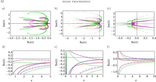
This statement becomes more clear if we solve Eq. (5) numerically for different values of µ, corresponding to discrete critical modes of the operator L′₍q0) and different values of the control parameter aand time delay τ

(see Fig. 1).

(4)

a) b) (c)

d) e) f)

Figure 1. Evolution behavior of the eigenvalues in the complex plane ( a)–c) ), corresponding to the first four critical eigenmodes induced by the change of the delay time τ as well as the real parts of these eigenvalues as a function ofτ is presented. a), d)a= 0.5 ; b), e)a= 0.8 ; c), f)a= 1.05. The eigenvalues corresponding to different eigenfunctions differ in colors.

and the corresponding solution is stable. If we increase the value ofa, e.g.,a= 0.8 (Fig. 1 b), e)) one can see, that eigenvalues corresponding to complexµbecome unstable for small values ofτ. However, with increasing of τ, all complex eigenvalues move back into the half-plane Re(λ)<0 and the stationary solution becomes stable. Notice that the critical delay time, for which each eigenvalue becomes stable, can be calculated by means of solvability condition (6). Finally, if the value of the control parameter exeeds one (see Fig. 1 c), f) ), all modes become unstable for small values of τ. For large values of τ, however, all complex eigenvalues become stable again, and only one type of instability, corresponding to the drift of DS remains. It has to be emphasized, that solvability condition (6) gives the possibility of the effective control of the instability type. However, one can also see (Fig. 1 e), f)) that in particular for small delay times different modes are unstable simultaneously, that is, the dynamical behavior in this region can be very complex.

2. Application to reaction-diffusion system

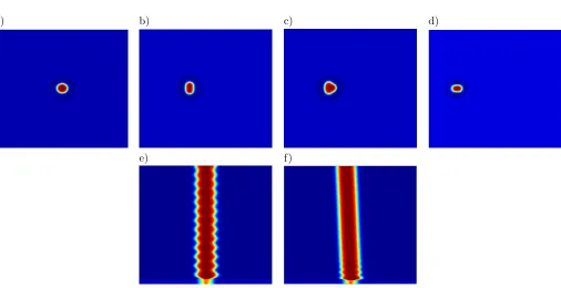
Such a complex behavior of DS is illustrated in Fig. (2), where the result of direct numerical simulation of Eq. (1) for a = 1.05 and different values of τ is presented. Numerical simulations have been performed on the two-dimensional square domain Ω = [−2,2]×[−2,2] with periodic boundary conditions using a pseudo-spectral method with 512×512 grid points, whereas a Runge-Kutta 4 scheme is employed for the time stepping. Figure 2 shows the time evolution of the activator for τ = 2.4. In this parameter range, several modes are unstable simultaneously : DS moves to the left with the constant velocity,n= 0 influences its size (Fig. 2 a)), whereas modes with n=±2 (Fig. 2 b), d)) andn= 3 (Fig. 2 c)) are responsible for different deformations of DS.

(5)

a) b) c) d)

e) f)

Figure 2. (a-d) Example of the motion and complex form-deformation of single DS obtained by numerical simulation of Eq. (1). Activator distributionu(x, y, t) for four different times is presented . a) t = 9 - the size of the solution increases ; b) t= 81, c) t= 96 and d) t = 147 shows the influence of the modes with n = 2, n = 3, and n = −2. (e-f) Space-time plots of the activator distribution for a = 1.05 and different values of τ obtained from numerical solution of Eq. (1). e)τ= 6.0, the solution oscillates with the constant amplitude ; f)τ= 8.0, after relaxation oscillations, DS moves to the left with the constant velocity. Parameters are : Du = 4.7·10−3_, _Dv _{= 0,} _Dw _{= 0.01,} _λ_{= 5.67,} _κ1 ₌ ₋_1.04, _κ3 _{= 1.0,} _κ4 _{= 3.33,} _η _{= 0.7,} θ = 0.01. The calculation was performed on the rectangular domain Ω = [−2,2]×[−2,2] with periodic boundary conditions using a pseudo-spectral method with 512×512 grid points, whereas a Runge-Kutta 4 scheme is employed for the time stepping.

the time dymanics is mostly governed by the mode n= 0, whereas in Figure 2 f) induced drift-bifurcation is demonstrated for τ = 8.0. One can also the influence of the stable modes on the dynamics of moving DS in form of relaxation oscillations for small simulation times.

3. _{Order parameter equation}

Now let us choose the control parametera >1 and let the time delayτ be relative large, that is, only induced drift instability determinates the time behavior of the system. The question we are interested is whether it would be possible to understand such an instability in terms of order parameter equation. To answer the question we perform the ansatz

q(x, t) =e−R(t)∇

q0(x) +w(x, t)

, (7)

where the operator e−R(t)∇5 _{generates a shift of the soliton located at}_x_{= 0 to the location}_R_{(t) and}_w₍_x_{, t)} is the deformation of the solution which is given by the sum of stable modes of the operator L′₍_q

0), i.e., w(x, t) =P

j ϕj(x)e

λjt.Our goal is to obtain an evolution equation for the position of the soliton as well as

(6)

the lowest order proportional to (Rt−Rt−τ)2, i.e.,w= (Rt−Rt−τ)2X with unknown functionX and is given

by [7]

∂w

∂t =L

′₍_q

0)w+α(wt−wt−τ)−

α 2

Rt−Rt−τ

∇ 2

q0. (8)

As was mentioned above we suppose that all critical modes except for the neutral ones are stable. We look for stationary states of the shape deformation. This yields

∂w

∂t = 0, w(x, t)≃w(x, t−τ) (9)

and the unknown functionX can be found by means of the following equation :

L′₍q0)X =

α

2∇∇q0. (10)

That is, we can calculate the shape deformation by inversion of the linear operatorL′₍_q 0).

An equation for the positionR(t) can be obtained by requiring that the shape deformation is orthogonal to the corresponding neutral modeϕG†x of the adjoint operatorL

′_†

(q0) resulting in an equation

˙

R = α Rt−Rt−τ

−α

6

h∇ϕG†x |∇ϕGxi

hϕG†x |ϕGxi

Rt−Rt−τ 2

Rt−Rt−τ

−hϕ G†

x |(∇wt− ∇wt−τ)i hϕG†x |ϕGxi

.

Because of the assumption on stationary shape deformations (9), the last term disappears and the delayed differential equation for the shift of the localized structure is obtained :

˙

R=α Rt−Rt−τ

−α

6

h∇ϕG†x |∇ϕGxi

hϕG†x |ϕGxi

Rt−Rt−τ 2

Rt−Rt−τ

. (11)

Notice that because of the assumption (9), the delay-induced drift bifurcation of the single DS takes place to the lowest order without change of shape. This makes such an instability behavior different from the classical drift-bifurcation [6].

In order to calculate analytically the velocitycof the soliton near the bifurcation pointa= 1, i.e., fora= 1 +ε, ε≪1 we make the ansatzRt=x+c t. Substituting this relation into Eq. (11) we obtain

c=±1 τ

s 6ε

β(1 +ǫ), (12)

with the constant factor β :=h∇ϕG†

x |∇ϕGxi/hϕG†x |ϕGxi. One can see that the velocity is a function of the delay

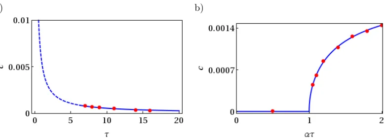
time τ as well as the distance to the bifurcation point ε. In order to compare this prediction with a direct numerical simulation, we first calculate the velocityc given by Eq. (12) and that of the single DS obtained by a 2D numerical simulation. This is presented in Fig. 3. One can see that the agreement is good even for rather large values ofaandε.

4. Conclusion

(7)

a) b)

Figure 3. Velocity of a single moving DS by means of Eq. (12) as a function of a) delay time τ for fixeda = 1.05 ; b) control parametera for fixed τ = 14.0 The red circles indicate the corresponding velocity obtained by direct numerical simulations. Dashed line indicates the control parameter range where other modes are also unstable.

References

[1] C.I. Christov and M.G. Velarde. Dissipative solitons.Physica D : Nonlinear Phenomena, 86(1-2) :323 – 347, 1995.

[2] Markus A. Dahlem, Rudolf Graf, Anthony J. Strong, Jens P. Dreier, Yuliya A. Dahlem, Michaela Sieber, Wolfgang Hanke, Klaus Podoll, and Eckehard Sch¨oll. Two-dimensional wave patterns of spreading depolarization : Retracting, re-entrant, and stationary waves.Physica D : Nonlinear Phenomena, 239(11) :889 – 903, 2010.

[3] H. G. Schuster E. Sch¨oll, editor.Handbook of Chaos Control. Wiley-VCH Verlag GmbH & Co. KGaA, 2008.

[4] H. Engel, F.-J. Niedernostheide, H.-G. Purwins, and E. Sch¨oll.Self-Organization in Activator-Inhibitor-Systems : Semicon-ductors, Gas-Discharge and Chemical Active Media. Wissenschaft und Technik Verlag, Berlin, 1996.

[5] S. V. Gurevich, Sh. Amiranashvili, and H.-G. Purwins. Breathing dissipative solitons in three-component reaction-diffusion system.Physical Review E, 74 :066201, 2006.

[6] S. V. Gurevich, H. U. B¨odeker, A. S. Moskalenko, A. W. Liehr, and H.-G. Purwins. Drift bifurcation of dissipative solitons due to a change of shape : Experiment and theory.Physica D, 199(1-2) :115–128, 2004.

[7] S. V. Gurevich and R. Friedrich. Instabilities of localized structures in dissipative systems with delayed feedbacksubmitted to Phys. Rev. Lett., 2012

[8] R. Kapral and K. Showalter, editors.Chemical Waves and Patterns, volume 10 ofUnderstanding Chemical Reactivity. Kluwer Academic Publishers, Dordrecht, 1995.

[9] B. S. Kerner and V. V. Osipov.Autosolitons. A New Approach to Problems of Self-Organization and Turbulence, volume 61 ofFundamental Theories of Physics. Kluwer Academic Publishers, Dordrecht, 1994.

[10] O. Lioubashevski, Y. Hamiel, A. Agnon, Z. Reches, and J. Fineberg. Oscillons and propagating solitary waves in a vertically vibrated colloidal suspension.Physical Review Letters, 83(16) :3190–3, 1999.

[11] O. L¨uthje, S. Wolff, and G. Pfister. Control of chaotic taylor-couette flow with time-delayed feedback. Phys. Rev. Lett., 86 :1745–1748, Feb 2001.

[12] T Mausbach, T Klinger, and A Piel. Chaos and chaos control in a strongly driven thermionic plasma diode.PHYSICS OF PLASMAS, 6(10) :3817–3823, OCT 1999.

[13] Alexander S. Mikhailov and Kenneth Showalter. Control of waves, patterns and turbulence in chemical systems. Physics Reports, 425(2-3) :79 – 194, 2006.

[14] A. Ankiewicz N. Akhmediev, editor.Dissipative Solitons : From Optics to Biology and Medicine, volume 751 ofLecture Notes in Physics. Springer, Berlin.

[15] A. Ankiewicz N. Akhmediev, editor.Dissipative Solitons, volume 661 ofLecture Notes in Physics. Springer, Berlin, 2005. [16] Th. Pierre, G. Bonhomme, and A. Atipo. Controlling the chaotic regime of nonlinear ionization waves using the time-delay

autosynchronization method.Phys. Rev. Lett., 76 :2290–2293, Mar 1996.

[17] H.-G. Purwins, H.U. B¨odeker, and Sh. Amiranashvili. Dissipative solitons.Advances in Physics, 59(5) :485–701, 2010. [18] K. Pyragas and A. Tamaˇseviˇcius. Experimental control of chaos by delayed self-controlling feedback.Physics Letters A,

180(1-2) :99 – 102, 1993.

(8)

[20] C. P. Schenk, M. Or-Guil, M. Bode, and H.-G. Purwins. Interacting pulses in three-component reaction diffusion systems on two-dimensional domains.Physical Review Letters, 78 :3781–3784, 1997.

[21] Sch¨oll E. Dahlem M.A. Schneider, F.M. Controlling the onset of traveling pulses in excitable media by nonlocal spatial coupling and time-delayed feedback.Chaos, 19(1), 2009. cited By (since 1996) 8.

[22] M. Tlidi, A. G. Vladimirov, D. Pieroux, and D. Turaev. Spontaneous motion of cavity solitons induced by a delayed feedback. Phys. Rev. Lett., 103 :103904, Sep 2009.

[23] Tlidi, M., Vladimirov, A. G., Turaev, D., Kozyreff, G., Pieroux, D., and Erneux, T. Spontaneous motion of localized structures and localized patterns induced by delayed feedback.Eur. Phys. J. D, 59(1) :59–65, 2010.