SMAI Groupe MAS – Journ´ees MAS 2012 – Prix Neveu
DISSECTING THE CIRCLE, AT RANDOM
∗Nicolas Curien
1Abstract. Random laminations of the disk are the continuous limits of random non-crossing configurations of regular polygons. We provide an expository account on this subject. Initiated by the work of Aldous on the Brownian triangulation, this field now possesses many characters such as the random recursive triangulation, the stable laminations and the Markovian hyperbolic triangulation of the disk. We will review the properties and constructions of these objects as well as the close relationships they enjoy with the theory of continuous random trees. Some open questions are scattered along the text.
Introduction
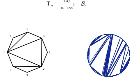
Let us begin our journey with the Brownian triangulation of Aldous. In the remaining of these pages, Pn denotes the regular polygon inscribed in the unit diskD:={z∈C:|z| ≤1} whose vertices are the
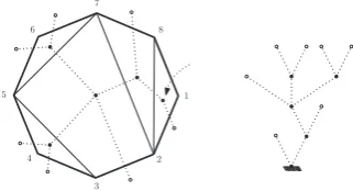
nth roots of unit. AtriangulationofPn is a subset of non-crossing (except at their endpoints) diagonals
that triangulatesPn, see Fig. 1. These triangulations are counted by Catalan numbers and are connected
to various combinatorial structures, see [22] for a beautiful application to the rotation distance problem. We are interested here inrandomtriangulations. Forn≥3we denote byTn a uniform triangulation of
Pn. Combinatorial properties ofTnhave been investigated in length [4, 12, 15]. From a geometrical point
of view, the random variableTn can also be seen as a random closed subset ofDand one can investigate
its limit geometry asn→ ∞. This has been proposed by David Aldous who proved the following:
Theorem (Aldous [2, 3]) We have the following convergence in distribution in the sense of Hausdorff distance on the closed subsets ofD
Tn (d) −−−−→
n→∞ B.
1
2 3 4 5
6 7
8
1
2 3 4 5
6 7
8
1
2 3 4 5
6 7
8
Figure 1. A triangulation of the octogon and a sample ofB.
∗Variation on Aldous’ original title : “Triangulating the circle, at random”.
1 CNRS et Universit´e Paris 6. LPMA, 4 place Jussieu 75005 Paris. E-mail: [email protected]
c
EDP Sciences, SMAI 2013
The random closed subsetBis calledthe Brownian triangulation of the disk. It is indeed a continuous triangulation since the complement ofBinsideDis made of countably many disjoint Euclidean triangles
a.s., see Fig. 1. This fractal object (it almost surely has Hausdorff dimension 3/2) has a fascinating structure and is connected to the Brownian continuum random tree [1] which can be thought of as its dual. The work of Aldous opened the doors for understanding the geometric structure of a large variety of random non-crossing structures yielding to a number of new objects such as the stable laminations ( [17] and Section 1.2), the recursive triangulation ( [10] and Section 2) or the Markovian hyperbolic triangulation ( [11] and Section 4).
Our goal is to present these nice objects and to convince the reader that the framework adopted here could provide a way to investigate continuous limits of discrete random trees.
Disclaimer : This is an expository work which is not meant to be fully rigorous nor exhaustive. The complete proofs as well as precise definitions of the objects considered can be found in the references. May the reader forgive our wordy and sketchy style.
Acknowledgments: We thank Igor Kortchemski for comments on a first version of this note. Thanks also go to the anonymous referee for a careful reading.
1.
The Brownian triangulation
In this section we give an overview of the construction of the Brownian triangulation B. The tools introduced for this purpose are of great use throughout the paper. Let us begin with a precise definition of non-crossing configurations of regular polygons.
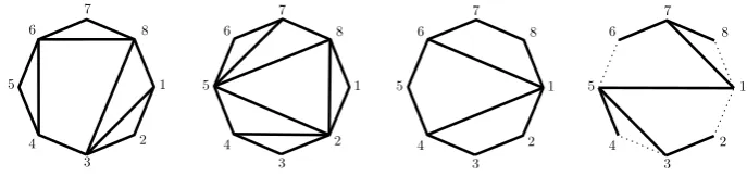
A non-crossing configuration (n.c.c. for short) of Pn is a subset of diagonals (and edges) of Pn that
are not crossing except at their endpoints. They are many classes of non-crossing configurations (see e.g. [14]), let us list a few:
• A triangulation is a n.c.c. that triangulates Pn, and more-generally for p ≥ 3 we speak of p
-angulation (quadrangulation, pentagulation, ...) when all the faces of the configuration (except the external face) havepadjacent edges,
• Adissection is a n.c.c. formed by the edges ofPn and some non-crossing diagonals, • Anon-crossing tree is a n.c.c. that is also a spanning tree of the vertices of Pn.
1
2 3 4 5
6 7
8
1
2 3 4 5
6 7
8
1
2 3 4 5
6 7
8
1
2 3 4 5
6 7
8
Figure 2. Examples of non-crossing configurations : from left to right, a dissection, a trian-gulation, a quadrangulation and a non-crossing tree of the octogon.
The general goal in these pages is to understand the geometric structure of random non-crossing config-urations asn→ ∞. To do so, it is convenient to see a n.c.c. as a closed subset of the unit disk (we shall always do so) and to ask for a limit theorem in the sense of the Hausdorff metric on closed subsets ofD.
We remind the reader that the Hausdorff distancedH between two closed subsetsA, B ⊂Dis the least
ε >0 such thatAis contained in theε-enlargement ofB and vice-versa. Recall also that
the set of closed subsets ofDiscompact fordH.
Theorem 1 ( [17] and [9]). If Cn is a uniform n.c.c. chosen in the class of p-angulations1 or dissections
or non-crossing trees ofPn then we have the convergence fordH
Cn (d) −−−−→
n→∞ B.
The combinatorial details of the class of n.c.c. considered thus vanish as n→ ∞and give rise to the Brownian triangulation. This limit result can be used to compute asymptotic quantities on n.c.c. For example the law of the arc (normalized by1/2π) intercepted by the longest diagonal in a random uniform
{p-angulation or dissection or non-crossing tree}ofPnconverges asn → ∞towards that of the Brownian
triangulation which is given [3, 12] by
1
π
3x−1
x2(1−x)2√1−2x113≤x≤ 1 2dx.
We let the reader think about many other applications of Theorem 1.
Laminations and continuous triangulations. Using terminology of geometers, we call a geodesic
lamination of the disk (lamination for short) any closed subset of the unit diskDthat can be written as
a disjoint union of diagonals[eix, eiy]forx, y∈
Rthat are not intersecting insideD, see [6]. In particular,
any n.c.c. of Pn can be seen as a finite lamination. It is fairly easy to see that the set of laminations is
closed for dH. A continuous triangulation is a lamination whose complement in D is made of disjoint
open Euclidean triangles. Equivalently, they consist of the laminations that are maximal for the inclusion relation, see [6, 20].
Using this vocabulary, the Brownian triangulation is indeed a continuous triangulation (and a lamina-tion) almost surely. This fact could seem obvious when B is considered as the limit of uniform discrete triangulations of Pn but less clear when considered as the limit of uniform quadrangulations! As all
characters of the Brownian family, the Brownian triangulation is a fractal object. Indeed, almost surely, no distinct triangles of D\B share an edge and it is shown in [20] (and sketched in [3]) that
dim(B) = 3
2, a.s. (1)
Without giving a proof of Theorem 1, let us introduce the main techniques and ideas it contains. For sake of simplicity we stick to the case of discrete triangulations.
1.1.
Duality and contour function
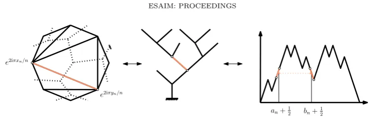
There is an obvious (once remarked) duality between triangulations ofPn and rooted oriented binary
trees with n−1 leaves: take the dual of the triangulation, see Fig. 3. Binary trees with n−1 leaves are themselves in bijection with their contour functions of length 4n−6 (the definition of the contour function should be clear from Fig.3).
Hence chosing a uniform triangulation of Pn boils down to chosing a uniform binary tree withn−1
leaves or equivalently picking its contour function. Let D(n) denote the contour function of a uniform binary tree withn−1leaves and writeTnfor the dual triangulation ofPn associated with it (in particular
Tn is indeed a uniform triangulation ofPn). Let us see how to relate these objects. Firstly, it is clear to
see that local maxima ofD(n) are associated with the leaves of the binary tree or equivalently with the sides of the polygonPn. Secondly, with any chord[e−2iπxn/n, e−2iπyn/n] withxn < yn∈ {0,1, ..., n−1}
ofTn we can associate two unique instantsan< bn in {0,1, ...,4n−7} such that
D(an)
n+12
=D(bn)
n+12
= min
t∈[an+12,bn+12]
Dt(n). (2)
They form an up-step and a down-step of the path that can “see” each other below the curve and correspond to the two visits of the edge dual of the chord[e−2iπxn/n, e−2iπyn/n]by the contour process of
e2iπxn/n
e2iπyn/n
an+12 bn+12
Figure 3. Duality with trees and excursion.
the tree, see Fig. 3. Alsoxn is equal to the number of local maxima inD(n) before timean and similarly
yn is the number of local maxima ofD(n)before timebn.
Once this is digested, let us go to the continuous world. It is well known (see [19]) that the contour functions of uniform binary trees admit the Brownian excursion as scaling limit. More precisely we have2
1
2√2nD
(n) 4nt
0≤t≤1 (d) −−−−→
n→∞ (et)0≤t≤1, (3)
whereeis the normalized Brownian excursion of duration1. In fact, the last convergence, together with the forthcoming (4), implies the convergence in distribution of the Tn’s towards a random continuous
triangulation that is constructed from e. This thus furnishes a definition of the Brownian triangulation from the Brownian excursion. Our goal here is only to make the reader guess this construction.
As we said, we need another ingredient: if M(tn) denotes the number of local maxima ofD(n) before timet then we have (see e.g. [18])
sup
t∈[0,1]
n−1M(4nnt)−t −−−−→(P)
n→∞ 0. (4)
By the Skorokhod representation theorem one can assume that (3) and (4) hold almost surely. Now pick a chord of Tn as above and assume that n−1xn and n−1yn converge towards x < y∈[0,1]. By (4) we
have (4n)−1a
n→xas well as(4n)−1bn→y. Passing to the limit in (2) using (3) leads to x∼e ywhere ∼e is the equivalence relation defined by
x∼e y if and only if ex=ey = min
s∈[x∧y,y∨y]es. (5)
The suspected limit of theTn’s is then
Le := [
x∼e y
[e−2iπx, e−2iπy]. (6)
Though Le is clearly made of a union of diagonals of the unit disk, it is less clear that this union is
disjoint insideD. It is not the case in general, however a fairly easy exercise shows that ifeis continuous
and under the assumption
(He) the local minima ofeare distinct,
then Le indeed is a lamination and furthermore a continuous triangulation. Since these hypotheses are
a.s. fulfilled by the Brownian excursion,Le is a.s. a random continuous triangulation and it is possible to
show that
Tn a.s. −−−−→
n→∞ Le
2puttingD(n)
consequently B=Le in distribution. See [2, 9, 17] for complete arguments.
This is in essence the idea of the proof of Theorem 1: for each class of non-crossing configurations, we find a bijection (usually the classical duality operation) with a class of trees. These random trees usually are simple enough (conditioned Galton-Watson trees or closely related) so that their contour functions converge in the scaling limit towards (a multiple) of the Brownian excursion. This convergence then finally implies the convergence of the random uniform non-crossing model towards the Brownian triangulation. This strategy has been implanted for a variety of n.c.c. in [9].
Open question 1 (Universality). Extend Theorem 1 to other classes of n.c.c., see [14].
1.2.
Stable laminations
The results of this section come from [17] to which the reader is referred for details.
As we saw in the last section, the universal limit of various classes of uniform non-crossing configurations is a random continuous triangulation. This is reminiscent of the fact that critical Galton-Watson trees with finite variance offspring reproduction law and condition to be large all admit a continuous random binary tree (the Brownian CRT [1]) as scaling limit: the only branching points that subsist in the scaling limit are at most of order three. However, if the offspring reproduction law has a heavy tail then branching points of infinite multiplicity remain in the scaling limit (the stable trees [13]), let us see how this phenomenon occurs in the context of random laminations.
Let q = (qi)i≥1 be a sequence of non-negative weights with q1 = 0. If ω is a dissection of Pn we
associate a “Boltzmann” weight toω by the formula
Pqn(ω) = 1
Zn Y
f face of ω
qdeg(f)−1,
wheredeg(f)is the degree of the facef, that is the number of edges adjacent tof, andZnis a normalizing
constant that makes Pn
q a probability measure. Under mild assumption this definition makes sense and
one can consider a random dissectionDn
q distributed according toPqn. For example ifqi=ci−1forc≥0
the resulting probabilityPn
q is uniform over all dissections and ifqi=1i=p−1forp≥3, it is uniform over allp-angulations ofPn. In both cases we are back to the setting of Theorem 1. However if the measure
Pn
q favors large faces then a different behavior occurs:
Theorem 2 ( [17]). If q is a probability measure on {0,2,3, ...} of mean 1 in the domain of attraction of a stable law of parameter θ ∈(1,2] 3 then we have the following convergence in distribution for the
Hausdorff metric
Dnq −−−−→(d) n→∞ Sθ,
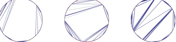
whereSθ is a random lamination of the disk called the stable lamination of parameterθ.
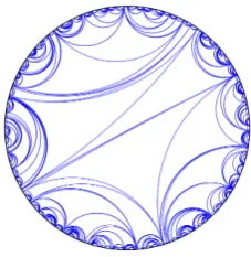
In the case θ = 2 the stable lamination of parameter 2 coincides with the Brownian triangulation. However whenθ <2, the random laminationSθis not a triangulation anymore and its complement inD
contains open polygons with infinitely many faces, see Fig. 4. Also, the dimension ofSθ equals
dim(Sθ) = 2−
1
θ.
The strategy of the proof of Theorem 2 follows roughly that of Theorem 1. The dual tree associated to
Dnq is now a Galton-Watson tree with offspring distributionq conditioned on havingn−1 leaves. This
particular conditioning of Galton-Watson trees has recently been studied in [18] (see also [21]) and in particular it has been shown [18] that the rescaled contour functions of the last trees converge towards the height process of a stable L´evy process (see [13] for the definition). The main difficulty that arises whenθ <2 is that these random excursion functions do not have distinct local minima (hypothesisHe)
3e.g. q
and thus the construction of last section breaks down. Still, it is possible to build the stable lamination from the stable height process in a way similar asLe is constructed frome, see [17] for more details.
Figure 4. Stable laminations with parameters1.1 (left),1.5(middle) and1.9(right). Sim-ulations realized by Igor Kortchemski.
Many distributional properties of the stable laminations are still to be calculated. E.g.:
Open question 2(I. Kortchemski). What is the distribution of the length of the longest diagonal ofSθfor θ∈(1,2)? The area of the largest face? What happens if the weight sequenceq={qi :i∈ {0,2,3,4, ...}}
is not a probability sequence or has infinite variance?
2.
Recursive triangulations
The results of this section come from [10] to which the reader is referred for details.
The last two sections studied the limit of n.c.c. under the uniform or “Boltzmann” type distributions. Another very natural probability measure, the recursive measure, arises when we actually try to draw a triangulation on a sheet of paper. A new object appears in the limit.
The recursive triangulation of Pn is the random discrete triangulation Rn obtained by the following
process. We start with the empty n-gon Pn and draw a uniform diagonal of it. Iteratively, we draw
a diagonal uniformly among those that do not intersect (inside D) the previous drawn diagonals. The
process stops after n−3 steps when no diagonal can be added to the configuration anymore. Although Rn =Tn in law forn= 3,4and5, the recursive and uniform triangulations differ much whennis large
and a new object appears in the limit:
Theorem 3 ( [10]). We have the following convergence in distribution fordH
Rn (d) −−−−→
n→∞ R.
The random lamination Ris a continuous triangulation called the random recursive triangulation of the disk. Although R roughly looks like the Brownian triangulation, they are very different and R is “fatter”
dim(R) = 1 +β∗, with β∗=
√
17−3
2 ≈0,56.
The recursive triangulation of the disk can be constructed directly as follows: we consider a sequence
U1, V1, U2, V2, . . . of independent random variables, which are uniformly distributed over the unit circle S1. We then construct inductively a sequence L1, L2, . . . of random closed subsets of the (closed) unit diskD. To begin with,L1just consists of the chord[U1V1]with endpointsU1andV1. Then at stepn+ 1, we consider two cases. Either the chord[Un+1Vn+1]intersectsLn, and we putLn+1=Ln. Or the chord
[Un+1Vn+1]does not intersect Ln, and we putLn+1=Ln∪[Un+1Vn+1]. Thus, for every integern≥1,
Ln is a disjoint union of random chords. We then letRto be the closure of the increasingLn’s:
R= [
n≥1
The tools used to study R are very different from the ones used in the last sections. However the scenario is the same: we try to understand the contour function of the dual tree associated to Ln and
prove a convergence of these contour processes (in a certain sense) towards a continuous non-negative process(mx: 0≤x≤1) which finally encodes the lamination via
R (d)= Lm, (7)
in the sense of (6). This coding of R by m then permits to deduce properties of R (e.g. Hausdorff dimension) from properties ofm(e.g. H¨older continuity exponent). Let us clarify the construction ofm. Forx∈[0,1]we define (see Fig. 5)
mn(x) := #{chords ofLn that intersect[1, e2iπx]}.
1
e2iπx
Figure 5. Definition ofmn(x)(four in this case).
This function plays the role of the contour function associated to the dual tree ofLn. It is then possible
to prove that for all x∈[0,1]we have the following convergence in probability
n−β∗/2mn(x) (P) −−−−→
n→∞ mx, (8)
where(mx: 0≤x≤1)is a continuous random excursion which is H¨older continuous of exponentβ∗−ε
for allε >0. Note that the last convergence is strictly weaker than a functional convergence in the type of (3):
n−β∗/2 mn(x)
x∈[0,1] −−−−→n→∞ (mx)x∈[0,1]
in probability for theL∞-norm over[0,1]. This convergence, conjecture in [10] has been recently proved by Nicolas Broutin and Henning Sulzbach [7]. Even without this strong convergence, it is still possible to prove (7). Let us mention that the main tool used to prove (8) is fragmentation theory, see [5]. In particular the exponent β∗ appears as the so-called Malthusian exponent of a fragmentation process intimately related to the construction ofR.
3.
R
-trees, dendrites and laminations
Before introducing our last character in the next section, we show that laminations can, in a sense, be considered as weak versions of continuous trees thus giving an alternative approach to the classical Gromov-Hausdorff topology.
3.1.
Laminations as limit of discrete trees
Question: (Q)Assume that(τn)n≥0is a sequence of random trees whose “size” grow to infinity with n. How can we make sense of a continuous limit of theτn?
Let us first remind the reader of the classical scaling limit approach to the last question based on the Gromov-Hausdorff topology: if(E, d)and(E0, d0)are two compact metric spaces, the Gromov-Hausdorff distance between them is
dGH (E, d),(E0, d0)
:= inf{dH φ(E), φ0(E0)
},
where the infimum is taken over all choices of a metric space (F, δ), isometric embeddingsφ : E → F
and φ0 :E0 →F wheredH denotes the Hausdorff distance in(F, δ). The Gromov-Hausdorff distance is indeed a distance on the set of equivalence classes of compact metric space (which is a Polish space). A discrete tree can obviously be seen as a metric space by endowing it with the graph metricdgr, hence an answer to(Q)is :
Answer 1: Find a scaling parameter αn and show that the rescaled (finite) random
compact metric space(τn, αn·dgr)converges in distribution fordGH.
The metric spaces arising as Gromov-Hausdorff limits of rescaled trees are known as R-trees. They are
compact metric spaces without cycles and such that the only geodesic between any two points is isometric to a real segment, see [19]. Several classes of random discrete trees have been investigated under that view point (Galton-Watson trees, Markov branching trees).
But this approach has a drawback: since the set of equivalence classes of compact metric spaces is not compact fordGH, one usually has to establish a thorny tightness property for the rescaledτn, even worse,
some very natural sequences of random trees are not tight for dGH.
Let us give another approach to(Q). Assume for simplicity that the discrete trees we are dealing with are rooted ordered discrete trees with no vertices of degree2. This class is particularly nice since it is in bijection with dissections of finite regular polygons as shown on Fig. 6. If τ is such a tree we denote by
1
2
3 4 5
6 7
8
Figure 6. A tree and its dual dissection.
Dis(τ) the dissection associated withτ. Viewing our random discrete treesτn through their associated
dissections then gives a new point of view to (Q):
Answer 2: Show that(Dis(τn))n≥1converges for the Hausdorff topology onD.
The continuous limit of the discrete random trees (τn) is now a random lamination. Within this
framework, the stable laminations of parameter θ ∈ [1,2] loosely speaking appear as the lamination limits of Galton-Watson trees whose offspring reproduction law is in the domain of attraction of a stable law of parameter θ. The great advantage of this approach lies in the compactness of the Hausdorff topology of D: we knowa priori that(Dis(τn))admits sub-sequential weak limits fordGH.
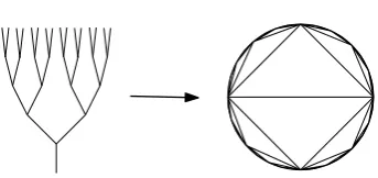
Let us give a trivial example. Considerτn the (deterministic) binary tree full up to leveln, see Fig. 7.
It is easy to see that the sequence τn cannot be rescaled to converge in the Gromov-Hausdorff sense
towards a continuousR-tree, however(τn)converges in the lamination sense towards the (deterministic)
lamination of Fig. 7.
Figure 7. A binary tree full up to level5and its lamination limit.
3.2.
Laminations as measured dendrites
As in the discrete setting, we will see that a lamination hides a “dual” topological tree. To simplify the exposition we present this construction in the case of the Brownian triangulation. The setting could be adapted to more general random laminations.
If Bis the Brownian triangulation we define an equivalence relation≈onD by puttingx≈y if and
only ifxandy belong to a chord of Bor if they both belong to the closure of a triangle of D\B. Since,
a.s. there are no triangles ofD\Bwhich are adjacent to eachother, the relation≈indeed is an equivalence
relation. We then consider the random topological quotient space
T = D/≈
endowed with the quotient topology. We write πfor the canonical projection. It is an exercise to check thatT a.s. is adendrite: a continuum (compact connected topological space) containing no simple closed curve. See [8] for a survey and for 32equivalent characterizations of dendrites. This “topological tree” can be seen as the dual ofB. WhenB=Le thenT is homeomorphic to the Brownian treeTecoded by e, see [20]. Unfortunately, we conjecture that in the Brownian case this topology is constant:
Open question 4 (Topology of Aldous’ CRT). The topology of T is almost surely constant, i.e. two independent samples of the Brownian CRT are almost surely homeomorphic.
But the lamination contains more information than this dendrite. Indeed, the push-forward byπof the uniform measure on S1 endows the dendriteT with a Borel probability measureµ. Also, the clockwise ordering ofS1\{1}leads to a lexicographical order≺overT given bya≺bif and only if
inf
s∈[0,1) :π(e2iπs) =a <inf
t∈[0,1) :π(e2iπt) =b .
Actually, it is a simple but tedious exercise to see that in the Brownian case the information provided by the laminationB and(T, µ,≺, π(1)) are equivalent, in other words one can reconstructBfrom (T, µ,≺
, π(1)).
4.
The Markovian hyperbolic triangulation
The results of this section come from [11] to which the reader is referred for details.
We finish this expository paper by introducing the Markovian hyperbolic triangulationH. This con-tinuous triangulation differs much from the previous ones and is related to hyperbolic geometry. In fact, contrary toB,SθorR, the continuous triangulationHis not introduced as a limit of discrete n.c.c. neither it is constructed as a lamination associated with an excursion process in the sense of (6). Consequently it has no clearly defined continuousR-tree associated with it.
In this section we have to work with hyperbolic geometry. The definition of lamination (and continuous triangulation) is slightly changed by considering hyperbolic chords instead of Euclidean ones. See Fig. 8. All the objects are denoted with an additional h- for “hyperbolic”.
Figure 8. A continuous triangulation with Euclidean chords and its h-version.
h-triangle with its three apexes located on the boundary at infinity ∂D, such a triangle is called ideal. We recall that the M¨obius group Mob of all hyperbolic isometries acts transitively on the set of ideal triangles. In other words, all the triangles of a maximal h-triangulation are conformally equivalent and can be all seen as the same tiles!
In view of these remarks, it is legitimate to ask if there exists a random h-triangulationT whose law is invariant under the action ofMobthat is,T =φ(T)in distribution for everyφ∈Mob. The answer is positive and it is fairly easy to construct many examples, see [11]. However there is an essentially unique random h-triangulation that isMob-invariant and satisfies a spatial Markov property that can be roughly described as follows:
Spatial Markov Property : Given a triangle T = (abc) in T, the triangulation re-stricted to the three connected components of the complement ofT inDare conditionally
independent, and moreover, the part that is beyond (bc) is independent of the position ofa.
Theorem 4 ( [11]). There is a unique (law of a) random h-triangulationHsuch that
• the union of the triangles ofHis of full Lebesgue measure in D, • φ(H) =H in distribution for everyφ∈Mob,
• Hsatisfies the above spatial Markov property.
The triangulationHis constructed in [11] using basic hyperbolic tools and subordinators. Although not locally finite (they are no triangles adjacent to each other), it is the thinest of all laminations considered in this paper in the sense that
dim(H) = 1.
Many open questions about this object remain open:
Open question 5 ( [11]). Is there a “natural” random discrete n.c.c. model that converges towardsH? Is there a random R-tree dual toHas the Brownian tree or stable trees are dual toB andSθ?
References
[1] D. Aldous,The continuum random tree III, Ann. Probab., 21 (1993), pp. 248–289.
[2] ,Recursive self-similarity for random trees, random triangulations and Brownian excursion., Ann. Probab., 22 (1994), pp. 527–545.
[3] D. Aldous,Triangulating the circle, at random., Amer. Math. Monthly, 101 (1994).
[4] N. Bernasconi, K. Panagiotou, and A. Steger,On properties of random dissections and triangulations, in Proceed-ings of the Nineteenth Annual ACM-SIAM Symposium on Discrete Algorithms, New York, 2008, ACM, pp. 132–141. [5] J. Bertoin,Random Fragmentations and Coagulation Processes, no. 102 in Cambridge Studies in Advanced
Mathe-matics, Cambridge University Press, 2006.
[6] F. Bonahon,Geodesic laminations on surfaces, in Laminations and foliations in dynamics, geometry and topology (Stony Brook, NY, 1998), vol. 269 of Contemp. Math., Amer. Math. Soc., Providence, RI, 2001, pp. 1–37.
[7] N. Broutin and H. Sulzbach,The dual tree of a recursive triangulation of the disk, (2012).
[8] J. J. Charatonik and W. J. Charatonik, Dendrites, in XXX National Congress of the Mexican Mathematical Society (Spanish) (Aguascalientes, 1997), vol. 22 of Aportaciones Mat. Comun., Soc. Mat. Mexicana, M´exico, 1998, pp. 227–253.
[9] N. Curien and I. Kortchemski,Random non-crossing plane configurations: a conditioned Galton-Watson tree ap-proach, Random Structures and Algorithms (to appear).
[10] N. Curien and J.-F. Le Gall,Random recursive triangulations of the disk via fragmentation theory, Ann. Probab., 39 (2011), pp. 2224–2270.
[11] N. Curien and W. Werner,The Markovian hyperbolic triangulation, J. Eur. Math. Soc., 15 (2013), pp. 1309–1341. [12] L. Devroye, P. Flajolet, F. Hurtado, and W. Noy, M.and Steiger,Properties of random triangulations and
trees., Discrete Comput. Geom., 22 (1999).
[13] T. Duquesne and J.-F. Le Gall,Random trees, L´evy processes and spatial branching processes, Ast´erisque, (2002), pp. vi+147.
[14] P. Flajolet and M. Noy,Analytic combinatorics of non-crossing configurations, Discrete Math., 204 (1999), pp. 203– 229.
[15] Z. Gao and L. B. Richmond,Root vertex valency distributions of rooted maps and rooted triangulations, European J. Combin., 15 (1994), pp. 483–490.
[16] B. Haas and G. Miermont,Scaling limits of Markov branching trees, with applications to Galton-Watson and random unordered trees, Ann. of Probab., 40 (2012), pp. 2589–2666.
[17] I. Kortchemski,Random stable laminations of the disk, Ann. Probab.(to appear).
[18] ,Invariance principles for Galton-Watson trees conditioned on the number of leaves, Stoch. Proc. Appl., 122 (2012), pp. 3126–3172.
[19] J.-F. Le Gall,Random real trees, Ann. Fac. Sci. Toulouse Math. (6), 15 (2006), pp. 35–62.
[20] J.-F. Le Gall and F. Paulin,Scaling limits of bipartite planar maps are homeomorphic to the 2-sphere, Geom. Funct. Anal., 18 (2008), pp. 893–918.
[21] D. Rizzolo,Scaling limits of Markov branching trees and Galton-Watson trees conditioned on the number of vertices with out-degree in a given set, arXiv:1105.2528, (2011).