Finding Common Weights in Two-Stage Network DEA

(1)

Int. J. Data Envelopment Analysis (ISSN 2345-458X)

Vol.5, No.4, Year 2017 Article ID IJDEA-00422, 16 pages Research Article

Finding Common Weights in Two-Stage

Network DEA

M. khazraei1, M.R. Mozaffari*2

(1,2) _{Department of mathematic, Shiraz branch, Islamic Azad university, Shiraz, Iran.}

Received 07 April 2017, Accepted 12 August 2017

Abstract

In data envelopment analysis (DEA), multiplier and envelopment CCR models evaluate the decision-making units (DMUs) under optimal conditions. Therefore, the best prices are allocated to the inputs and outputs. Thus, if a given DMU was not efficient under optimal conditions, it would not be considered efficient by any other models. In the current study, using common weights in DEA, a number of decision-making units are evaluated under the same conditions, and a number of two-stage network DEA models are proposed within the framework of multi-objective linear programming (MOLP) for finding common weights. Furthermore, using the infinity norm, common weight sets are determined in two-stage network models with MOLP structures.

Keywords: data envelopment analysis, common weights, ranking, two-stage network, decision-making unit.

*. Corresponding author Email: [email protected]

(2)

1. Introduction

Data envelopment analysis (DEA) is a method for measuring the performance of decision-making units (DMUs) that consume multiple inputs to produce multiple outputs. Two basic DEA models, namely CCR and BCC, have become the standard for performance evaluation under assumptions of constant (CRS) and variable returns to scale (VRS). DEA often deals with single-stage production processes in which the internal structure of DMUs is not taken into account. On the other hand, network DEA involves multi-stage processes, where the basic structure, which shows the trend of intermediate measures in-between stages, plays a critical role. Fare and Grosskopf (1996) were among the first to study efficiency in such processes within the framework of a model for analyzing network activity. Castelli et al. (2010) provided a comprehensive and categorized overview of the models and methods developed for various configurations of multi-stage production. Kao (2014), presented a full categorization of the literature on data envelopment analysis based on network structure type and applied model, where the same weights were allocated to intermediate measures, regardless of whether the measures were considered the outputs of the first stage or the inputs of the second stage. Liang et al. (2008) and Cook et al. (2010) studied efficiency evaluation in two-stage processes using theoretical concepts. Kao et al. (2014) used a multi-objective programming method for efficiency evaluation in network structures. Recently, Despotis et al. (2014) introduced a combined method of efficiency measurement in two-stage networks, in which the efficiency of each stage was estimated first, and then the overall efficiency was obtained on that basis. However, the weakness of this method is that it cannot be easily extended to multi-stage network processes. The current research focuses on the different

orientations selected for stages one and two of a two-stage network, which are technically created in order to simplify the models and keep them within the field of linear programming. In this study, two-stage network processes are discussed with focus on a variety of distinct processes covering all possible configurations.

2. Preliminaries

This section provides the basic concepts of the two-stage network in data envelopment analysis.

Consider 𝑛 decision-making units, denoted by the subscript 𝑗 (DMUj), that use 𝑚 input vectors Xj for consumption in the first stage. The vector Zj with 𝑞

elements is used as the output of stage one and the input of stage two in the DEA network.

Yj=(yrj , r=1,…,s): Vector of final outputs in DMUj with the weight vector U=(𝑢1,…, 𝑢𝑠).

Lj=(ldj , d=1,…,a): Vector of external inputs in DMUj with the weight vector H=(ℎ1,…, ℎ𝑎).

Kj=(kcj , c=1,…,b): Vector of external outputs in DMUj with the weight vector T=(𝑡1,…, 𝑡𝑏).

𝑒_𝑗𝑜: Overall efficiency of DMUj

𝑒_𝑗1: Efficiency of stage one in DMUj

𝑒_𝑗𝑜: Efficiency of stage two in DMUj Consider the case where we have X inputs, Y outputs, and Z intermediate measures, with no external inputs or outputs. In this case, the efficiency of stages one and two are defined as follows:

𝑒𝑗1=

∑𝑞𝑝=1𝑧𝑝𝑗𝑤𝑝

∑𝑚𝑖=1𝑥𝑖𝑗𝑣𝑖

, _𝑒

𝑗2=

∑𝑠_𝑟=1𝑦_𝑟𝑗𝑢_𝑟 ∑𝑞𝑝=1𝑧𝑝𝑗𝑤𝑝

and the overall efficiency of DMUj is calculated as:

𝑒_𝑗2=∑ 𝑦𝑟𝑗

𝑠 𝑟=1 𝑢𝑟

∑𝑚𝑖=1𝑥𝑖𝑗𝑣𝑖.

(3)

1437

Max ∑ 𝑧𝑝𝑜

𝑞

𝑝=1 𝑤𝑝

∑𝑚𝑖=1𝑥𝑖𝑜𝑣𝑖

s.t: ∑𝑞𝑝=1𝑧𝑝𝑗𝑤𝑝− ∑𝑚𝑖=1𝑥𝑖𝑗𝑣𝑖 ≤ 0 , 𝑗 = 1, … , 𝑛 (1)

𝑣𝑖 ≥ ℇ , i=1,…,m 𝑤𝑝 ≥ ℇ , p=1,…,q

The DEA model for efficiency evaluation in the second network stage is formulated as follows:

Max ∑𝑠𝑟=1𝑦𝑟𝑜𝑢𝑟

∑𝑞𝑝=1𝑧𝑝𝑜𝑤𝑝

s.t: ∑𝑠𝑟=1𝑦𝑟𝑗𝑢𝑟 − ∑𝑞𝑝=1𝑧𝑝𝑗𝑤𝑝 ≤ 0 , 𝑗 = 1, … , 𝑛 (2)

𝑢𝑟 ≥ ℇ , r=1,…,s 𝑤𝑝 ≥ ℇ , p=1,…,q

By adding the restriction of Model (1) to Model (2) and vice versa, we will arrive at Models (3) and (4), respectively (Despotis et al., 2014).

𝑞

𝑝=1 𝑤𝑝

∑𝑚𝑖=1𝑥𝑖𝑜𝑣𝑖

s.t: ∑𝑞𝑝=1𝑧𝑝𝑗𝑤𝑝− ∑𝑚𝑖=1𝑥𝑖𝑗𝑣𝑖 ≤ 0 , 𝑗 = 1, … , 𝑛

∑𝑠𝑟=1𝑦𝑟𝑗𝑢𝑟− ∑𝑞𝑝=1𝑧𝑝𝑗𝑤𝑝 ≤ 0 ,

𝑗 = 1, … , 𝑛 (3) 𝑣𝑖≥ ℇ , i=1,…,m

𝑢𝑟 ≥ ℇ , r=1,…,s 𝑤𝑝 ≥ ℇ , p=1,…,q

The linear form of Model (3) is as follows: Max ∑𝑞𝑝=1𝑧𝑝𝑜𝑤𝑝

s.t: ∑𝑚𝑖=1𝑥𝑖𝑜𝑣𝑖 = 1

∑𝑞𝑝=1𝑧𝑝𝑗𝑤𝑝− ∑𝑚𝑖=1𝑥𝑖𝑗𝑣𝑖 ≤ 0 ,

j=1,…,n (4) ∑𝑠𝑟=1𝑦𝑟𝑗𝑢𝑟− ∑𝑞𝑝=1𝑧𝑝𝑗𝑤𝑝 ≤ 0 ,

j=1,…,n

𝑣𝑖 ≥ ℇ , i=1,…,m 𝑢𝑟 ≥ ℇ , r=1,…,s 𝑤𝑝 ≥ ℇ , p=1,…,q

Model (5) is used to calculate efficiency in the second stage (Despotis et al., 2014).

Max ∑𝑠𝑟=1𝑦𝑟𝑜𝑢𝑟

s.t: ∑𝑞𝑝=1𝑧𝑝𝑗𝑤𝑝− ∑𝑚𝑖=1𝑥𝑖𝑗𝑣𝑖 ≤ 0 , 𝑗 = 1, … , 𝑛 (5) ∑𝑠𝑟=1𝑦𝑟𝑗𝑢𝑟− ∑𝑞𝑝=1𝑧𝑝𝑗𝑤𝑝 ≤ 0 , 𝑗 = 1, … , 𝑛

𝑣𝑖 ≥ ℇ , i=1,…,m

𝑢𝑟 ≥ ℇ , r=1,…,s

𝑤𝑝 ≥ ℇ , p=1,…,q

Model (6) is the linear form of Model (5). Max ∑𝑠𝑟=1𝑦𝑟𝑜𝑢𝑟

s.t: ∑𝑞𝑝=1𝑧𝑝𝑜𝑤𝑝 = 1

∑𝑞𝑝=1𝑧𝑝𝑗𝑤𝑝 − ∑𝑚𝑖=1𝑥𝑖𝑗𝑣𝑖 ≤ 0

j=1,…,n (6) ∑𝑠𝑟=1𝑦𝑟𝑗𝑢𝑟− ∑𝑞𝑝=1𝑧𝑝𝑗𝑤𝑝 ≤ 0 ,

j=1,…,n

𝑣𝑖 ≥ ℇ , i=1,…,m

𝑢𝑟 ≥ ℇ , r=1,…,s

𝑤𝑝 ≥ ℇ , p=1,…,q

Models (3) and (5) have common restrictions; thereby, the following can be formulated: (see Despotis et al. (2016))

𝑞

𝑝=1 𝑤𝑝

∑𝑚_𝑖=1𝑥_𝑖𝑜𝑣_𝑖

Max ∑ 𝑦𝑟𝑜

𝑠 𝑟=1 𝑢𝑟

s.t: ∑𝑞𝑝=1𝑧𝑝𝑗𝑤𝑝− ∑𝑚𝑖=1𝑥𝑖𝑗𝑣𝑖≤ 0 , 𝑗 = 1, … , 𝑛 (7) ∑𝑠𝑟=1𝑦𝑟𝑗𝑢𝑟− ∑𝑞𝑝=1𝑧𝑝𝑗𝑤𝑝 ≤ 0 , 𝑗 = 1, … , 𝑛

𝑣𝑖 ≥ ℇ , i=1,…,m 𝑢𝑟 ≥ ℇ , r=1,…,s 𝑤𝑝 ≥ ℇ , p=1,…,q

Model (7) is a bi-level linear programming problem, in which two objective functions apply the restrictions of stages one and two in the DEA network.

3. Two-stage Network Processes

(4)

network DEA, a number of models are proposed for finding common weight sets.

3.1. Configuration One

In this configuration, the outputs of stage one are inputs in stage two, as illustrated in Fig. 1.

A) In stage one, X = (𝑥1,…,𝑥𝑚) is the input

vector with the weight vector V=(𝑣1,…,𝑣𝑚), and Z=(𝑧1,…,𝑧𝑞) is the

output vector with the weight vector W=(𝑤1,…, 𝑤𝑞). To find a common weight

set and rank the DMUs in this stage, we first use the following model: (see Despotis et al. (2016))

Ecsw1: Min ∑𝑛𝑗=1(∑𝑚𝑖=1𝑥𝑖𝑗𝑣𝑖− 𝑚 − ∑𝑞𝑝=1𝑧𝑝𝑗𝑤𝑝+ 𝑛)

s.t: m- ∑𝑚𝑖=1𝑥𝑖𝑗𝑣𝑖 ≤ 0 ,

j=1,…,n

n− ∑𝑞𝑝=1𝑧𝑝𝑗𝑤𝑝 ≥ 0 ,

j=1,…,n (8)

j=1,…,n

𝑣𝑖 ≥ ℇ , i=1,…,m 𝑤𝑝 ≥ ℇ , p=1,…,q

m , n ≥0

where, m=min

1≤𝑗≤𝑛∑ 𝑥𝑖𝑗

𝑚

𝑖=1 𝑣𝑖,

n=max

1≤𝑗≤𝑛∑ 𝑧𝑝𝑗

𝑞

𝑝=1 𝑤𝑝, and ℰ is the smallest

positive number.

B) For the purposes of calculating a common weight set in the second network stage, Model (9) is suggested:

Ecsw2: Min ∑𝑛_𝑗=1(∑𝑞𝑝=1𝑧𝑝𝑗𝑤𝑝− 𝑀 − ∑𝑠𝑟=1𝑦𝑟𝑗𝑢𝑟+ 𝑁)

s.t: M-∑𝑞𝑝=1𝑧𝑝𝑗𝑤𝑝 ≤ 0 ,

j=1,…,n

N− ∑𝑠𝑟=1𝑦𝑟𝑗𝑢𝑟 ≥ 0 ,

j=1,…,n

j=1,…,n (9) 𝑢𝑟 ≥ ℇ , r=1,…,s

𝑤𝑝 ≥ ℇ , p=1,…,q

M , N ≥0

In Model (9), M and N are defined as follows:

M=min

𝑞

𝑝=1 𝑤𝑝

N=max

1≤𝑗≤𝑛∑ 𝑦𝑟𝑗

𝑠

𝑟=1 𝑢𝑟

Similarly, Model (6) denoted by Eefficiency2 is used for efficiency calculation in the second network stage.

To calculate the overall efficiency of the system, we use the following formula: Eoverall: Min ∑𝑛𝑗=1(∑𝑚𝑖=1𝑥𝑖𝑗𝑣𝑖− m − ∑𝑞𝑝=1𝑧𝑝𝑗𝑤𝑝 + n) + ∑𝑗=1𝑛 (∑𝑞𝑝=1𝑧𝑝𝑗𝑤𝑝− 𝑀 − ∑𝑠𝑟=1𝑦𝑟𝑗𝑢𝑟+ N)

s.t: m − ∑𝑚𝑖=1𝑥𝑖𝑗𝑣𝑖≤ 0 ,

j=1,…,n

𝑛 − ∑𝑞𝑝=1𝑧𝑝𝑗𝑤𝑝 ≥ 0 ,

j=1,…,n

𝑀 − ∑𝑞𝑝=1𝑧𝑝𝑗𝑤𝑝 ≤ 0 ,

j=1,…,n (10)

N − ∑𝑠𝑟=1𝑦𝑟𝑗𝑢𝑟 ≥ 0 ,

j=1,…,n

∑𝑞𝑝=1𝑧𝑝𝑗𝑤𝑝 − ∑𝑚𝑖=1𝑥𝑖𝑗𝑣𝑖≤ 0 ,

j=1,…,n

𝑣𝑖 ≥ ℇ , i=1,…,m

𝑢𝑟 ≥ ℇ , r=1,…,s

𝑤𝑝 ≥ ℇ , p=1,…,q

m , 𝑛, 𝑀, N ≥ 0

3.2. Configuration Two

1

2 X

Z

(5)

1439

1

2 X

Z

L

Y

Figure 2. Two-stage network configuration two In this case, an external input enters the

system in stage two, as can be seen in Fig. 2:

A) In stage one, the inputs and outputs are similar to the previous configuration, and thus, the formulas (8) and (4) denoted by ecsw1 and eefficiency2, respectively, are successively used for the purposes of unit ranking.

B) In the second stage, we have the input vectors Z=(𝑧1,…,𝑧𝑞) and L=(𝑙1,…,𝑙𝑎)

with the weight vectors W=(𝑤1,…, 𝑤𝑞)

and H=(ℎ1,…, ℎ𝑎), respectively, and the

output vector Y = (𝑦1,…,𝑦𝑠) with the

weight vector U=(𝑢1,…, 𝑢𝑠). For

efficiency calculation with common weights, Model (11) is first employed: ecsw2: Min ∑𝑛_𝑗=1(∑𝑞𝑝=1𝑧𝑝𝑗𝑤𝑝 − 𝑀1+ ∑𝑎𝑑=1𝑙𝑑𝑗ℎ𝑑− 𝑀2− ∑𝑠𝑟=1𝑦𝑟𝑗𝑢𝑟 + 𝑁)

s.t: 𝑀1− ∑𝑞𝑝=1𝑧𝑝𝑗𝑤𝑝 ≤ 0 ,

j=1,…,n

𝑀2− ∑𝑎𝑑=1𝑙𝑑𝑗ℎ𝑑≤ 0 ,

j=1,…,n

N− ∑𝑠𝑟=1𝑦𝑟𝑗𝑢𝑟 ≥ 0 ,

j=1,…,n (11)

∑𝑠𝑟=1𝑦𝑟𝑗𝑢𝑟− ∑𝑞𝑝=1𝑧𝑝𝑗𝑤𝑝 − ∑𝑎𝑑=1𝑙𝑑𝑗ℎ𝑑≤ 0 ,

j=1,…,n

𝑢𝑟 ≥ ℇ , r=1,…,s

𝑤𝑝 ≥ ℇ , p=1,…,q

ℎ𝑑≥ ℇ , d=1,…,a

𝑀1 , 𝑀2, N ≥0

In this model,

M1=min

𝑞

𝑝=1 𝑤𝑝,

M2=min

1≤𝑗≤𝑛∑ 𝑙𝑑𝑗ℎ𝑑

𝑎

𝑑=1 , and

N=max

1≤𝑗≤𝑛∑ 𝑦𝑟𝑗

𝑠

𝑟=1 𝑢𝑟.

Then, the following model is presented in accordance with Model (6) for efficiency calculation in this case:

eefficiency2: Max ∑𝑠𝑟=1𝑦𝑟𝑜𝑢𝑟

s.t: ∑𝑞𝑝=1𝑧𝑝𝑜𝑤𝑝+ ∑𝑎𝑑=1𝑙𝑑𝑜ℎ𝑑 = 1

j=1,…,n (12)

j=1,…,n

𝑣𝑖 ≥ ℇ , i=1,…,m

𝑢𝑟 ≥ ℇ , r=1,…,s

𝑤𝑝 ≥ ℇ , p=1,…,q

ℎ𝑑≥ ℇ , d=1,…,a

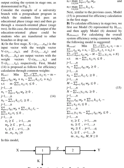
The following linear programming model is proposed for calculating a common weight set in the overall system within the framework of two-stage network DEA. eefficiency2: Max ∑𝑠𝑟=1𝑦𝑟𝑜𝑢𝑟

s.t: ∑𝑞𝑝=1𝑧𝑝𝑜𝑤𝑝+ ∑𝑎𝑑=1𝑙𝑑𝑜ℎ𝑑 = 1

∑𝑞𝑝=1𝑧𝑝𝑗𝑤𝑝 − ∑𝑚𝑖=1𝑥𝑖𝑗𝑣𝑖 ≤ 0

j=1,…,n

j=1,…,n (13) 𝑣𝑖 ≥ ℇ , i=1,…,m

𝑢𝑟 ≥ ℇ , r=1,…,s

𝑤𝑝 ≥ ℇ , p=1,…,q

(6)

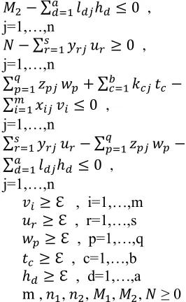
3.3. Configuration Three

In this configuration, there is one external output exiting the system in stage one, as demonstrated in Fig. 3.

Consider the example of a university branch with a postgraduate program in which the students first pass an educational phase (stage one) and then go through a research-oriented phase (stage two). In this case, the external output of the education-oriented phase could be students who are transferred to other branches or drop out.

A) In the first stage, X = (𝑥1,…,𝑥𝑚) is the

input vector with the weight vector V=(𝑣1,…,𝑣𝑚), and Z=(𝑧1,…,𝑧𝑞) and

K=(𝑘1,…,𝑘𝑏) are output vectors with the

weight vectors U=(𝑢1,…, 𝑢𝑠) and

T=(𝑡1,…, 𝑡𝑏), respectively. First, Model

(14) is proposed as follows for efficiency calculation through common weights: Hcsw1: Min ∑𝑛_𝑗=1(∑𝑚𝑖=1𝑥𝑖𝑗𝑣𝑖− m − ∑𝑞𝑝=1𝑧𝑝𝑗𝑤𝑝+ 𝑛1− ∑𝑏𝑐=1𝑘𝑐𝑗𝑡𝑐 + 𝑛2)

s.t: m -∑𝑚𝑖=1𝑥𝑖𝑗𝑣𝑖 ≤ 0 ,

j=1,…,n

𝑛1− ∑𝑞𝑝=1𝑧𝑝𝑗𝑤𝑝 ≥ 0 ,

j=1,…,n (14)

𝑛2− ∑𝑏𝑐=1𝑘𝑐𝑗𝑡𝑐 ≥ 0 ,

j=1,…,n

∑𝑞𝑝=1𝑧𝑝𝑗𝑤𝑝+ ∑𝑏𝑐=1𝑘𝑐𝑗𝑡𝑐− ∑𝑚𝑖=1𝑥𝑖𝑗𝑣𝑖 ≤ 0 ,

j=1,…,n

𝑣𝑖≥ ℇ , i=1,…,m

𝑤𝑝 ≥ ℇ , p=1,…,q

𝑡𝑐 ≥ ℇ , c=1,…,b

m , 𝑛1, 𝑛2 ≥0

In this model,

m=min

1≤𝑗≤𝑛∑ 𝑥𝑖𝑗

𝑚

𝑖=1 𝑣𝑖,

n1=max

𝑞

𝑝=1 𝑤𝑝, and

n2=max

1≤𝑗≤𝑛∑ 𝑘𝑐𝑗

𝑏

𝑐=1 𝑡𝑐.

Next, similar to the previous cases, Model (15) is presented for efficiency calculation in the first stage.

B) To calculate efficiency in stage two, we first use Model (9) represented by Hcsw2, and then apply Model (6) denoted by Hefficiency2. For calculating the overall system efficiency using common weights, the following model is suggested:

Hoverall: Min ∑𝑛 (

𝑗=1 ∑𝑚𝑖=1𝑥𝑖𝑗𝑣𝑖− m −

∑ 𝑧𝑝𝑗 𝑞

𝑝=1 𝑤𝑝+ 𝑛1− ∑𝑏𝑐=1𝑘𝑐𝑗𝑡𝑐+ 𝑛2) +

∑𝑛 (

𝑗=1 ∑ 𝑧𝑝𝑗 𝑞

𝑝=1 𝑤𝑝− 𝑀 − ∑𝑠𝑟=1𝑦𝑟𝑗𝑢𝑟+ 𝑁) s.t: m − ∑𝑚𝑖=1𝑥𝑖𝑗𝑣𝑖≤ 0 ,

j=1,…,n

𝑛2− ∑𝑏𝑐=1𝑘𝑐𝑗𝑡𝑐 ≥ 0 ,

j=1,…,n

𝑀 − ∑𝑞𝑝=1𝑧𝑝𝑗𝑤𝑝 ≤ 0 ,

j=1,…,n (15)

𝑁 − ∑𝑠𝑟=1𝑦𝑟𝑗𝑢𝑟 ≥ 0 ,

j=1,…,n

∑𝑞𝑝=1𝑧𝑝𝑗𝑤𝑝 + ∑𝑏𝑐=1𝑘𝑐𝑗𝑡𝑐− ∑𝑚𝑖=1𝑥𝑖𝑗𝑣𝑖 ≤ 0 ,

j=1,…,n

𝑣𝑖 ≥ ℇ , i=1,…,m

𝑢𝑟 ≥ ℇ , r=1,…,s

𝑤𝑝 ≥ ℇ , p=1,…,q

𝑡𝑐≥ ℇ , c=1,…,b

m , 𝑛1, 𝑛2, 𝑀, 𝑁 ≥ 0

1 K

Z

Figure 3. Two-stage network configuration three

Y

(7)

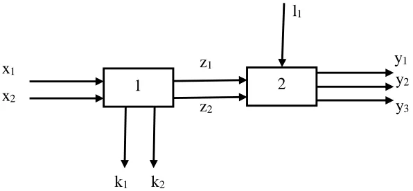
1441

3.4. Configuration Four

In this case, an output exits the system in stage one and an input enter the network in stage two; refer to the following figure4: A) The inputs and outputs in stage one are similar to the case of the third configuration. Therefore, we first make use of Model (14) denoted by hcsw1, and then apply Model (15) under the title of hefficiency1.

B) Similarly, in stage two, we successively use Models (11) and (12) represented by hcsw2 and hefficiency2, respectively. The following model is proposed for calculating a common weight set in the overall system:

hoverall: Min ∑𝑛_𝑗=1(∑𝑚𝑖=1𝑥𝑖𝑗𝑣𝑖− m − ∑𝑞𝑝=1𝑧𝑝𝑗𝑤𝑝+ 𝑛1− ∑𝑏𝑐=1𝑘𝑐𝑗𝑡𝑐 + 𝑛2) + ∑𝑛_𝑗=1(∑𝑞𝑝=1𝑧𝑝𝑗𝑤𝑝− 𝑀1+ ∑𝑎𝑑=1𝑙𝑑𝑗ℎ𝑑− 𝑀2− ∑𝑠𝑟=1𝑦𝑟𝑗𝑢𝑟 + 𝑁)

s.t m − ∑𝑚𝑖=1𝑥𝑖𝑗𝑣𝑖 ≤ 0 ,

j=1,…,n

𝑛2− ∑𝑏𝑐=1𝑘𝑐𝑗𝑡𝑐 ≥ 0 , 𝑀1− ∑𝑞𝑝=1𝑧𝑝𝑗𝑤𝑝≤ 0 ,

j=1,…,n (16)

𝑀2− ∑𝑎𝑑=1𝑙𝑑𝑗ℎ𝑑≤ 0 ,

j=1,…,n

𝑁 − ∑𝑠𝑟=1𝑦𝑟𝑗𝑢𝑟 ≥ 0 ,

j=1,…,n

∑𝑞𝑝=1𝑧𝑝𝑗𝑤𝑝 + ∑𝑏𝑐=1𝑘𝑐𝑗𝑡𝑐− ∑𝑚𝑖=1𝑥𝑖𝑗𝑣𝑖 ≤ 0 ,

j=1,…,n

𝑣𝑖 ≥ ℇ , i=1,…,m

𝑢𝑟 ≥ ℇ , r=1,…,s

𝑤𝑝 ≥ ℇ , p=1,…,q

𝑡𝑐≥ ℇ , c=1,…,b

ℎ𝑑≥ ℇ , d=1,…,a

m , 𝑛1, 𝑛2, 𝑀1, 𝑀2, 𝑁 ≥ 0

4. Numerical Example

Example 1: In this section, 40 university branches are considered as two-stage networks, each having two inputs and two outputs in the first stage and two inputs and three outputs in the second stage along with one external input and two external outputs as follows: (figure 5)

1 Z

Y

X

2 K

(8)

Table 1 provides the data on the 40 university branches under study. In this example, the inputs and outputs are defined as follows:

Stage one: Education-oriented phase of the postgraduate program

Stage Two: Research-oriented phase of the postgraduate program

X1: Number of admissions with an

entrance exam.

X2: Number of admissions without an

entrance exam

Z1: Number of graduates from the

education-oriented phase with an average of A

Z2: Number of graduates from the

education-oriented phase with an average of B

Y1: Number of graduates from the

research-oriented phase without a research article

research-oriented phase defending their research article

research-oriented phase with a research article published in an ISI-indexed journal L1: Number of guest students in the

research-oriented phase

K1: Number of expelled students

K2: Number of drop-out students

Efficiency evaluations were performed for the first two-stage network configuration using Models (4), (6), (8),

(9), and (10), the results of which can be observed in Table 2.

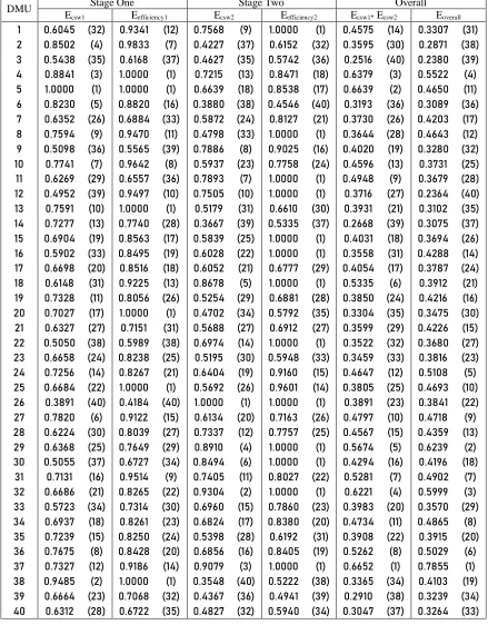
In Table 2, by comparing Ecsw1 and Eefficiency1 in the education-oriented phase, it can be observed that only one university branch is efficient in Ecsw1, while Eefficiency1 has deemed 6 branches as efficient. Furthermore, in the research-oriented stage, Ecsw2 presents one efficient unit, while 13 units are efficient according to Eefficiency2. In other words, in a comparison of units under similar conditions, Eefficiency would consider a smaller number of units as efficient comparing to Ecsw, as Eefficiency evaluates the units based on their optimal condition, while Ecsw determines efficiency scores for unit ranking under the same condition.

Referring to Table 2, it can be said that Branch 5 has done very well in the education-oriented phase, but was not efficient in the research-oriented stage. Moreover, the branch is overall inefficient according to Ecsw1* Ecsw2.

Unit 9 was not efficient in any of the stages or in the overall evaluation.

Unit 13 has performed well in the education-oriented phase based on Eefficiency1, and is considered efficient, but the unit is not efficient in the research-oriented phase or in the overall evaluation. Unit 22 is inefficient in the education-oriented stage, but it had an efficient performance in the research-oriented

1

2 k

1

Figure 5. Inputs and outputs in stage one

y

1

z

1

x

1

l

1

k

2

x

2

z

2

(9)

1443

phase; however, the unit is not overall efficient.

Unit 37 is not efficient in the education-oriented stage, but had performed efficiently in the research-oriented phase. The unit is considered overall efficient based on the column Ecsw1* Ecsw2.

Efficiency scores were calculated for the second two-stage network configuration using Models (4), (8), (11), (12), and (13). The results are provided in Table 3. In Table 3, ecsw1 has one efficient unit in the education-oriented phase, while eefficiency1 considers 6 units as efficient in this stage. In the research-oriented phase, ecsw2 deems one unit as efficient and eefficiency2 has 24 efficient units.

According to Table 3, Unit 5 is efficient in the education-oriented stage, while being efficient in the research-oriented phase. The unit is, however, efficient based on the overall evaluation.

Unit 8 is inefficient in the education-oriented phase and efficient in the research-oriented phase, and it is overall inefficient.

Unit 13 is efficient in both education- and research-oriented stages according to eefficiency1 and eefficiency2, respectively; however, the unit is deemed overall inefficient.

Unit 19 is not efficient in the first stage, but it is efficient in the research-oriented phase based on eefficiency2. Nevertheless, the unit is overall inefficient.

In the following, Figures 8 and 9 illustrate comparisons between the two methods in stages one and two, respectively.

Table 4 presents the efficiency scores calculated for the third network configuration using Models (6), (9), (14), (15), and (16).

In Table 4, 2 units are efficient based on Hcsw1 and 28 units are efficient based on Hefficiency1 in the education-oriented phase, while in the research-oriented stage, one

unit is efficient according to Hcsw1 and 13 units are efficient in Hefficiency2.

Based on Table 4, Unit 4 is efficient in the education-oriented stage, while it is considered inefficient in the research-oriented phase and the overall evaluation. Unit 9 is efficient in the first stage, but it is not efficient in the second stage, neither is it overall efficient.

Unit 26 is efficient in the education-oriented phase based on eefficiency1. The unit is also efficient in stage two and the overall evaluation.

Unit 38 is efficient in the education-oriented stage according to eefficiency1, but it is neither efficient in the research-oriented stage nor the overall evaluation.

The efficiency values measured for the fourth configuration through Models (11), (12), (14), (15), and (17) can be observed in Table 5.

Unit 9 is efficient in the education-oriented phase but inefficient in the research-oriented stage and the overall evaluation. Unit 29 is efficient in both education- and research-oriented stages according to hefficiency1 and hefficiency2, respectively. The unit is also overall efficient based on hcsw1* hcsw2.

5. Conclusion

In this research, adopting a common perspective on the evaluation of decision-making units, a number of models for determining common weights in data envelopment analysis were explored. Overall, our conclusions fall into two categories:

(10)

B. A number of two-stage network DEA models were proposed in various configurations based on common weight sets. These models are solved in order to rank DMUs considered as two-stage networks.

(11)

1445

References

[1] Castelli L. Pesenti R. Ukovich W. 2010.A classification of DEA models when the internal structure of the Decision Making Units is considered. Annals of Operations Reasearch, 173: 207-235.

[2] Cook WD. Liang L. Zhu J. 2010. Measuring performance of two-stage network structures by DEA: a review and future perspective. Omega, 38: 423-430.

[3] Despotis D. K. Koronakas G. Sotiros D. 2014. Composition versus decomposition in two-stage network DEA:a reverse approach. Jornal of Productivity analysis, 123:414-415

[4] Despotis D. K. Sotiros D. Koronakos G. 2016. A network DEA approach for series multi-stage processes. Omega, 61: 35-48.

[5] Fare R. Grosskopf S. 1996. Productivity and intermediate products: a frontier approach. Economic Letters, 50: 65-70.

[6] Kao C. 2014. Efficiency decomposition for general multi-stage systems in data envelopment analysis. European Journal of Operational Reasearch, 232: 117-124.

[7] Kao H. Y. Chan C. Y. Wu D. J. 2014.A multi-objective programming method for solving network DEA. Applied Soft Computing, 24: 406-413.

(12)

Table 1. Data on the 40 university branches under study

DMU Inputs

External Outputs

Outputs of Stage One

External

Input Outputs

X1 X2 K1 K2 Z1 Z2 L1 Y1 Y2 Y3

1 63 97 12 20 24 51 49 56 37 19

2 119 96 19 59 54 83 26 73 49 9

3 74 68 16 40 30 29 11 38 21 11

4 78 17 17 19 28 31 63 47 36 22

5 147 46 21 36 45 91 59 81 62 38

6 119 52 23 41 56 47 24 29 35 41

7 99 92 24 67 61 33 72 34 67 65

8 124 85 31 43 94 28 55 48 105 54

9 149 95 58 94 38 54 77 68 53 42

10 83 91 32 29 41 62 36 24 69 46

11 93 42 15 46 22 39 63 23 48 32

12 48 99 51 24 14 43 15 32 19 21

13 52 66 34 15 26 43 13 28 32 18

14 89 78 29 38 63 31 42 36 48 25

15 64 88 45 23 39 43 65 17 94 20

16 48 109 19 43 52 24 91 14 53 73

17 54 86 40 22 36 38 52 26 49 38

18 67 99 32 47 26 53 66 48 15 63

19 91 87 41 18 63 38 73 36 57 61

20 31 110 27 32 46 36 33 42 19 39

21 56 68 33 27 42 20 52 62 14 28

22 57 74 31 42 30 22 72 24 70 16

23 48 83 22 31 43 27 36 33 41 32

24 72 37 16 29 38 21 57 24 55 37

25 24 56 20 15 31 13 40 22 41 20

26 82 37 31 46 19 15 68 39 26 26

27 47 52 13 24 32 28 40 22 48 30

28 35 62 17 32 24 24 50 28 29 31

29 31 46 22 16 24 15 63 32 41 29

30 29 62 31 20 19 18 49 26 20 32

31 28 53 21 11 22 24 46 21 33 30

32 32 46 18 19 21 20 68 19 43 37

33 43 64 27 32 22 26 38 16 32 32

34 44 57 21 20 31 24 55 40 20 38

35 89 90 49 30 55 45 63 53 60 35

36 48 38 16 18 26 24 50 30 42 20

37 31 52 13 20 33 16 92 81 21 30

38 98 90 18 23 100 39 39 78 45 35

39 100 68 32 36 55 30 35 60 25 24

(13)

1447

Table 2. Two-stage network configuration one

DMU Stage One Stage Two Overall

Ecsw1 Eefficiency1 Ecsw2 Eefficiency2 Ecsw1* Ecsw2 Eoverall

1 0.6045 )32( 0.9341 ) 0.7568 12( ) 9( 1.0000 ) 1( 0.4575 )14( 0.3307 ) 31(

2 0.8502 ) 4( 0.9833 ) 7( 0.4227 )37( 0.6152 )32( 0.3595 )30( 0.2871 )38(

3 0.5438 )35( 0.6168 )37( 0.4627 )35( 0.5742 )36( 0.2516 )40( 0.2380 )39(

4 0.8841 ) 3( 1.0000 ) 1( 0.7215 ) 13( 0.8471 )18( 0.6379 ) 3( 0.5522 ) 4(

5 1.0000 ) 1( 1.0000 ) 1( 0.6639 )18( 0.8538 ) 0.6639 17( ) 2( 0.4650 ) 11(

6 0.8230 ) 5( 0.8820 ) 0.3880 16( )38( 0.4546 )40( 0.3193 )36( 0.3089 )36(

7 0.6352 )26( 0.6884 )33( 0.5872 )24( 0.8127 ) 0.3730 21( )26( 0.4203 ) 17(

8 0.7594 ) 9( 0.9470 ) 11( 0.4798 )33( 1.0000 ) 1( 0.3644 )28( 0.4643 ) 12(

9 0.5098 )36( 0.5565 )39( 0.7886 ) 8( 0.9025 ) 0.4020 16( ) 0.3280 19( )32(

10 0.7741 ) 7( 0.9642 ) 8( 0.5937 )23( 0.7758 )24( 0.4596 ) 13( 0.3731 )25(

11 0.6269 )29( 0.6557 )36( 0.7893 ) 7( 1.0000 ) 1( 0.4948 ) 9( 0.3679 )28(

12 0.4952 )39( 0.9497 )10( 0.7505 )10( 1.0000 ) 1( 0.3716 )27( 0.2364 )40(

13 0.7591 )10( 1.0000 ) 1( 0.5179 ) 31( 0.6610 )30( 0.3931 ) 21( 0.3102 )35(

14 0.7277 ) 0.7740 13( )28( 0.3667 )39( 0.5335 )37( 0.2668 )39( 0.3075 )37(

15 0.6904 ) 0.8563 19( ) 0.5839 17( )25( 1.0000 ) 1( 0.4031 )18( 0.3694 )26(

16 0.5902 )33( 0.8495 ) 0.6028 19( )22( 1.0000 ) 1( 0.3558 ) 0.4288 31( )14(

17 0.6698 )20( 0.8516 )18( 0.6052 ) 21( 0.6777 )29( 0.4054 ) 0.3787 17( )24(

18 0.6148 ) 0.9225 31( ) 0.8678 13( ) 5( 1.0000 ) 1( 0.5335 ) 6( 0.3912 ) 21(

19 0.7328 ) 0.8056 11( )26( 0.5254 )29( 0.6881 )28( 0.3850 )24( 0.4216 ) 16(

20 0.7027 ) 17( 1.0000 ) 1( 0.4702 )34( 0.5792 )35( 0.3304 )35( 0.3475 )30(

21 0.6327 )27( 0.7151 ) 0.5688 31( )27( 0.6912 )27( 0.3599 )29( 0.4226 )15(

22 0.5050 )38( 0.5989 )38( 0.6974 )14( 1.0000 ) 1( 0.3522 )32( 0.3680 )27(

23 0.6658 )24( 0.8238 )25( 0.5195 )30( 0.5948 )33( 0.3459 )33( 0.3816 )23(

24 0.7256 )14( 0.8267 ) 0.6404 21( ) 19( 0.9160 )15( 0.4647 ) 12( 0.5108 ) 5(

25 0.6684 )22( 1.0000 ) 1( 0.5692 )26( 0.9601 )14( 0.3805 )25( 0.4693 )10(

26 0.3891 )40( 0.4184 )40( 1.0000 ) 1( 1.0000 ) 1( 0.3891 )23( 0.3841 )22(

27 0.7820 ) 6( 0.9122 )15( 0.6134 )20( 0.7163 )26( 0.4797 )10( 0.4718 ) 9(

28 0.6224 )30( 0.8039 )27( 0.7337 ) 12( 0.7757 )25( 0.4567 )15( 0.4359 ) 13(

29 0.6368 )25( 0.7649 )29( 0.8910 ) 4( 1.0000 ) 1( 0.5674 ) 5( 0.6239 ) 2(

30 0.5055 )37( 0.6727 )34( 0.8494 ) 6( 1.0000 ) 1( 0.4294 ) 16( 0.4196 )18(

31 0.7131 ) 16( 0.9514 ) 9( 0.7405 ) 11( 0.8027 )22( 0.5281 ) 7( 0.4902 ) 7(

32 0.6686 ) 0.8265 21( )22( 0.9304 ) 2( 1.0000 ) 1( 0.6221 ) 4( 0.5999 ) 3(

33 0.5723 )34( 0.7314 )30( 0.6960 )15( 0.7860 )23( 0.3983 )20( 0.3570 )29(

34 0.6937 )18( 0.8261 )23( 0.6824 ) 0.8380 17( )20( 0.4734 ) 11( 0.4865 ) 8(

35 0.7239 )15( 0.8250 )24( 0.5398 )28( 0.6192 ) 0.3908 31( )22( 0.3915 )20(

36 0.7675 ) 8( 0.8428 )20( 0.6856 ) 0.8405 16( ) 0.5262 19( ) 8( 0.5029 ) 6(

37 0.7327 ) 12( 0.9186 )14( 0.9079 ) 3( 1.0000 ) 1( 0.6652 ) 1( 0.7855 ) 1(

38 0.9485 ) 2( 1.0000 ) 1( 0.3548 )40( 0.5222 )38( 0.3365 )34( 0.4103 ) 19(

39 0.6664 )23( 0.7068 )32( 0.4367 )36( 0.4941 )39( 0.2910 )38( 0.3239 )34(

(14)

Table 3. Two-stage network configuration two

ecsw1 eefficiency1 ecsw2 eefficiency2 ecsw1* ecsw2 eoverall

1 0.6045 )32( 0.9341 ) 0.8339 12( )25( 1.0000 ) 1( 0.5041 ) 0.9849 31( )34(

2 0.8502 ) 4( 0.9833 ) 7( 0.6851 )40( 1.0000 ) 1( 0.5825 ) 0.8731 21( )38(

3 0.5438 )35( 0.6168 )37( 0.8700 ) 19( 1.0000 ) 1( 0.4731 )35( 0.7207 )39(

4 0.8841 ) 3( 1.0000 ) 1( 0.8134 )32( 0.9167 )36( 0.7191 ) 4( 1.7442 ) 4(

5 1.0000 ) 1( 1.0000 ) 1( 0.8402 )24( 0.9821 )29( 0.8402 ) 1( 1.4559 ) 8(

6 0.8230 ) 0.8820 5( ) 0.7367 16( )38( 1.0000 ) 1( 0.6063 )14( 0.9579 )35(

7 0.6352 )26( 0.6884 )33( 0.9246 ) 4( 1.0000 ) 1( 0.5873 ) 1.2723 19( )15(

8 0.7594 ) 9( 0.9470 ) 11( 1.0000 ) 1( 1.0000 ) 1( 0.7594 ) 2( 1.4195 ) 11(

9 0.5098 )36( 0.5565 )39( 0.9095 ) 7( 0.9861 )28( 0.4637 )36( 1.0053 ) 31(

10 0.7741 ) 7( 0.9642 ) 8( 0.8721 ) 17( 1.0000 ) 1( 0.6751 ) 7( 1.1232 )26(

11 0.6269 )29( 0.6557 )36( 0.7729 )36( 1.0000 ) 1( 0.4845 )33( 1.1400 )23(

12 0.4952 )39( 0.9497 )10( 0.9166 ) 5( 1.0000 ) 1( 0.4539 )38( 0.6983 )40(

13 0.7591 )10( 1.0000 ) 1( 0.8199 )29( 1.0000 ) 1( 0.6224 )10( 0.9296 )37(

14 0.7277 ) 0.7740 13( )28( 0.6977 )39( 0.7338 )40( 0.5077 )30( 0.9327 )36(

15 0.6904 ) 0.8563 19( ) 0.7466 17( )37( 1.0000 ) 1( 0.5155 )29( 1.1040 )27(

16 0.5902 )33( 0.8495 ) 0.8133 19( ))33( 1.0000 ) 1( 0.4800 )34( 1.2634 ) 17(

17 0.6698 )20( 0.8516 )18( 0.8200 )28( 0.9028 )38( 0.5492 )25( 1.1269 )25(

18 0.6148 ) 0.9225 31( ) 0.8859 13( ) 13( 1.0000 ) 1( 0.5447 )27( 1.1665 )22(

19 0.7328 ) 0.8056 11( )26( 0.8234 )27( 0.9045 )37( 0.6034 )15( 1.2751 )14(

20 0.7027 ) 1.0000 17( ) 1( 0.8189 )30( 1.0000 ) 1( 0.5754 )22( 1.0132 )30(

21 0.6327 )27( 0.7151 ) 0.8901 31( ) 12( 1.0000 ) 1( 0.5632 )23( 1.2681 ) 16(

22 0.5050 )38( 0.5989 )38( 0.7821 )34( 1.0000 ) 1( 0.3950 )39( 1.1019 )28(

23 0.6658 )24( 0.8238 )25( 0.8990 ) 9( 0.9383 )34( 0.5986 ) 16( 1.1326 )24(

24 0.7256 )14( 0.8267 ) 0.9148 21( ) 6( 0.9908 )27( 0.6638 ) 8( 1.5764 ) 5(

25 0.6684 )22( 1.0000 ) 1( 0.8853 )14( 0.9601 ) 31( 0.5917 )18( 1.3815 ) 12(

26 0.3891 )40( 0.4184 )40( 0.8932 ) 11( 1.0000 ) 1( 0.3475 )40( 1.1901 )20(

27 0.7820 ) 6( 0.9122 )14( 0.8953 )10( 0.9781 )30( 0.7001 ) 5( 1.4200 )10(

28 0.6224 )30( 0.8039 )27( 0.8632 )22( 0.9264 )35( 0.5373 )28( 1.2931 ) 13(

29 0.6368 )25( 0.7649 )29( 0.9593 ) 2( 1.0000 ) 1( 0.6109 ) 1.8604 13( ) 2(

30 0.5055 )37( 0.6727 )34( 0.9057 ) 8( 1.0000 ) 1( 0.4578 )37( 1.2380 ) 19(

31 0.7131 ) 0.9514 16( ) 9( 0.8636 ) 0.9558 21( )32( 0.6158 ) 11( 1.4513 ) 9(

32 0.6686 ) 0.8265 21( )22( 0.8779 ) 16( 1.0000 ) 1( 0.5870 )20( 1.7905 ) 3(

33 0.5723 )34( 0.7314 )30( 0.8711 )18( 1.0000 ) 1( 0.4985 )32( 1.0645 )29(

34 0.6937 )18( 0.8261 )23( 0.8808 )15( 0.9954 )25( 0.6110 ) 1.4568 12( ) 7(

35 0.7239 )15( 0.8250 )24( 0.8184 ) 0.8802 31( )39( 0.5924 ) 17( 1.1818 ) 21(

36 0.7675 ) 0.8428 8( )20( 0.8413 )23( 0.9552 )33( 0.6457 ) 9( 1.5305 ) 6(

37 0.7327 ) 12( 0.9114 )15( 0.9523 ) 3( 1.0000 ) 1( 0.6978 ) 6( 2.3336 ) 1(

38 0.9485 )2( 1.0000 ) 1( 0.7820 )35( 1.0000 ) 1( 0.7417 ) 3( 1.2423 )18(

39 0.6664 )23( 0.7068 )32( 0.8287 )26( 0.9952 )26( 0.5522 )24( 0.9905 )33(

(15)

1449

Table 4. Two-stage network configuration three

Hcsw1 Hefficiency1 Hcsw2 Hefficiency2 Hcsw1* Hcsw2 Hoverall

1 0.6033 )40( 0.9341 )38( 0.7568 ) 9( 1.0000 ) 1( 0.4566 )30( 0.2801 )34(

2 0.9099 ) 1.0000 21( ) 1( 0.4227 )37( 0.6152 )32( 0.3846 )36( 0.2489 )38(

3 0.7513 )39( 0.8334 )40( 0.4627 )35( 0.5742 )36( 0.3476 )38( 0.2054 )39(

4 1.0000 ) 1( 1.0000 ) 1( 0.7215 ) 0.8471 13( )18( 0.7215 ) 8( 0.4997 ) 4(

5 0.9581 ) 1.0000 13( ) 1( 0.6639 )18( 0.8538 ) 17( 0.6361 ) 0.4166 16( ) 7(

6 0.9298 )18( 1.0000 ) 1( 0.3880 )38( 0.4546 )40( 0.3608 )37( 0.2738 )35(

7 0.8878 )30( 1.0000 ) 1( 0.5872 )24( 0.8127 ) 21( 0.5213 )26( 0.3626 )15(

8 0.8767 )33( 1.0000 ) 1( 0.4798 )33( 1.0000 ) 1( 0.4206 )33( 0.4050 )10(

9 1.0000 ) 1( 1.0000 ) 1( 0.7886 ) 8( 0.9025 ) 0.7886 16( ) 6( 0.2869 ) 31(

10 0.8997 )27( 0.9663 )34( 0.5937 )23( 0.7758 )24( 0.5342 )24( 0.3199 )26(

11 0.8605 )35( 1.0000 ) 1( 0.7893 ) 7( 1.0000 ) 1( 0.6792 ) 0.3258 11( )23(

12 0.9300 ) 1.0000 17( ) 1( 0.7505 )10( 1.0000 ) 1( 0.6980 ) 9( 0.1984 )40(

13 0.9989 ) 3( 1.0000 ) 1( 0.5179 ) 0.6610 31( )30( 0.5173 )27( 0.2646 )37(

14 0.9092 )22( 0.9917 )29( 0.3667 )39( 0.5335 )37( 0.3334 )39( 0.2658 )36(

15 0.9846 ) 5( 1.0000 ) 1( 0.5839 )25( 1.0000 ) 1( 0.5749 )20( 0.3141 )27(

16 0.7792 )38( 1.0000 ) 1( 0.6028 )22( 1.0000 ) 1( 0.4697 )28( 0.3589 ) 17(

17 0.9601 ) 0.9832 11( )32( 0.6052 ) 0.6777 21( )29( 0.5811 ) 0.3205 19( )25(

18 0.9042 )26( 1.0000 ) 1( 0.8678 ) 5( 1.0000 ) 1( 0.7847 ) 7( 0.3318 )22(

19 0.8821 )32( 0.9880 )30( 0.5254 )29( 0.6881 )28( 0.4635 )29( 0.3633 )14(

20 0.9062 )24( 1.0000 ) 1( 0.4702 )34( 0. 7925 )35( 0.4261 )32( 0.2874 )30(

21 0.9637 ) 9( 1.0000 ) 1( 0.5688 )27( 0.6912 )27( 0.5482 )22( 0.3610 ) 16(

22 0.9262 ) 1.0000 19( ) 1( 0.6974 )14( 1.0000 ) 1( 0.6459 )14( 0.3136 )28(

23 0.8632 )34( 0.9450 )36( 0.5195 )30( 0.5948 )33( 0.4484 ) 0.3220 31( )24(

24 0.9075 )23( 1.0000 ) 1( 0.6405 ) 0.9160 19( )15( 0.5813 )18( 0.4503 ) 5(

25 0.9322 ) 1.0000 16( ) 1( 0.5692 )26( 0.9601 )14( 0.5306 )25( 0.3924 ) 12(

26 0.9637 ) 9( 1.0000 ) 1( 1.0000 ) 1( 1.0000 ) 1( 0.9637 ) 1( 0.3401 )20(

27 0.8968 )28( 0.9856 ) 0.6134 31( )20( 0.7163 )26( 0.5501 ) 0.4043 21( ) 11(

28 0.9226 )20( 1.0000 ) 1( 0.7337 ) 0.7757 12( )25( 0.6769 ) 0.3676 12( ) 13(

29 0.9820 ) 6( 1.0000 ) 1( 0.8910 ) 4( 1.0000 ) 1( 0.8750 ) 3( 0.5292 ) 2(

30 0.9747 ) 7( 1.0000 ) 1( 0.8494 ) 6( 1.0000 ) 1( 0.8279 ) 4( 0.3517 ) 19(

31 0.9330 )15( 1.0000 ) 1( 0.7405 ) 0.8027 11( )22( 0.6909 )10( 0.4125 ) 9(

32 0.9584 ) 1.0000 12( ) 1( 0.9304 ) 2( 1.0000 ) 1( 0.8917 ) 2( 0.5094 ) 3(

33 0.9712 ) 8( 1.0000 ) 1( 0.6960 )15( 0.7860 )23( 0.6760 ) 0.3028 13( )29(

34 0.9060 )25( 0.9518 )35( 0.6824 ) 0.8380 17( )20( 0.6183 ) 0.4146 17( ) 8(

35 0.9931 ) 4( 1.0000 ) 1( 0.5398 )28( 0.6192 ) 31( 0.5361 )23( 0.3366 ) 21(

36 0.9372 )14( 0.9772 )33( 0.6856 ) 0.8405 16( ) 0.6425 19( )15( 0.4364 ) 6(

37 0.8956 )29( 1.0000 ) 1( 0.9079 ) 3( 1.0000 ) 1( 0.8131 ) 5( 0.6635 ) 1(

38 0.8528 )36( 1.0000 ) 1( 0.3548 )40( 0.5222 )38( 0.3026 )40( 0.3540 )18(

39 0.8839 ) 31( 0.9371 )37( 0.4367 )36( 0.4941 )39( 0.3860 )35( 0.2826 )33(

(16)

Table 5. Two-stage network configuration four

hcsw1 hefficiency1 hcsw2 hefficiency2 hcsw1* hcsw2 hoverall

1 0.6033 )40( 0.9341 )38( 0.8339 )26( 1.0000 ) 1( 0.5031 )40( 0.5742 )28(

2 0.9099 ) 1.0000 21( ) 1( 0.6851 )40( 1.0000 ) 1( 0.6234 )39( 0.4995 )35(

3 0.7513 )39( 0.8334 )40( 0.8700 )20( 1.0000 ) 1( 0.6536 )36( 0.4139 )36(

4 1.0000 ) 1( 1.0000 ) 1( 0.8134 )33( 0.9167 )36( 0.8134 )15( 0.9641 ) 1(

5 0.9581 ) 1.0000 13( ) 1( 0.8402 )25( 0.9821 )29( 0.8050 )18( 0.8112 ) 8(

6 0.9298 )18( 1.0000 ) 1( 0.7367 ) 1( 1.0000 ) 1( 0.6850 )33( 0.5384 )33(

7 0.8878 )30( 1.0000 ) 1( 0.9246 ) 5( 1.0000 ) 1( 0.8209 ) 13( 0.7311 )14(

8 0.8767 )33( 1.0000 ) 1( 1.0000 ) 1( 1.0000 ) 1( 0.8767 ) 4( 0.8082 ) 9(

9 1.0000 ) 1( 1.0000 ) 1( 0.9095 ) 8( 0.9861 )28( 0.9095 ) 2( 0.5711 )29(

10 0.8997 )27( 0.9663 )34( 0.8721 )18( 1.0000 ) 1( 0.7846 )25( 0.6486 )22(

11 0.8605 )35( 1.0000 ) 1( 0.7729 )37( 1.0000 ) 1( 0.6651 )35( 0.6413 )24(

12 0.9300 ) 1.0000 17( ) 1( 0.9166 ) 6( 1.0000 ) 1( 0.8524 ) 8( 0.4102 )37(

13 0.9989 ) 3( 1.0000 ) 1( 0.8199 )30( 1.0000 ) 1( 0.8190 )14( 0.5390 )32(

14 0.9092 )22( 0.9917 )29( 0.6977 )39( 0.7338 )40( 0.6343 )37( 0.5350 )34(

15 0.9846 ) 5( 1.0000 ) 1( 0.7466 )38( 1.0000 ) 1( 0.7351 )28( 0.6416 )23(

16 0.7792 )38( 1.0000 ) 1( 0.8133 )34( 1.0000 ) 1( 0.6337 )38( 0.7440 ) 11(

17 0.9601 ) 0.9832 11( )32( 0.8200 )29( 0.9028 )38( 0.7873 )24( 0.6577 ) 21(

18 0.9042 )26( 1.0000 ) 1( 0.8859 )14( 1.0000 ) 1( 0.8010 )20( 0.6794 )18(

19 0.8821 )32( 0.9880 )30( 0.8234 )28( 0.9045 )37( 0.7263 ) 0.7333 31( ) 13(

20 0.9062 )24( 1.0000 ) 1( 0.8189 ) 1.0000 31( ) 1( 0.7421 )27( 0.6022 )27(

21 0.9637 ) 9( 1.0000 ) 1( 0.8901 ) 1.0000 13( ) 1( 0.8578 ) 6( 0.7344 ) 12(

22 0.9262 ) 1.0000 19( ) 1( 0.7821 )35( 1.0000 ) 1( 0.7244 )32( 0.6394 )25(

23 0.8632 )34( 0.9450 )36( 0.8990 )10( 0.9383 )34( 0.7760 )26( 0.6624 )20(

24 0.9075 )23( 1.0000 ) 1( 0.9148 ) 7( 0.9908 )27( 0.8302 ) 11( 0.8900 ) 2(

25 0.9322 ) 1.0000 16( ) 1( 0.8853 )15( 0.9601 ) 0.8253 31( ) 12( 0.8140 ) 7(

26 0.9637 ) 9( 1.0000 ) 1( 0.8932 ) 1.0000 12( ) 1( 0.8608 ) 5( 0.6694 ) 19(

27 0.8968 )28( 0.9856 ) 0.8953 31( ) 11( 0.9781 )30( 0.8029 ) 19( 0.8201 ) 6(

28 0.9226 )20( 1.0000 ) 1( 0.8632 )23( 0.9264 )35( 0.7964 )22( 0.7568 )10(

29 0.9820 ) 6( 1.0000 ) 1( 0.9593 ) 3( 1.0000 ) 1( 0.9420 ) 1( 1.0836 )39(

30 0.9747 ) 7( 1.0000 ) 1( 0.9057 ) 9( 1.0000 ) 1( 0.8828 ) 3( 0.7280 )15(

31 0.9330 )15( 1.0000 ) 1( 0.8636 )22( 0.9558 )32( 0.8057 ) 0.8508 17( ) 4(

32 0.9584 ) 1.0000 12( ) 1( 0.8779 ) 1.0000 17( ) 1( 0.8414 )10( 1.0420 )40(

33 0.9712 ) 8( 1.0000 ) 1( 0.8711 ) 1.0000 19( ) 1( 0.8460 ) 9( 0.6201 )26(

34 0.9060 )25( 0.9518 )35( 0.8808 ) 0.9954 16( )25( 0.7980 ) 0.8 453 21( ) 5(

35 0.9931 ) 4( 1.0000 ) 1( 0.8184 )32( 0.8802 )39( 0.8128 ) 0.6808 16( ) 17(

36 0.9372 )14( 0.9772 )33( 0.8413 )24( 0.9552 )33( 0.7885 )23( 0.8752 ) 3(

37 0.8956 )29( 1.0000 ) 1( 0.9523 ) 4( 1.0000 ) 1( 0.8529 ) 7( 1.3638 )38(

38 0.8528 )36( 1.0000 ) 1( 0.7820 )36( 1.0000 ) 1( 0.6669 )34( 0.7136 ) 16(

39 0.8839 ) 31( 0.9371 )37( 0.8287 )27( 0.9952 )26( 0.7325 )29( 0.5638 ) 31(

(17)