Application of Support Vector Machine Regression for
Predicting Critical Responses of Flexible Pavements
Ali Reza Ghanizadeh1
E-mail: [email protected]
Received: 24.08.2016 Accepted: 20.02.2017
Abstract
This paper aims to assess the application of Support Vector Machine (SVM) regression in order to analysis flexible pavements. To this end, 10000 Four-layer flexible pavement sections consisted of asphalt concrete layer, granular base layer, granular subbase layer, and subgrade soil were analyzed under the effect of standard axle loading using multi-layered elastic theory and pavement critical responses including maximum tensile strain at the bottom of asphalt layer and maximum compressive strain at the top of subgrade soil were calculated. Then the support vector machine regression was used to predict these two critical responses. Results of this study show that the SVM can be used as a reliable tool to predict critical responses of flexible pavements. Analysis of flexible pavements using SVM needs less computing time and the SVM can be used as a quick tool for predicting fatigue and rutting lives of different pavement sections in comparison with multi-layer elastic theory and finite element method
.
Keywords: pavement analysis, Support Vector Machine, critical responses, standard axle load.
Application of Support Vector Machine Regression for Predicting Critical Responses …
1.
Introduction
The first step in pavement design by means of mechanistic – empirical method is analysis of pavement structure and computation of pavement critical responses subjected to different loadings. Several methods have been proposed to analyze flexible pavements. Boussinesq (1885) was the first person, who obtained responses of a semi-infinite system affected by point loading [Boussinesq, 1885]. Equations provided by Boussinesq were developed in next years by other researchers for uniform distributed loads [Newmark, 1947; Sanborn and Yoder, 1967]. Equivalent thickness method was presented by Odemark (1949). He assumed that the deflection of a multi-layer pavement is equal to the deflection of an equivalent semi-infinite system, such that thickness and modulus of this equivalent system is equal to H and E, respectively. After conversion of multi-layer system into a semi-infinite system, stresses, strains, and deflections can be computed using Boussinesq equations [Odemark, 1949]. For the first time, Burmeister proposed stress and deformation equations for two and three-layer systems affected by circular loading [Burmister, 1945]. Schiffman proposed general solution to analyze stresses and strains in a multi-layer elastic system and this method is known as multi-layered elastic theory [Schiffman, 1962]. Now, most of the flexible pavements analysis programs use multi-layered elastic theory method to analyze the pavement structure. For example, we can refer to the programs of BISAR [Jong and Peutz, 1979], JULEA [Uzan, 1994], LEAF [Hayhoe, 2002], KENLAYER [Huang, 2004], Mnlayer [Khazanovich and Wang, 2007], and NonPAS [
Ghanizadeh and Ziaie, 2015
]. Pavement modeling using multi-layered elastic theory is simpler and solving system using computer requires less time compared to finite elements method. In addition, for non-professional users working with applications based on multi-layer elastic theory is easier than finite elements methods [Huang, 2004]. For the first time, Duncan et al. (1968) used finite elements method (FEM) to analyze pavement structure [Duncan, 1968]. The most common programs, which use finite element method to analyze flexible pavements are MICHPAV and ILLIPAV [Harichandran et al., 1990; Raad andFigueroa, 1980]. General finite element programs such as ANSYS and ABAQUS have also been used successfully for the analysis of pavement structure [Kim et al., 2009; Ahmed et al.,2015; Maitra, Reddy and Ramachandra, 2010; Zheng et al. 2013].
In finite element method, choosing correct form of elements has a major influence on desired accuracy. Finite element method is more capable in modeling of systems with specified dimensions, because the layered method has been proposed with the assumption of the infinity of layers in the radial direction. In addition, the finite element method is advantageous to the programs based on multilayered system theory for the nonlinear analysis of pavement [Huang, 2004]. However, in practical applications, it might not be possible to use finite element method due to the increase of analysis time; therefore, multi-layer elastic theory is preferred in comparison with finite element analysis method.
In order to design the pavement under the influence of standard axle loading using a mechanistic – empirical method, we need to analyze the pavement structure under the influence of this loading and to determine maximum horizontal principal tensile strain at the bottom of asphalt layer and also maximum vertical compressive strain on the top of subgrade soil. For this purpose, it is necessary to determine pavement responses at 10 different points. Then the fatigue and rutting lives can be estimated with respect to critical strain values. Artificial intelligence (AI) techniques, such as, Artificial Neural Networks (ANN), Fuzzy Logic (FL), Genetic Algorithm (GA), Support Vector Machines (SVM) or hybrid methods of these techniques are successfully used to solve complex problems associated with Pavement engineering [Goktepe, Agar and Lav, 2006; Maalouf et al. 2008; Gopalakrishnan and Kim 2010; Lin and Liu, 2010; Patil, Mandal and Hegde, 2012; Terzi 2013; Gopalakrishnan et al. 2013; Fakhri and Ghanizadeh 2014; Soltani et al 2015].
Ali Reza Ghanizadeh
based on multi-layered elastic theory or software based on FEM.
Support Vector Machine (SVM) is a machine learning technique that has gained enormous popularity in the field of classification, pattern recognition and regression.
SVM works on structural risk minimization principle that has greater generalization ability and is superior to the empirical risk minimization principle as adopted in conventional neural network models [Patil, Mandal and Hegde, 2012].
In the present study, SVM method has been proposed to predict critical responses of flexible pavements and the results obtained from this model have been compared with those of JULEA program.
2. Support Vector Machine
The main idea of support vector machines is to map the original data x into a feature space of higher order through a non-linear mapping function and construct an optimal hyper-plane in new space.
Assuming a set of data
S
(
x
i,
d
i)
iN1 , where xi is the input data set, di is the desired result,and N corresponds to the size of the data set; the SVM regression function is expressed as follows [Smola and Scholkopf, 2004]:
b x w x f
y ( ) i
i( )(1)
where ϕi(x) is the non-linear function of input x,
and both wi and b are constant coefficients. The constant coefficients (wi and b) are determined by minimizing the regularized risk function as follows:
)
,
(
1
||
||
2
1
)
(
:
1 2 i i N iy
d
L
N
C
w
c
R
Minimize
Where
others
y
d
y
d
y
d
L
i i i i i i,
0
,
)
,
(
and C and ε are used defined parameters and yi is the predicted value at period i. In Eq. (2), the first term is called regularized term and the
Lε(d, y) is called the ε-insensitive loss function. Loss function will be zero if the predicted value is within the ε – tube (Eq. (3) and Fig. 1).
Figure 1. The concept of ε.
Hence, C specifies the trade-off between the empirical risk and the model flatness. By assuming two positive slack variables ξ and ξ*, which represent the distance from actual values to the corresponding boundary values of ε-tube (Fig. 1), the Eq. (2) is transformed into the following constrained form:
)
(
2
1
)
,
,
(
:
* 1 2 * i i N i ii
w
C
w
R
Minimize
Subject to:
i i
i
i w x b
d
( )
N
i
where
d
b
x
w
i i i i i i,...,
2
,
1
,
0
,
)
(
* * *
This constrained optimization problem can be solved using the primal Lagrangian form as the follows:
) ( ) ( ) ( ) ( 2 1 ) , , , , , , ( * * 1 1 * * 1 * 1 2 * * * i i i N i i N i i i i i i N i i i i i i i i N i i i i i i i b x w d d b x w C w wi L
Eq. (6) is minimized with respect to primal variables wi, b, ζ and ζ*, and maximized with respect to non-negative Lagrangian multipliers
(2)
(3)
(4)
Application of Support Vector Machine Regression for Predicting Critical Responses …
αi; αi*; βi and βi*. Applying Karush–Kuhn– Tucker conditions to the regression, and Eq. (6), yields the dual Lagrangian form as follows:
)
,
(
)
(
)
(
2
1
)
(
)
(
)
,
(
* 1 1 * 1 * 1 * * j i j j N i N j i i N i i i N i i i i i ix
x
K
d
J
(2)
Subject to:N
i
C
i i N i ii
)
0
,
0
,
1
,
2
,...,
(
* 1 *
In Eq. (7), αi and αi* are called Lagrangianmultipliers which satisfy equalities, αi×αi*=0. optimal desired weights vector of the regression hyper-plane with respect to αi and αi* is written as, ) , ( ) ( 1 * * j i N i i
i K x x
w
(3)
Therefore, the regression function is represented as, b x x K x
f i j
N
i
i
i
) , ( ) ( ) , , ( 1 * *
(4)
where, K(xi,xj) denotes the kernel function. The
most famous kernels are linear kernel, polynomial kernel, radial basis function (RBF), or Gaussian kernel and sigmoid kernel. Linear kernel, polynomial kernel, RBF kernel, and sigmoid kernel are as follows:
Linear kernel
j T i j
i
x
x
x
x
K
(
,
)
(5)
Polynomial kernel
d j i j
i
x
x
x
x
K
(
,
)
(
1
.
)
(6)
RBF kernel
,
)
exp(
)
,
(
x
ix
jx
ix
j 2K
(7)
Sigmoid kernel
,
] ) , ( tanh[ ) ,
(xi xj xi xj
K
(8)
Where d, γ, ν and α are kernel parameters. The kernel parameters should be set properly because it affects the regression accuracy. This study uses the RBF kernel function because it is the best choice in case of most predicting problems [Wu and Chen, 2010]. The RBF kernel is also effective and has fast training process [Xin et al, 2012]. For the RBF kernel function, there are three important parameters including Regularization parameter (C), Kernel parameter (γ) and tube size of
ε
-insensitive loss function (ε).In this study, the optimum value of these parameters was determined using try and error procedure.
3. Establishment of Synthetic
Database
In this study, two critical responses of pavement including maximum tensile strain at the bottom of asphalt layer and maximum vertical compressive strain on the top of subgrade soil are taken into consideration. These two critical responses control the bottom-up fatigue cracking and rutting depth of pavement [Huang 2004, NCHRP 2004, Austroad 2010, IRC 2012].
Ali Reza Ghanizadeh
database are given in Table (1). Also the interface between two succeeding layers was assumed as fully bonded. In all the analyses, the Poisson's ratio of asphalt concrete, granular base, and granular subbase was assumed as 0.35 and the Poisson's ratio of subgrade was assumed as 0.4. These values are typical values of Poisson’s ratio for Hot Mix Asphalt, untreated granular materials and fine-grained soils [Maher and Bennert 2008]. Previous findings have also shown that the selection of Poisson's ratio has a small effect on pavement responses [Huang 2004]. The minimum thickness of granular base and granular subbase was selected as zero which means that the database covers the pavement structures without granular base or granular subbase in addition to conventional flexible pavements with base and subbase layers. Minimum resilient modulus of granular base and granular subbase was selected based on the minimum allowable value of CBR for these two layers (30% for granular subbase and 80% for granular base)[IMPO, 2010]. Range of resilient modulus of subgade soil was selected between 30 to 200 MPa which is equivalent to CBR of 3% to 60% for subgrade soil [IMPO, 2010]. In order to analyze different pavement sections, NonPAS software was employed, which has the capability of linear and nonlinear analysis of pavement using multi-layered elastic theory. Detailed verification of NonPAS code using
Kenlayer program proved that the the NonPAS can accurately predict the pavement responses subjected to single and multiple loading [Ghanizadeh and Ziaie 2015].
4. The Determination of the
Appropriate Values for Kernel
Parameters
In this study, STATISTICA 12.0 was used for training and testing SVM. 80 percent of records (8000 records) were considered as training set and 20 percent of records (2000 records) were considered as testing set. Input or independent variables in SVM model were considered as thickness and modulus of different layers of pavement and output or dependent variable was assumed as critical response of pavement (maximum horizontal principal tensile strain at the bottom of asphalt layer or maximum vertical compressive strain on the top of subgrade). In this research, two SVM model were trained and tested for predicting two critical responses.
The optimum value of
parameters in case of each SVM model
including
regularization parameter (C), kernel parameter (γ), and the tube size ofε
-insensitive loss function (ε) was determined based on the try and error method as 21, 2 and 0.0001, respectively
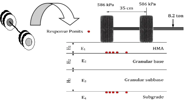
Figure 2. Specifications of standard axle, pavement section, and response points.
5. Performance of Support Vector
Machine
Statistical parameters of SVM regression for both training and testing sets are given
Application of Support Vector Machine Regression for Predicting Critical Responses …
generalization because the coefficient of determination for both training and testing set is the same.
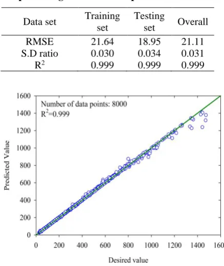
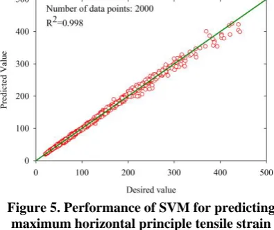
Performance of Support Vector Machine for predicting critical responses of flexible
pavement in case of training and testing sets, are presented in Figures (3) to (6). These figures confirm that the trained SVM is capable of predicting critical responses of pavement with high accuracy.
Table 1. Statistical characteristics of the inputs and outputs used in database development
Statistical Parameter H1 H2 H3 E1 E2 E3 E4 εt εc
Minimum 5.00 0.00 0.00 800.00 200.00 100.00 30.00 16.45 26.50
Maximum 45.00 50.00 60.00 10000.00 400.00 200.00 200.00 597.76 1473.29
Mean 22.69 25.98 32.73 5293.44 296.12 154.89 86.77 111.83 171.57
Standard Deviation 11.06 14.03 18.23 2800.68 64.18 29.50 38.73 82.11 150.13
Median 22.72 25.14 30.30 5056.67 300.00 153.06 82.35 86.54 126.13
Hi: Thickness of the ith layer in cm.
Ei: Resilient modulus of the ith layer in MPa.
εt: Maximum horizontal principal tensile strain at the bottom of asphalt layer in micro-strain.
εc: Maximum compressive strain on the top of subgrade in micro-strain
Table 2. Statistical parameters of SVM for predicting maximum tensile strain.
Data set Training set
Testing
set Overall
RMSE 3.56 17.70 6.37
S.D ratio 0.023 0.056 0.031
R2 0.999 0.998 0.999
Figure 3. Performance of SVM for predicting maximum horizontal principle tensile strain
based on training set.
Table 3. Statistical parameters of SVM for predicting maximum compressive strain.
Data set Training set
Testing
set Overall
RMSE 21.64 18.95 21.11
S.D ratio 0.030 0.034 0.031
R2 0.999 0.999 0.999
Figure 4. Performance of SVM for predicting maximum compressive strain on the top of
Ali Reza Ghanizadeh
[
Figure 5. Performance of SVM for predicting maximum horizontal principle tensile strain
based on testing set.
Figure 6. Performance of SVM for predicting maximum compressive strain on the top of
subgrade based on testing set.
The frequency histograms for prediction error of critical strains using training and testing sets are presented in Figure (7) and Figure (8), respectively. As can be observed, prediction error of maximum horizontal principal tensile strain at the bottom of asphalt layer and maximum compressive strain on the top of subgrade in most cases is lower than 5 percent.
6. Validation of SVM Model using
JULEA Program
The results of analysis obtained by means of JULEA program were used to validate the proposed SVM model in this study. JULEA program is among the most powerful and accurate pavement analysis programs that uses the multi-layered elastic theory for the analysis of pavements. This program has been developed by Dr. Jacob Uzan and has been employed as the analysis core for analysing flexible pavements in Mechanistic-Empirical Pavement Design Guide (MEPDG) software [NCHRP 2004]. For
comparison of responses resulted by SVM and JULEA, eight different pavement sections were considered and the critical strains at the bottom of asphalt layer and on the top of subgrade were computed using SVM model and JULEA program. The specifications of these eight pavement sections as well as the obtained responses using SVM and JULEA program are given in Table (2). As evidence, critical responses computed using SVM model are very close to the critical responses computed using JULEA. The maximum prediction error is less than 10 percent.
7. Parametric Analysis
In order to investigate the effect of different parameters on critical responses of flexible pavements, the Cosine Amplitude Method (CAM), was employed. The express similarity relation between the target function and the input parameters is used to obtain by this method. In this method, all of data pairs are expressed in the common X-space. They would form a data array X defined as Eq. (13) [Yang and Zhang, 1997]:
x x x xn
X 1, 2, 3,...,
(9)
where xi, is a vector of the length of m and is shown in the Eq. (14).
i i i im
i x x x x
x 1, 2, 3,...,
(10)
Thus, each record of the dataset can be assumed as a point in the m-dimensional space and this point requires m-coordinates to be fully defined. Equation (15) can be used to compute the strength of the relationship between xi and xj:
m
k jk m
k ik m
k jk ik
ij
x x
x x
R
1 2
1 2
1
(11)
Application of Support Vector Machine Regression for Predicting Critical Responses …
(A) (B)
Figure 7. Error percentage of predicted strain for test data: A) Maximum horizontal principle tensile strain (HPTS) at the bottom of asphalt layer and B) Maximum compressive strain on the top of subgrade
(A) (B)
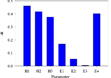
Figure 8. Error percentage of predicted strain for test data: A) Maximum horizontal principle tensile strain (HPTS) at the bottom of asphalt layer and B) Maximum compressive strain on the top of subgrade The results show that the thickness as well as
resilient modulus of asphalt concrete layer are the most influencing factors on the maximum horizontal strain at the bottom of asphalt layer. Also, the thickness of subbase layer and the resilient modulus of subgrade soil are the parameters with the least effects on the maximum horizontal strain at the bottom of asphalt layer. Moreover, thickness of different pavement layers and resilient modulus of subgrade soil are the most sensitive parameters affecting the maximum vertical strain on the top of subgrade layer, and thickness of subbase
Ali Reza Ghanizadeh
thickness lead to obvious increase in rutting life. With respect to fatigue life, it has no sensitivity with the variation of base thickness
while has a good sensitivity with the variation of surface modulus or base modulus at all values of base thickness [Behiry, 2012].
Table 4. Comparison of the responses obtained using SVM and JULEA.
H1
(cm) H2
(cm) H3
(cm) E1
(MPa) E2
(MPa) E3
(MPa) E4
(MPa)
SVM JULEA Error
percentage
εt εc εt εc εt εc
8 15 20 1500 220 110 40 377.50 939.58 383.53 861.13 -1.57 9.11
9 15 20 2000 240 120 45 320.76 760.28 320.09 717.22 0.21 6.00
10 15 20 2500 260 130 50 271.83 620.51 266.74 603.26 1.91 2.86
13 20 30 3000 280 140 55 193.46 315.49 187.13 320.59 3.38 -1.59
14 20 30 3500 300 150 60 163.09 273.85 157.79 277.49 3.36 -1.31
15 20 30 4000 320 160 65 137.26 239.12 134.30 241.80 2.20 -1.11
18 25 40 4500 340 170 70 98.45 146.12 98.23 147.54 0.22 -0.96
19 25 40 5000 360 180 75 84.15 129.18 85.08 131.30 -1.09 -1.61
εt: The maximum horizontal principal tensile strain at the bottom of asphalt layer, micro-strain
εc: The maximum compressive strain on the top of subgrade, micro-strain
Figure 9. Strength of the relationship between different parameters and maximum horizontal
strain at the bottom of asphalt layer.
Figure 10. Strength of the relationship between different parameters and maximum vertical
strain on the top of subgrade layer.
8. Conclusion
Application of Support Vector Machine Regression for Predicting Critical Responses …
spectra are commonly used for design of pavements using mechanistic-empirical methods, this research needs to be completed by developing other support vector machines in case of each loading axle.
9. References
Ahmed, M., Rahman, A., Islam, M. and Tarefder, R. (2015) “Combined effect of asphalt concrete cross-anisotropy and temperature variation on pavement stress–strain under dynamic loading”, Construction and Building Materials, Vol. 93, pp. 685-694.
AUSTROADS (2010) “Guide to Pavement Technology (APT-02/10) – Part 2: Pavement Structural Design”, Sydny, Australia: Austroads.
Behiry, A.E.A.E.M. (2012) “Fatigue and rutting lives in flexible pavement”, Ain Shams Engineering Journal, Vol. 3, Number 4, pp. 367-374.
Boussinesq, J. (1885) “Applications des potentials a l'etude de l'equilibre et du mouvement des solides elastique”, Gauthier-Villars, Paris.
Burmister, D. M., Palmer, L., Barber, E., Casagrande, A. D. and Middlebrooks, T. (1944) “The theory of stress and displacements in layered systems and applications to the design of airport runways”, Highway Research Board Proceedings, Chicago, Illinois, USA.
Duncan, J. M., Monismith, C. L. and Wilson, E. L. (1968) “Finite element analyses of pavements”, Highway Research Record, Vol. 228, pp. 18-33.
Fakhri, M. and Ghanizadeh, A. R. (2014) “Modelling of 3D response pulse at the bottom of asphalt layer using a novel function and artificial neural network”, International Journal of Pavement Engineering, Vol. 15, Number 8, pp. 671-688.
Ghanizadeh, A. R. and Ziaie, A. (2015) “NonPAS: A Program for Nonlinear Analysis of Flexible Pavements”, International Journal of Integrated Engineering, Vol. 7, Number 1, pp. 21-28.
Goktepe, A. B., Agar, E. and Lav, A. H. (2006), “Advances in backcalculating the mechanical properties of flexible pavements”, Advances in engineering software, Vol. 37, Number 7, pp. 421-431.
Gopalakrishnan, K., Agrawal, A., Ceylan, H., Kim, S. and Choudhary, A. (2013), “Knowledge discovery and data mining in pavement inverse analysis”, Transport, Vol. 28, Number 1, pp. 1-10.
Gopalakrishnan, K. and Kim, S. (2010) “Support vector machines approach to HMA stiffness
prediction. Journal of engineering mechanics”, Vol. 137, Number 2, pp. 138-146.
Harichandran, R. S., Yeh, M.-S. and Baladi, G. Y. (1990) “MICH-PAVE: A nonlinear finite element program for analysis of flexible pavements”, Transportation research record, Vol. 1286, pp. 123-131.
Hayhoe, G. F. (2002) “LEAF: A New Layered Elastic Computational Program for FAA Pavement Design and Evaluation Procedures”, Federal Aviation Administration.
Huang , Y. H. (2004) “Pavement analysis and design”, 2nd ed., USA, New Jersey: Prentice Hall, Inc.
Iran Management and Planning Organization (IMPO) (2010) “Iran Highway Asphaltic Pavements (IHAP) Code”, vol. 234, Tehran, Iran, 2nd edition.
IRC. (2012) “Guidelines for the design of flexible pavements”, 3rd ed., Indian Road Congress.
Jong, D. d., Peutz, M. and Korswagen, A. (1979) “Computer Program BISAR, Layered Systems Under Normal and Tangential Surface Loads”, Koninklijke/Shell Laboratorium, Amsterdam, Shell Research BV.
Khazanovich, L. and Wang, Q. C. (2007) “MnLayer: high-performance layered elastic analysis program”, Transportation Research Record, Vol. 2037, pp. 63-75.
Kim, M., Tutumluer, E., and Kwon, J. (2009) “Nonlinear pavement foundation modeling for three-dimensional finite-element analysis of flexible pavements”, International Journal of Geomechanics, Vol. 9, Number 5, pp. 195-208.
Lin, J. and Liu, Y. (2010) “Potholes detection based on SVM in the pavement distress image”, Paper presented at the Ninth International Symposium on Distributed Computing and Applications to Business Engineering and Science (DCABES), Hong Kong, China.
Maalouf, M., Khoury, N. and Trafalis, T. B. (2008) “Support vector regression to predict asphalt mix performance”, International journal for numerical and analytical methods in geomechanics, Vol. 32, Number 16, pp. 1989-1996.
Maher, A. and Bennert, T. A. (2008) “Evaluation of Poisson’s ratio for use in the mechanistic empirical pavement design guide (MEPDG)”, No. FHWA-NJ-2008-004.
Ali Reza Ghanizadeh
concrete pavement using structural evaluation results”, International Journal on Pavement Engineering and Asphalt Technology, Vol. 16, Number 2, pp. 21-38.
NCHRP. (2004) “Guide for mechanistic–empirical design of new and rehabilitated pavement structures”, Final Report for Project 1-37A. Washington, DC: National Cooperative Research Program.
Newmark, N. M. (1947) “Influence charts for computation of vertical displacements in elastic foundations”, Bulletin series No. 367, University of Illinois.
Odemark, N. (1949) “Investigations as to the elastic properties of soils and design of pavements according to the theory of elasticity”, Meddelande 77.
Patil, S., Mandal, S. and Hegde, A. (2012) “Genetic algorithm based support vector machine regression in predicting wave transmission of horizontally interlaced multi-layer moored floating pipe breakwater”, Advances in Engineering Software, Vol. 45, Number 1, pp. 203-212.
Raad, L., and Figueroa, J. L. (1980) “Load response of transportation support systems”, Journal of Transportation Engineering, Vol. 106, Number 1, pp. 111-128.
Sanborn, J. L., and Yoder, E. J. (1967) “Stress and displacements in an elastic mass under semiellipsoidal loads”, International Conference of Structural Design of Asphalt Pavements, USA.
Schiffman, R. L. (1962) “General analysis of stresses and displacements in layered elastic systems”, International Conference on the Structural Design of Asphalt Pavements, USA.
Smola, A. J. and Schölkopf, B. (2004) “A tutorial on support vector regression”, Statistics and computing, Vol. 14, Number 3, pp. 199-222.
Soltani, M., Moghaddam, T. B., Karim, M. R., Shamshirband, S. and Sudheer, C. (2015) “Stiffness performance of polyethylene terephthalate modified asphalt mixtures estimation using support vector machine-firefly algorithm”, Measurement, Vol. 63, pp. pp. 232-239.
Terzi, S. (2013) “Modeling for pavement roughness using the ANFIS approach”, Advances in engineering software, Vol. 57, pp. 59-64.
Uzan, J. (1994) “Advanced backcalculation techniques”, ASTM Special Technical Publication, ASTM STP, No. 1198, pp. 3–37.
Wu, J., and Cheng, E. (2010) “A novel hybrid particle swarm optimization for feature selection and kernel optimization in support vector regression”, International Conference the Computational Intelligence and Security (CIS), Nanning, China.
Xin, N., Gu, X., Wu, H., Hu, Y., and Yang, Z. (2012) “Application of genetic algorithm‐support vector regression (GA‐SVR) for quantitative analysis of herbal medicines”, Journal of Chemometrics, Vol. 26, Number 7, pp. 353-360.
Yang, Y. and Zhang, Q. (1997) “A hierarchical analysis for rock engineering using artificial neural networks”, Rock Mechanics and Rock Engineering, Vol. 30, Number 4, pp. 207-222.