Available online at http://ijdea.srbiau.ac.ir
Int. J. Data Envelopment Analysis (ISSN 2345-458X)
Vol.7, No.4, Year 2019 Article ID IJDEA-00422, 10 pages Research Article
Increasing Discrimination Efficiency in Data
Envelopment Analysis with Imprecise Input
and Output
S. Shahghobadi1*, F. Moradi2, A. Ghomashi3
(1,3)
Department of Applied Mathematics, Kermanshah Branch, Islamic Azad University, Kermanshah, Iran.
(2)
Department of Applied Mathematics, Sanandaj Branch, Islamic Azad University, Sanandaj, Iran.
Received 01 August 2019, Accepted 29 Octpber 2019
Abstract
One way to increase the discrimination ability in data envelopment analysis (DEA) is to use the pessimistic view in the performance evaluation. A traditional and usual approach to move from the optimistic to the pessimistic view is to expand the production possibility set. By expanding the production possibility set, the distance between each unit can be increased from the efficiency frontier, and then a smaller number of units are located on the boundary. On the other hand, in practical applications, we are confronted with imprecise inputs and outputs. Expressions of inputs and outputs as imprecise data can give us an opportunity to use it in order to increase the efficiency discrimination. Our view of the ambiguity in the data focus on fuzzy relation. We introduce a fuzzy monotonicity assumption and construct a fuzzy production possibility set (FPPS) with varying degrees of feasibility. Using the tolerance approach a nonsymmetric fuzzy linear programming model and subsequently a parametric DEA model are constructed. By applying this model, it will be seen that, for a specific and small tolerance of constraints, The discrimination efficiency of the units increases. Finally, we propose a procedure for ranking of DMUs and employ it to rank iranian national universities.
Keywords: Imprecise data envelopment analysis, Fuzzy relation, production possibility set ranking.
*. Corresponding author: Email: [email protected], [email protected]
60 1. Introduction
Data envelopment analysis is a mathematical programming technique which is used to compute relative efficiency, rank, return to scale, benchmarks and other applications of Decision Making Units (DMUs). It was developed by Charnes et al.[4]. The conventional DEA methods require accurate measurement of both the inputs and outputs. But in real-world problems the observed data are sometimes imprecise. However, for the first time, imprecise data envelopment analysis (IDEA) was introduced by Cooper et al.[5] and various fuzzy methods were prepared for dealing with it. A literature review on fuzzy DEA models with imprecise data can be found in [17]. Recently, Hatami-Marbini et al.[8] provided a taxonomy and a review of the fuzzy DEA methods. For more details we refer readers to it. Most of the Researches often expressed this problem with bounded intervals, fuzzy numbers and Statistical data, but our view of the ambiguity in the data focuses on fuzzy relations that have paid less attention to. We want to use imprecise data to increase the efficiency discrimination.Increasing the power of efficiency discrimination is one of the fundamental issues in data envelopment analysis.
Shen et al.[11] used both the efficiency and the inefficiency frontiers to increase the discrimination capability of DEA models. When the number of inputs and outputs is high compared to the number of units, it is essentially important to increase the discrimination capability of models to split the units into efficient and inefficient ones (see [3]). Dyson et al. [7] propose that the number of units be at least 2 × | | × | |, which attain a reliable degree of efficiency discrimination. (i) Using weight restrictions, (ii) incorporation of expert opinion and value judgements into models to obtain interactive models, (iii) providing models
based on common weights set such as cross-efficiency, (iv) and using the super-efficiency method are approaches that are often used to enhance the discrimination ability of DEA models [1,2,6,14].
S. Shahghobadi, et al. / IJDEA Vol.7, No.4, (2019), 59-68
61 levels on constraint violations. Sengupta [10] introduced fuzziness in the objective function and the constraints of the conventional DEA model but did not provide an application roadmap of his proposed framework [12]. In this study, we propose a useful practical method to pick tolerance vectors. We apply the proposed method for a case study to rank national universities of Iran. It is shown that although almost all the DMUs were efficient by classic DEA model, they rank completely by the proposed method . The rest of the paper is organized as follows: In section 2, we will have some basic ideas and definitions and section 3 contains the proposed model. Section 4 includes two examples and finally, the paper ends with a conclusion in section 5.
2. Definitions
A production plan is a specific combination of inputs and outputs such as
(x, y) where can be produced by consuming ̅ which may be possible or impossible. The set of all possible production plane called production possibility set (PPS), here it is denoted by T. Some commonly assumed properties of T are as follows:
Convexity: If (x, y) ∈T and (x′, y′) ∈T, then (x, y) + (1 − )(x′, y′) ∈T for any
∈ [0,1].
Monotonicity: If (x, y) ∈T, x′ ≥ x and
y′ ≤ y, then (x′, y′) ∈T.
Inclusion of observations: Each observed DMU (x , y ) ∈T.
Constant returns to scale (CRS): If
(x, y) ∈T, then ( x, y) ∈T for any ≥ 0.
Minimum extrapolation: T is the intersection of all sets satisfying the above assumptions.
Suppose that there are DMUs where each DMU consumes different amount of inputs to produce different amount of outputs. Let x ∈ and y ∈ show the input and output vectors
corresponding to DMU , respectively. A virtual DMU is given by (x( ), y( ))
where:
x( ) = ∑ x , Y( ) = ∑ y , ∈ S
S is a technology set. The PPS with the CRS assumption for (x , y ) is:
T = (x, y)| x ≥ x( ), y ≤ y( ), ∈ S = ∈ : ≥ 0, ∀
The CCR model for evaluating (x , y ) is as follows:
= Min
. ( x , y ) ∈ T
( -cut). Let A be a fuzzy set in X and ∈
[0, 1]. The -cut of the fuzzy set A is the crisp set A given by A = { ∈
: ( ) ≥ }.
(Binary fuzzy relation). A binary fuzzy relation (X,Y) on X× Y is defined as
(X,Y)={((x, y), (x, y)): (x, y) ∈ X × Y} where : X × Y⟶ [0, 1] is a grade of membership function. If X = Y then (X,X) is called a binary fuzzy relation on X.
3. Basics Idea and the Proposed Model In general, a production plan is possible if it dominates a virtual DMU based on a preference order i.e. (X, Y) is possible whenever provided the following constraints hold for at least one in S.
X ≥ X( ) and Y ≤ Y( ) (1)
62 constraint of by a fuzzy constraint.
(Fuzzy Monotonicity). If (x, y) ∈T,
x′ ⪰ x and y ⪰ y′, then (x′, y′) ∈T. Where ⪰ is a fuzzy relation and called “ fuzzy grater than or equal to".
(Fuzzy greater than or equal to). Let
⊆ be a set and , ∈ . The fuzzy relation ⪰ on is defined with membership function ⪰ as follows where
is the maximum acceptable tolerance, as determined by the decision maker.
⪰( , ) =
1, ≥ ;
1 + , − ≤ ≤ ;
0, ≤ − .
(2)
For ∈ [0,1], ⪰( , ) ≥ if and only if
≥ − (1 − ) . The proof of the proposition is easy and so is omitted. (Fuzzy Pareto order)[shahghobadi] Let
X = ( , , . . . , ),
Y = ( , , . . . , ) ∈ .
In Fuzzy parto preference, X ⪰ Y if and only if ⪰ for = 1,2, . . . , . If ⪰
denotes the membership function of
⪰ for = 1,2, . . . , , then (X, Y) = Min ⪰ ( , ). Based on this definition,
we proposed the fuzzy parato on the PPS input-output system:
(x, y) ⪰ (w, z) ⟺ w ⪰ x , y ⪰ z (x, y), (w, z) ∈ T.
Considering fuzzy Monotonicity with the technology set S, the PPS for (X , Y )
is: T = {(x, y)| x ⪰ x( ), y ⪯ y( ), ∈ S} Let I, O denote the indices sets of inputs and outputs, respectively.
(The degree of feasibility). We define the degree of feasibility for any (x, y) ∈ T as follows:
(x, y) =
sup ∈min{min ( , X ( )), min (Y ( ), )}
(x, y) ∈ P with the grade of membership
(x, y). Obviously, (x, y) ∈ P when the minimum value, in the above expression, will be positive at least for a ∈ S. Height [ ]=P .
Proof. First, suppose that (x, y) ∈ P and
(x, y) = 1. Regarding definition 6 there
is a ∈ S such that the constraints
x ⪰ X( ), y ⪯ Y( ) are hold precisely, i.e
X ≥ X( ), Y ≤ Y( ). Then, (X, Y) ∈ P. Conversely, suppose that (x, y) ∈ P, so there is a ̅ ∈ S where x ≥ X( ), y ≤ Y( ). Hence D( ̅) = 1, (X, Y) = 1 and finally (x, y) ∈ P .
We define P for ∈ [0,1] as follows:
P = {(X, Y)| , X ( ) ≥ , ∈ I,
(Y ( ), ) ≥ , ∈ O, } (3)
For each ∈ [0,1], P ⊆ P , where P is an −cut of .
Proof. It is a direct result of the definition 6.
Let ∈ [0,1]. If S is compact, then
P = P .
Proof. Assume that (X, Y) ∈ P . Hence,
sup ∈ D( ) ≥ . We have from
mathematical analysis that D( ) is continues. In addition, S is compact, then there is a ∗∈ S such that D( ∗) ≥ .
Regarding ??, (X, Y) ∈ P . This together Lemma complete the proof.
By selecting P , ∈ [0,1], as the PPS, the CCR model will be transformed to the following model that we call it −CCR model:
( , )( ) = min
. ( x , y ) ∈ P
∈ S
From Proposition 1 we have the following DEA model which its optimal solution is called − efficiency score.
( , )( ) = min .
∑ x − (1 − ) ≤ θx
∑ y + (1 − ) ≥ y
≥ 0
(4)
Where = ( , , . . . , ) and
= ( , , . . . , ) are the constant vectors of tolerance for inputs and outputs constraints and ∈ [0,1].
S. Shahghobadi, et al. / IJDEA Vol.7, No.4, (2019), 59-68
63 In this section, we introduce a procedure for complete ranking of all DMUs using proposed model. Our basic criteria for ranking of DMUs is only their efficiency scores. Since the efficiency score of a efficient unit is equal to 1 therefore, only inefficient DMUs are ranked. But in the proposed model when < 1 all DMUs are placed inside PPS and then scores of efficient DMUs can be distinguished from each other. For this reason the following numerical approach has been proposed: 1. Select a fixed pair appropriate vectors
(p, q).
2. Compute ( , )( ) for arbitrary values of ∈ [0,1], = 1,2, . . . , .
3. Compute the ( , ) for ∈ J, where
( , )=
∑ ( , )( )
∑ for ∈ J.
4. Rank all DMUs according to the obtained results of the Stage 3.
You can choose ≥ 0 and ≥ 0
according to the expert opinion, we propose the following approach. If denote the th input, assume that it is a stochastic variable which has normal distribution with the mean ( ) =
∑
and the standard deviation
( ) = ∑ ( ) for ∈ I. We have from stochastic?? that ( ) − 2 ( ) ≤
≤ ( ) + 2 ( ) in 95 percent of
times. So, we propose to choose such that in addition ∑ − (1 −
) ≥ ( ) − 2 ( ) for each
∈ [0,1], ∑ − (1 − ) ≥ 0. Then, we take
≤
⎩ ⎪ ⎨ ⎪
⎧max{min{ } − ( ) + 2 ( ), 0}, ( ) − 2 ( ) ≥
min{ },
( ) − 2 ( ) ≤ 0
(5)
for ∈ I. Similarity, we take
≤ max{ ( ) + 2 ( ) −
max{ }, 0} (6)
for ∈ O where ( ) =∑ and
( ) = ∑ ( ( )).
5. Numerical Example
In this section, we provide two numerical examples to illustrate advantages and application of the proposed method. As mentioned earlier, the tolerance vectors
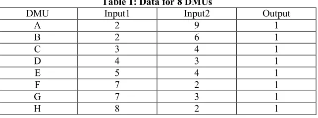
p, q could be selected according to the expert opinion. However, we select them regarding to the data dispersion according to the proposed method. A simple numerical example with 8 DMUs that consume tow inputs to produce one output is given below. The data are displayed in Table 1.
Table 1: Data for 8 DMUs
DMU Input1 Input2 Output
A 2 9 1
B 2 6 1
C 3 4 1
D 4 3 1
E 5 4 1
F 7 2 1
G 7 3 1
64 Using proposed approach for selecting tolerance vector we have ( , , ) = (2,2,0). Table 2 shows the −CCR efficiency scores for = 1,0.9,0.8,0.7,
and 0.6 . Also the ranking results of all DMUs, and are given in this table. In addition, in Table 2 we clearly see the difference between the components of each columns which leads to complete ranking of DMUs.
In this example, 33 national university in Iran were placed under investigation during 2011-2012. Each university with 9 inputs and 5 outputs in this evaluation are considered. Inputs and outputs are as follows:
Inputs: faculty member’s I , accepted students I , grade of students I , physical space per capita I , welfare
services space per capita I , The current budget for education I , scientific research I , dedicated revenue I , average rank of entrance exam I . Outputs: index of graduates O , index of papers O , index of books O , MS access pass O , the mean of passing grade O .The names of these universities are: Urmia, Isfahan, Alzahra, Boali sina, Tabriz, Tehran, Razi, Sh.Balochestan, Sh.Bahonar, Sh.Behshti, Sh.Chamran, Shiraz, Ferdosi, Gilan, Mazandaran, Yazd, Arak, Ilam, Birjand, E.Khomaini, Persion Gulf, Zabul, Zanjan, Semnan, Shahrod, Qom, Kashan, Kordestan, Lorstan, M.Ardebili, Valie asr, Hormozgan, Yasouj, respectively marked with 1 to 33. The data of these universities displayed in Table 3.
Table 3: Input and output data of 33 national university of Iran
I1 I2 I3 I4 I5 I6 I7 I8 I9 O1 O2 O3 O4 O5 DMU1 0.10 0.27 0.73 0.59 0.40 0.23 0.38 0.20 2.57 0.38 0.13 0.05 0.260.91 DMU2 0.26 0.41 0.74 0.45 0.66 0.35 0.36 0.25 4.76 0.43 0.42 0.33 0.450.90 DMU3 0.13 0.28 0.39 0.25 0.30 0.22 0.25 0.20 2.68 0.24 0.13 0.03 0.181.00 DMU4 0.12 0.30 0.54 0.68 0.37 0.22 0.44 0.18 3.82 0.26 0.12 0.13 0.260.91 DMU5 0.16 0.43 0.61 0.75 0.65 0.43 1.00 0.44 7.05 0.42 0.18 0.05 0.530.92 DMU6 1.00 1.00 0.97 0.82 0.48 1.00 0.93 1.00 18.1 1.00 1.00 1.00 1.000.93 DMU7 0.08 0.25 0.60 0.58 0.42 0.23 0.36 0.16 2.45 0.29 0.09 0.14 0.260.89 DMU8 0.07 0.43 0.98 0.22 0.62 0.40 0.38 0.21 4.24 0.24 0.04 0.05 0.220.92 DMU9 0.17 0.54 0.73 0.68 0.56 0.27 0.53 0.27 5.27 0.47 0.17 0.05 0.360.91 DMU10 0.19 0.33 0.40 0.42 0.23 0.49 0.40 0.43 5.12 0.42 0.23 0.28 0.400.95 DMU11 0.20 0.30 0.60 0.22 0.43 0.42 0.34 0.27 5.49 0.39 0.09 0.09 0.370.93 DMU12 0.20 0.40 0.54 0.89 0.63 0.59 0.47 0.37 6.70 0.44 0.69 0.05 0.490.93 DMU13 0.20 0.49 0.92 0.72 0.46 0.47 0.57 0.38 5.90 0.60 0.27 0.22 0.610.94
Table 2 :The obtained results for example 1
-efficiency -ranking
S. Shahghobadi, et al. / IJDEA Vol.7, No.4, (2019), 59-68
65
DMU14 0.16 0.19 0.41 0.48 0.51 0.21 0.41 0.20 3.42 0.34 0.08 0.09 0.310.92 DMU15 0.10 0.36 1.00 0.39 0.59 0.30 0.53 0.25 4.98 0.40 0.08 0.05 0.350.93 DMU16 0.13 0.23 0.41 1.00 0.49 0.19 0.17 0.16 2.98 0.31 0.07 0.06 0.290.93 DMU17 0.03 0.14 0.32 0.51 0.28 0.11 0.24 0.10 1.80 0.10 0.02 0.01 0.140.95 DMU18 0.04 0.14 0.31 0.21 0.39 0.11 0.23 0.08 1.70 0.04 0.01 0.02 0.050.90 DMU19 0.06 0.20 0.29 0.56 0.51 0.11 0.29 0.10 2.16 0.24 0.03 0.01 0.130.94 DMU20 0.08 0.18 0.36 0.44 0.39 0.11 0.14 0.09 4.34 0.12 0.05 0.02 0.120.91 DMU21 0.05 0.11 0.20 0.69 0.49 0.10 0.21 0.08 1.76 0.07 0.02 0.01 0.080.93 DMU22 0.11 0.27 0.85 0.21 0.23 0.16 0.11 0.15 2.45 0.32 0.01 0.01 0.090.93 DMU23 0.08 0.20 0.37 0.58 0.44 0.15 0.23 0.13 2.84 0.18 0.04 0.02 0.140.91 DMU24 0.04 0.16 0.28 0.36 0.41 0.14 0.21 0.09 3.69 0.12 0.03 0.05 0.090.90 DMU25 0.02 0.13 0.27 0.97 1.00 0.12 0.26 0.10 2.37 0.06 0.07 0.01 0.060.96 DMU26 0.07 0.14 0.25 0.55 0.53 0.08 0.17 0.08 1.89 0.09 0.01 0.04 0.060.95 DMU27 0.06 0.14 0.27 0.41 0.17 0.11 0.09 0.12 3.55 0.14 0.06 0.03 0.170.93 DMU28 0.08 0.17 0.28 0.62 0.51 0.11 0.20 0.09 2.54 0.33 0.04 0.04 0.130.88 DMU29 0.06 0.23 0.58 0.30 0.25 0.12 0.14 0.08 1.73 0.15 0.03 0.03 0.110.93 DMU30 0.06 0.19 0.32 0.61 0.63 0.09 0.20 0.07 1.88 0.28 0.05 0.06 0.100.95 DMU31 0.04 0.03 0.26 0.42 0.34 0.10 0.11 0.07 1.05 0.06 0.01 0.03 0.070.92 DMU32 0.28 0.08 0.22 0.47 0.66 0.08 0.10 0.05 1.00 0.08 0.01 0.07 0.040.95 DMU33 0.03 0.11 0.22 0.47 0.34 0.08 0.09 0.05 1.12 0.08 0.03 0.01 0.050.91
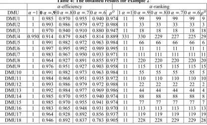
The results are computed by MATLAB software and displayed in Table 4. Using proposed approach for selecting tolerance vector we have ( , . . . , , , . . . , ) =.
(0.024, 0.028, 0.198, 0.208, 0.174, 0.079, 0.085, 0.045, 1, 0, 0, 0, 0, 0) Due to the
large number of inputs and outputs, about 89 percent of the DMUs, are efficient using by CCR model. But, all DMUs have ranked completely by the proposed procedure.
Table 4: The obtained results for example 2
-efficiency -ranking
66 2
6. Conclusion
In this study, we investigated the the classical DEA model under fuzzy
Monotonicity assumption. A parametric DEA model was obtained and used to evaluate relative efficiency of DMUs. It was seen that the obtained efficiency scores were very variety. We con conclude that if the observed units are interior points of PPS, then their efficiency scores will be dispersed, and it is important in ranking point of view. The proposed method was applied for a case study to rank national universities of Iran. It is shown that although almost all the DMUs were efficient by classic DEA model, they are completely ranked by the proposed method. How to choose the tolerance vector could be the subject for future researches.
DMU19 1 0.961 0.922 0.883 0.844 0.932 11 221 221 221 221 21 DMU20 .906 .852 .807 .764 .722 .822 32 32 32 31 31
DMU21 .932 .865 .797 .730 .882 1 29 30 30 30 0
DMU22 .974 .947 .921 .895 .954 1 16 16 16 16 6
DMU23 .803 .766 .730 .695 .660 .740 33 33 33 33 33 3
DMU24 .953 .906 .859 .812 .918 1 25 25 25 26 5
DMU25 .956 .912 .867 .823 .923 1 24 24 24 24 4
DMU26 .997 .908 .830 .759 .691 .856 30 31 31 32 32 1
DMU27 .971 .942 .913 .883 .949 1 17 17 17 17 7
DMU28 .983 .966 .949 .932 .970 1 12 12 12 12 2
DMU29 .957 .913 .870 .826 .924 1 13 13 13 13 3
DMU30 .978 .956 .935 .913 .962 1 14 14 14 14 4
DMU31 .947 .894 .842 .789 .908 1 27 27 28 28 7
DMU32 .960 .920 .880 .840 .930 1 22 22 22 22 2
S. Shahghobadi, et al. / IJDEA Vol.7, No.4, (2019), 59-68
67 References
[1] Allen, R., A. Athanassopoulos, R. G. Dyson and E. Thanassoulis (1997). "Weights restrictions and value judgements in Data Envelopment Analysis: Evolution, development and future directions." Annals of Operations Research 73(0): 13-34.
[2] Andersen, P. and N. C. Petersen (1993). "A procedure for ranking efficient units in data envelopment analysis." Management science 39(10): 1261-1264.
[3] Angulo-Meza, L. and M. P. E. Lins (2002). "Review of Methods for Increasing Discrimination in Data Envelopment Analysis." Annals of Operations Research 116(1): 225-242.
[4] Charnes A, Cooper WW, Rhodes E (1978) Measuring the efficiency of decision making units. Eur J Oper Res 2:429-444
[5] Cooper WW, Park KS, Yu G (1999) IDEA and AR-IDEA: Models for dealing with imprecise data in DEA. Manag Sci 45:597-607
[6] Doyle, J. R., R. H. Green and W. D. Cook (1995). "Upper and Lower Bound Evaluation of Multiattribute Objects: Comparison Models Using Linear Programming." Organizational Behavior and Human Decision Processes 64(3): 261-273.
[7] Dyson, R. G., R. Allen, A. S. Camanho, V. V. Podinovski, C. S. Sarrico and E. A. Shale (2001). "Pitfalls and protocols in DEA." European Journal of Operational Research 132(2): 245-259.
[8] Hatami-Marbini A, Emrouznejad A, Tavana M (2011) A taxonomy and review
of the fuzzy data envelopment analysis literature: Two decades in the making, 214:457-472
[9] Shahghobadi, S. A complete ranking of DMUs based on −efficiency in DEA with imprecise data, (2015) 8th International Conference of the Iranian Soceity of Operations Research, Ferdowsi University of Mashhad.
[10] Sengupta JK (1992) A fuzzy systems approach in data envelopment analysis. Computers and Mathematics with Applications 24(8):259-266
[11] Shen, W.-f., D.-q. Zhang, W.-b. Liu and G.-l. Yang (2016). "Increasing discrimination of DEA evaluation by utilizing distances to anti-efficient frontiers." Computers and Operations Research 75: 163-173.
[12] Sheth N, Triantis k (2003) Measuring and evaluating efficiency and effectiveness using goal programming and data envelopment analysis in a fuzzy environment, Yugoslav Journal of Operations Research 13:35-60
[13] Sexton TR, RH Silkman and AJ Hogan (1986). “Data Envelopment Analysis: Critique and Extensions.” in Silkman RH (eds.) Measuring Efficiency: An Assessment of Data Envelopment Analysis Jossey-Bass: 73-105.
[14] Thanassoulis, E., M. C. Portela and R. Allen (2004). Incorporating Value Judgments in DEA. Handbook on Data Envelopment Analysis. W. W. Cooper, L. M. Seiford and J. Zhu.Boston, MA, Springer US: 99-138.
68 Information and Decision Processes, North-Holland, Amsterdam 231-236
[16] Zimmermann HJ, Zadeh LA, Gaines AR (1984) Fuzzy Sets and Decision Analysis, North Holland, New York