Comparison of Some Data Mining Models in Forecast
of Performance of Banks Accepted in Tehran Stock
Exchange Market
Elham Adakh
PH. D Candidate, Department of Finance, faculty of Management, Islamic Azad University, Central Tehran Branch, Tehran, Iran. (Email: [email protected])
Arefeh Fadavi Asghari*
*Corresponding author, Assistant Prof., Department of Finance, Faculty of Management, Islamic Azad University, Central Tehran Branch, Tehran, Iran. (Email: [email protected])
Mohammad Ebrahim Mohammad Pourzarandi
Prof., Department of Finance, Faculty of Management, Islamic Azad University, Central Tehran Branch, Tehran, Iran. (Email: [email protected])
Abstract
In order to survive in the modern world, organizations must be equipped with the mechanisms that not only maintain their competitive advantage, but also result in their progress and improvement. Prediction of banks’ performances is an important issue, and a poor performance in banks may primarily lead to their bankruptcy, thereby affecting national economics.
The bank performance prediction model uses scientific and systematic approaches to diagnose the financial operations of institutes. According to a precise and strict evaluation, the model can detect the weakness of institutions in advance and provide early warning signals to related financial governments. In the present study, we have used three data mining models to predict the future performance of the banks accepted in Tehran Stock Exchange (TSE) and Iran Fara Bourse. Initially, 53 financial ratios were selected and, consequently, reduced to 28 using the fuzzy Delphi technique. The statistical population included 18 banks listed on TSE and Iran Fara Bourse, which provided their financial statements during the period of 2011 to 2017. Data were collected from the Codal site based on 28 financial ratios using C4.5 decision tree, AdaBoost, and Naïve Bayes algorithm. According to the findings, the Naïve Bayes algorithm was the optimal predictive model with the accuracy of 88.89%.
Keywords: Bank Performance, Data Mining, Financial Ratios, Tehran Stock Exchange.
Introduction
Performance evaluation is inherent to accountability. Various patterns and methods are available to assess the performance of companies and financial institutions; such examples are performance indicators and ratios, in which a series of variables and ratios are exploited. These variables and ratios must be identified, so that the results of the performance assessment methods could meet the needs of users, thereby leading to the continued operation of organizations and optimized use at micro and macro levels through performance improvement.
In the past, various methods have been used to assess the performance of financial institutions based on financial indicators. While the first studies in this regard primarily applied traditional statistical techniques, recent reviews have mainly used advanced decision-making approaches. Considering the growing competition in products and services, organizations need specific indicators and patterns to evaluate their performance (Porzanb et al., 2012). In the modern era, large companies and organizations are active in different regions of the world, with each operative region producing large volumes of data. Therefore, the decision-makers of corporates need access to these resources in order to make strategic decisions (Neelamadhab et al., 2012).
The banking industry undergoes constant change and development, making the recording of transaction data more convenient and causing the volume of data to grow considerably with the expansion of e-banking. The productivity of banks could enhance through the analysis of the data provided by bank databases.
Today, communities face large data storage volumes due to the increased rate of saved data. However, data use is mostly associated with the daily operations of corporates and organizations. At higher levels, managerial reports are prepared to be incorporated into decision-making processes, while attempts to search and find the available models of these data are rarely made. As such, managers must address numerous questions, which is possible if beneficial models are retrieved from the available data. For instance, managers must recognize various groups of companies that they compete with on the market. Governments seek to classify various regions across the world based on development indicators. In this regard, several methods of description and prediction could be employed to extract proper rules and models from the available data mining history.
In decision-making areas, addressing the mentioned questions requires reliance on the available data and information. Along with the opinions of experts, these data could help individuals make better decisions, and the data mining methods applied to this end are a combination of statistics, artificial intelligence, and databases (Ghazanfari et al., 2016).
The present study is aimed at assessing and comparing the efficiency of various data mining methods in predicting the performance of the banks accepted in Tehran Stock Exchange (TSE). To this end, 53 financial ratios were initially applied to evaluate the performance of the banks, and the fuzzy Delphi technique was used to reduce the ratios to 28. Afterwards, three data mining models were selected to predict the performance of the banks in the future.
Research Background
Considering that banks are the most important financial market institution in Iran, predicting their performance could increase the benefits yielded by banking operations, enhance the workplace for the employees, improve the quality of the services provided to the clients, and increase customer satisfaction. Among the other benefits of such measures are the comparison and matching of banking indicators with the global standards and development of new banking policies in the banking network of the country.
predict the performance of Islamic banks using the data of 26 Islamic banks during 1991-1993, as well as seven banking relations. In the mentioned study, the neural network was exploited to classify the banks into two categories of performance and low-performance. Among 26 banks, 12 cases were high-performance, whereas 14 cases were low-performance. In addition, the variables of liquidity and efficiency had the most significant impact on the performance of the banks (AL-Osaimy, 1995).
In another research, Odom and Sharda (1990) developed a neural network model for the prediction of bankruptcy, testing the financial data obtained from various companies, and the predictive ability of the neural network and discriminant analysis was compared. According to the findings, neural networks may be applicable to address this issue.
In another study, Becerra, Galvao, and Abou Seads (2005) proposed neural and wavelet network models to investigate financial distress, and their findings indicated that the approach was a valid alternative to the classical DA models. Moreover, wavelet networks have been shown to have numerous advantages over the conventional multilayer perceptron structures employed in neural network frameworks. Nevertheless, the feature selection problem was not investigated in the mentioned study.
On the same note, Ravi Kumar (2006) proposed an ensemble classifier using a simple majority voting scheme for the prediction of bankruptcy in banks. According to the obtained experimental results, the ensemble classifier had better performance compared to the stand-alone classifier. In another research, Sangjae and Wu Sung (2013) presented a multi-industry investigation of the bankruptcy of Korean companies using the back-propagation neural network (BNN). The studied industries included construction, retail, and manufacturing, and the findings demonstrated that the proposed model could predict bankruptcy by selecting appropriate independent variables. Furthermore, the predictive accuracy of the BNN was compared with multivariate discriminant analysis, and the results indicated that prediction using the industry samples outperformed the predictive ability of the entire samples that were not classified based on industry (6-12%). Therefore, it was reported that the predictiveaccuracy of BNN for bankruptcy was higher compared to MDA.
in TSE during 2009-2015, and the random forest algorithm was reported to be more powerful compared to the decision tree algorithm. In addition, the stock returns from the past three years and sales growth were observed to be the main variables of negative stock return prediction.
Theoretical Principles and Research Literature
The six components which played a pivotal role in the present study have been discussed in the following sub-sections.
1. Fuzzy Delphi Technique
In 1980, the fuzzy Delphi technique was introduced by Kaufman and Gupta (Chang Lin, 2002). This method is applied for decision-making and consensus on the issues where objectives and parameters are not explicit, thereby yielding highly valuable results. One of the prominent features of fuzzy Delphi technique is the provision of a flexible framework that covers several barriers associated with the lack of precision and accuracy.
Most decision-making problems are associated with incomplete and inaccurate data. Moreover, the decisions made by experts are based on their personal preferences and extremely subjective. As such, it is better to present the data in the form of fuzzy numbers rather than definitive numbers. In fact, the implementation steps of the fuzzy Delphi technique are a combination of the implementation of the Delphi method and data analyses based on the definitions of the theory of fuzzy sets. The algorithm used for the implementation of the fuzzy Delphi technique is depicted in Figure 1.
NO
YES Selecting experts and explaining the issue to them
Preparing the questionnaire and sending it to the experts
Receiving and analyzing the opinions of experts (fuzzy calculations)
Has the consensus been done properly?
The most important difference between the fuzzy Delphi and Delphi methods is that in the fuzzy Delphi technique, experts often present their ideas in the form of verbal variables, which are followed by the estimation of the mean expert opinions (numbers given), as well as the disagreement of each expert. Finally, the information is sent to experts in order to receive new ideas. At the next stage, each expert provides a new opinion based on the obtained information from the previous stage or corrects the former opinion. The process continues until the mean fuzzy number reaches sufficiently stable amount (Azar & Faraji, 2010). The qualitative variables that are defined as trapezoidal fuzzy numbers include very low (1, 1, 1, 2), low (1, 2, 3, 4), moderate (3, 4, 6, 7), high (6, 7, 8, 9), and very high (8, 9, 10, 10). Moreover, the effectiveness of each indicator on performance evaluation is estimated based on the following equations (Chang & Lin, 2002):
Am=(aim1, a m2
i , a
m3
i , a
m4
i ) = (1
n∑ a1
i,1
n∑ a2
i,1
n∑ a3
i,1
n∑ a4
i) (1)
(2)
i=1,2,3,…,n
Ai = (a1,i a2,i a3,i a4 i )
Equation 3 could be used by each of the experts to assess their opinion based on the mean opinions and modify the former opinions if desired.
E =(am1− a1i, am2− ai2, am3− a3i, am4− a4i) =
(1
n∑ a1
i − a
1
i,1
n∑ a2
i − a
2
i,1
n∑ a3
i − a
3
i,1
n∑ a4
i − a
4
i) (3)
In the present study, the differences in the opinions of the experts were determined using the equations above. In other words, the mean community at this stage and the difference between each expert of the mean community were provided to the experts in order to respond to the questions again based on the differences. At this stage, the expert was also allowed to modify or repeat their former response.
At the next stage, the differences in mean values of the first and second questionnaires were determined using the equation of the gap between the fuzzy numbers (Equation 4) in order to calculate the consensus of the experts. The fuzzy Delphi process would be discontinued if the calculated difference was less than 0.2.
S(Am1, Am2) =׀1
4[(am21+ am22+ am23+ am24) − (am11+ am12+ am13+
am14)]׀
Following that, the indicators with the mean values of less than six were eliminated (Chang & Lin, 2002).
2.Data mining and Problems Solvable with Data Mining
Data mining is the automatic discovery process of information and the identification of patterns and relationships ‘hidden’ in data.
The core process of data mining consists of building a particular model to represent the dataset that is ‘mined’ in order to solve some concrete problems of real-life. We will briefly review some of the most important issues that require the application of data mining methods, methods underlying the construction of the model.
In principle, when we use data mining methods to solve concrete problems, we have in mind their typology, which can be synthetically summarized in two broad categories, already referred to as the objectives of data mining:
Predictive methods which use some existing variables to predict future values (unknown yet) of other variables (e.g., classification, regression, etc.)
Descriptive methods that reveal patterns in data, easily interpreted by the user (e.g., clustering, association rules, sequential patterns, etc.).(Gorunescu,2011)
Prediction has been divided into two categories of regression and classification, as follows:
Regression: In this type of prediction, the variable to be predicted was numerical.
Classification: In classification problems, the variables are used to predict one or some predefined categories (Yes/No). (Ghazanfari et al., 2016).
3.Classification
Class -the dependent variable of the model- which is a categorical variable representing the ‘label’ put on the object after its classification.
Predictors -the independent variables of the model- represented by the characteristics (attributes) of the data to be classified and based on which classification is made.
Testing dataset, containing new data that will be classified by the (classifier) model constructed above, and the classification accuracy (model performance) can be evaluated.
Predictive accuracy, referring to the model’s ability to correctly classify every new, unknown object. (Gorunescu,2011)
4. C4.5 Decision Tree
A decision tree is a method used to classify data into separate categories based on a tree structure. The main goal of this technique is to find the structural information existing in the data. A decision tree is a conventional methodology applied in data mining, which simultaneously carries out regression and prediction. This technique has been widely used to resolve actual issues in the world, yielding acceptable and successful results (Komaro Ravi, 2007). C4.5 is a decision tree algorithm and a generalization of the ID3 algorithm, which uses the gain ratio criterion to select a specific trait. The algorithm stops when the number of the samples is below the determined value. On the other hand, the algorithm exploits the post-pruning technique, accepting the numerical data that are similar to the former algorithms. In addition, a modified version of the method could be applied for incomplete data (Esmaeili, 2014).
5. AdaBoost Algorithm
The AdaBoost algorithm is a collective learning technique and the most popular algorithm of the family of boosting algorithms. It was developed by Freund and Schapire in 1996 to improve classification and change a weak group of classifiers into a strong classifier (Pino et al., 2007). The algorithm functions through the education of a set of learners consistently, resulting in their combination for prediction. The boosting algorithm also uses a specific part of the dataset rather than sampling.
In order to classify all the sets in the AdaBoost algorithm, equal weights are allocated to each sample during the first repetition, and the weights are re-adjusted in the following repetitions so as to fit the data. In each repetition, the samples that have been classified inaccurately in the former repetitions gain more weights compared to the samples that have been properly classified in the previous repetitions. In addition, the classification errors that have occurred in the former repetitions are corrected in the subsequent repetitions. While the loading and modeling stages in this algorithm have similar structures, the type of the decision tree algorithm must be determined inside the operator in order to use the AdaBoost algorithm.
6. Naïve Bayes Algorithm
The Naïve Bayes classifier is a classification method, which is based on the Bayes theorem. In this algorithm, the Bayes networks explain the conditional dependencies between the variables (features), and the networks are applied to combine the former knowledge of dependency between the variables with the education model data. Some of the advantages of the Bayes method are the simple use and yielding of proper results for numerous users. In the Bayes networks, nodes are variables, each with a specific set of two-by-two incompatible states, and the bow signals the dependencies of the variables on each other (Ghazanfari et al., 2016).
Research Methodology
This was an applied research in terms of the objectives and a survey in terms of data collection.
1. Research Questions
- What are the key indicators for performance prediction?
- Which data mining methods could be used to predict the performance of banks?
- Which of the proposed models is more accurate?
2. Population, Samples, and Study Period
In the present study, data has been collected using the library method and databases relating to the subject. Initially, 53 financial ratios were selected based on the literature, which decreased to 28 ratios using the fuzzy Delphi method. It is notable that the study was performed during 2011-2017.
The sample population of the study included all the banks listed in the TSE and Fara Bourse, which presented their financial statements in 2011-2017 to the market. It is notable that Shahr Bank, Ghavamin Bank, and Resalat Bank were eliminated due to lack of access to their financial statements audited in 2017.
3. Research Stages 3.1. Phase 1
1) Data collection: primary data were extracted from the databases of the
banks.
2) Data cleaning: the most important tasks in this section included the
disruption, removal of the outliers and unrelated data, and removal of data incompatibility. The better performance in these stages of the data mining process resulted in the higher the quality of the data mining outputs and algorithms.
3) Data storage: a data warehouse was used to collect the arbitrary data from
one or more sources, their conversion into topics with information groups, and saving them together with the information on time and date to better support the decision-making process.
4) Data mart: a specific set of information was maintained, which was required
by a group of users of the data warehouse.
5) Preparation of the data for indexing: the final data were used for indexing.
3.2. Phase 2
1) Collection of the performance indicators: all the performance indicators were
collected from the topic literature.
2) Recognition of the key indicators based on the opinions of the experts and
fuzzy Delphi technique: the key indicators were determined by applying the
fuzzy Delphi technique and preparation of a questionnaire to ask the opinion of the experts.
3) Matching of the indicators based on the data warehouse: the indicators were
prepared based on the information of the data warehouse. 3.3. Phase 3
1) Entering the cleared data of the banks: the cleared data were entered.
2) Scaling: scaling was applied to prevent the feature values within greater
numeric ranges from dominating those in smaller numeric ranges, as well as the numerical difficulties in the calculations.
3) Placement of the indicators: the key indicators collected from phase two
were placed (numerical values of the indicators collected from the Codal website).
4) Modeling: the data were divided into two groups of test and education. The
5) Prediction accuracy: the precision of the model was determined after modeling.
6) Assessment: the obtained results were compared with each other.
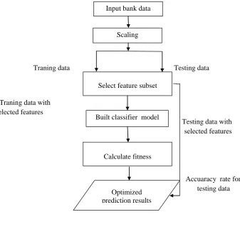
The third phase of the study is depicted in Figure 2.
Figure.2: steps of phase 3
Data Analysis
After the collection and clearing of the data, 53 financial ratios were collected from the literature of the topic and key performance evaluation ratios.
After the collection of the indicators, the ratios decreased to 28 using the fuzzy Delphi technique.
The Results of the fuzzy Delphi technique have been presented in the Table 1.
Testing data
Traning data
Traning data with
selected features
Testing data with
selected features
Accuaracy rate for testing data
Input bank data
Scaling
Select feature subset
Built classifier model
Calculate fitness
Optimized prediction results
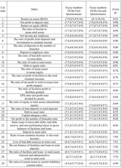
Table 1. Results of the fuzzy Delphi technique.
Col
umn Index
Fuzzy numbers Of the First Questionnaire
Fuzzy numbers Of the Second Questionnaire
Avera ge
1 Return on assets (ROA) (7/9,8/9,9/9,10) (8, 9,10,10) 9/25 2 Net profit to deposit ratio (7/7,8/7,9/7,9/9) (7/8,8/8,9/8,9/9) 9/08 3 Return on equity (ROE) (7/7,8/7,9/7,9/9) (7/7,8/7,9/7,9/9) 8/99 4 The ratio of income to mean total assets (7/7,8/7,9/7,9/9) (7/7,8/7,9/7,9/9) 8/99 5 Net Income per employee (7/6,8/6,9/6,9/8) (7/7,8/7,9/7,9/9) 8/99 6 The ratio of profits from deposits and investments to common income (7/6,8/6,9/6,9/8) (7/6,8/6,9/6,9/8) 8/90
7 The ratio of deposits to the number of branches (7/6,8/6,9/6,9/8) (7/6,8/6,9/6,9/8) 8/90 8 Deposit to employee ratio (7/6,8/6,9/6,9/8) (7/6,8/6,9/6,9/8) 8/90 9 The ratio of bad debt reserves to total debts (7/5,8/5,9/5,9/8) (7/6,8/6,9/6,9/8) 8/90 10 The ratio of cash to total assets (7/5,8/5,9/5,9/8) (7/5,8/5,9/5,9/8) 8/90 11 Debt to equity ratio (7/5,8/5,9/5,9/7) (7/6,8/6,9/6,9/8) 8/81 12 The ratio of mean assets to mean equity (7/5,8/5,9/5,9/7) (7/5,8/5,9/5,9/7) 8/78
13 The ratio of profit of facilities to the total common incomes (7/4,8/4,9/4,9/7) (7/4,8/4,9/4,9/7) 8/78
14 The ratio of net profit to total revenues (net profit margin) (7/4,8/4,9/4,9/7) (7/4,8/4,9/4,9/7) 8/73
15 The ratio of facilities profit to facilities granted (7/4,8/4,9/4,9/7) (7/5,8/5,9/5,9/7) 8/69
16 EPS ratio (net profit ratio divided by stock) (7/4,8/4,9/4,9/7) (7/4,8/4,9/4,9/7) 8/69
17 The ratio of equity to total assets (shareholder equity) (7/2,8/2,9/3,9/6) (7/4,8/4,9/4,9/7) 8/69
18 The ratio of time deposits to total deposits (7/2,8/2,9/2,9/6) (7/2,8/2,9/2,9/6) 8/60 19 Debt to asset ratio (7/1,8/1,9/2,9/5) (7/1,8/1,9/2,9/5) 8/55 20 Capital adequacy ratio (7/1,8/1,9/2,9/5) (7/3,8/3,9/3,9/6) 8/55 21 Net profit to the number of branches ratio (7/1,8/1,9/2,9/5) (7/1,8/1,9/2,9/5) 8/48
22 reserve, and non-performing loans) to gross Ratio (sum of receivable debts, bad debt balances of facilities and loans
(7/1,8/1,9/1,9/5) (7/1,8/1,9/1,9/5) 8/44
23 Deposit to asset ratio (7/1,8/1,9/1,9/5) (7/2,8/2,9/2,9/6) 8/43 24 Ratio of non-common incomes to the total incomes (6/4,7/4,8/5,9/1) (6/5,7/5,8/6,9/2) 7/95 25 Cost of bad debt reserves to total costs (6/4,7/4,8/5,9/1) (6/4,7/4,8/5,9/1) 7/91 26 The net balance of facilities and loans to total deposits (6/4,7/4,8/5,9/1) (6/4,7/4,8/5,9/1) 7/83 27 The ratio of facilities and loans to total assets (6/3,7/3,8/5,9/1) (6/5,7/5,8/6,9/2) 7/79 28 General and administrative costs to total costs (6/3,7/3,8/5,9) (6/3,7/3,8/5,9) 7/75
30 The ratio of net profit to operating income (5/5,6/5,7/7,8/4) (5/5,6/5,7/6,8/2) 6/99
31 The ratio of non-interest income to operational income (5/5,6/5,7/7,8/4) (5/5,6/5,7/7,8/4) 6/95
32 Ratio of non-operating cost on operating income (5/4,6/4,7/7,8/3) (5/4,6/4,7/7,8/3) 6/95
33 Ratio of costs of bad debt reserves to mean loans (5/4,6/4,7/7,8/3) (5/4,6/4,7/7,8/3) 6/95
34 The ratio of current debt to equity (5/5,6/5,7/7,8/3) (5/5,6/5,7/7,8/3) 6/95 35 Equity to debt ratio (5/5,6/5,7/7,8/3) (5/4,6/4,7/5,8/1) 6/95 36 Working capital (current assets minus current debts) (5/5,6/5,7/7,8/3) (5/5,6/5,7/7,8/3) 6/95
37 Quick ratio (quick assets divided by current debts) (5/4,6/4,7/7,8/3) (5/4,6/4,7/7,8/3) 6/95 38 Fixed assets to equity ratio (5/4,6/4,7/7,8/3) (5/4,6/4,7/7,8/3) 6/91 39 The ratio of the ability to pay interest (5/5,6/5,7/6,8/2) (5/5,6/5,7/6,8/1) 6/91 40 The ratio of non-interest income to non-interest costs (5/4,6/4,7/6,8/3) (5/4,6/4,7/6,8/3) 6/90 41 The ratio of dividend per share (DPS) (5/4,6/4,7/6,8/3) (5/4,6/4,7/6,8/3) 6/90 42 The ratio of cash to current debt (5/2,6/2,7/7,8/4) (5/2,6/2,7/7,8/4) 6/86
43 The ratio of net working capital to total assets (5/2,6/2,7/7,8/4) (5/4,6/4,7/8,8/5) 6/86
44 The ratio of current assets to mean daily operating costs (5/3,6/3,7/6,8/3) (5/3,6/3,7/6,8/3) 6/83
45
The difference of ratio of interest income to mean profitable interest
assets with the ratio of interest costs to mean interest debts
(5/3,6/3,7/6,8/2) (5/3,6/3,7/6,8/2) 6/83
46 The ratio of profitable assets to total assets (5/3,6/3,7/6,8/2) (5/3,6/3,7/6,8/2) 6/83
47 The ratio of the reserve of decreased value of debts to gross balances of facilities and loans
(5/3,6/3,7/5,8/2) (5/2,6/2,7/3,8/1) 6/81
48 The difference of non-interest costs with non-interest income (5/3,6/3,7/5,8/2) (5/3,6/3,7/5,8/2) 6/74
49 The ratio of non-interest costs on (total non-interest income and net interest income)
(5/2,6/2,7/5,8/1) (5/2,6/2,7/5,8/1) 6/69
50
The ratio of (difference of interest sensitive assets to interest sensitive debts) to total
assets (4/9,5/9,7/4,8/2) (5,6,7/5, 8/3) 6/69 51 The ratio of core deposits to total debts (4/7,5/7,7,7/6) (4/7,5/7,7,7/6) 6/24
52 assets to interest sensitive debts The ratio of interest sensitive (4/6,5/6,6/9,7/6) (4/6,5/6,6/9,7/6) 6/15
The difference in the mean value was not more than 0.2 after the estimation, which demonstrated the proper consensus of the experts. Based on the achieved consensus, the indicators with mean values lower than six were eliminated, and 28 indicators remained in the study.
Phase three initiated after selecting the indicators and performing the modeling process after the clearing and integration of the data. In the current research, we applied three algorithm models (C4.5 decision tree, Naïve Bayes classifier, and AdaBoost) and compared their results. In all the models, the data of the period 2011-2016 were selected as the educational data, while the data of 2017 were considered as the test data. Furthermore, the accuracy index was obtained based on the confusion matrix of each model.
In order to define the goal field, the performance of the banks in each year was divided into three categories of acceptable, moderate, and unacceptable in all the executive models of the research. The classification was based on the standards of the financial index of the central bank and opinions of six banking experts, who met the following criteria:
1. Employment as the financial manager of one of the banks listed in the TSE; 2. Minimum work experience of 20 years;
3. Minimum academic degree of MSc in financial management; 4. Thorough knowledge of financial statements and their analysis
Considering that 5-20 participants must be present in the Delphi method, we selected six experts in the current research. Afterwards, numbers one, two, and three were allocated to each ratio in the relevant year based on placement within the ranges of acceptable, moderate, and unacceptable. Finally, the performance of the banks was classified into three categories. It is also notable that the moderate range of the industry in the financial statements changes if the number of the years of research territory and banks change.
Table 2. C4.5 Decision Tree
Type of Bank Acceptabl Moderae Unacceptable Class precision
Acceptable 1 0 0 100%
Moderate 0 9 1 90%
Unacceptable 0 3 4 57.14%
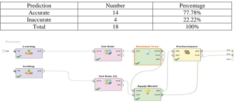
Table 3. Prediction accuracy of C4.5 Decision Tree
Prediction Number Percentage
Accurate 14 77.78%
Inaccurate 4 22.22%
Total 18 100%
Figure.3. C4.5 Decision Tree Model
Table 4. AdaBoost algorithm
Type of Bank Acceptable Moderate Unacceptable Class precision
Acceptable 1 0 0 100%
Moderate 0 10 1 90.91%
Unacceptable 0 2 4 66.67%
Table 5. Prediction accuracy of AdaBoost algorithm
Prediction Number Percentage
Accurate 15 83.33%
Inaccurate 3 16.67%
Figure.4. Adaboost Model
Table 6. Naive Bayes algorithm
Type of Bank Acceptable Moderate Unacceptable Class precision
Acceptable 1 0 0 100%
Moderate 0 11 1 91.67%
Unacceptable 0 1 4 80%
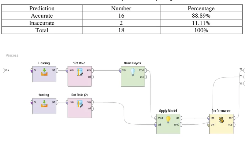
Table 7: Prediction accuracy of Naive Bayes algorithm
Prediction Number Percentage
Accurate 16 88.89%
Inaccurate 2 11.11%
Total 18 100%
Conclusion
Prediction of the performance of financial institutions is an integral principle in every organization, and this has been emphasized by the managers and stakeholders of various corporates.
Prediction is a process involving the use of a set of input variables for the estimation of the value of an output variable. Considering the contents of the current research and the fact that prediction is a major task achieved by data mining, the present study aimed to predict banking performance using data mining classification methods.
In the present study, data mining techniques were applied to predict the performance of the banks listed in Tehran Stock Exchange and Iran Fara Bourse based on their financial ratios. To this end, 53 key financial ratios were initially selected and reduced to 28 after receiving the opinions of experts and using the fuzzy Delphi technique. As a result, 28 ratios were considered as the independent variables, and the performance of the banks was determined as the dependent variable. The discretization of each ratio based on the opinions of six banking experts led to the classification of the banking performance into three levels of acceptable, moderate, and unacceptable. Furthermore, the data during the period of 2011-2016 were defined as the educational data for model construction, and the results of the model were compared to the data of 2017.
The selection of a proper method for data mining inherently depends on the nature and volume of data and data mining goals. (Esmaeili, 2014)
Based on the type of data and after the assessment of several models, we used the C4.5 decision tree, random forest, and Naïve Bayes algorithms. In total, we studied 10 banks listed on the TSE and eight banks listed on Iran Fara Bourse.
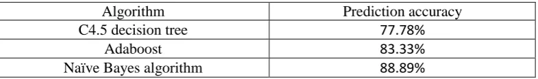
Table 8 shows the results obtained from the implementation of the three data mining models.
Table 8. Results of data mining models
Algorithm Prediction accuracy
C4.5 decision tree 77.78%
Adaboost 83.33%
As is observed, the Naïve Bayes classifier had the highest predication accuracy, followed by the AdaBoost and C4.5 decision tree algorithms, respectively. It is noteworthy that with the high accuracy of 70%, all the applied models had proper predictive power with acceptable approximation.
The accuracy of the class was 100%, which was considered acceptable in all the models. However, the accuracy of the lowest class corresponded to the unacceptable class in the C4.5 decision tree algorithm with the accuracy of 57.14%.
According to the mentioned data, the following recommendations are proposed:
The results of the present study could be beneficial for the stock market experts, and other financial institutions that are active in the field of scholarship, as well as students for future research.
References
Al-Osaimy, M. H. (1995). A Neural Networks System for Predicting Islamic Banks Performance. JKAU: Econ. & Adm., Vol. 11, p. 33-46.
Azar,A.Faraji,H,.(2010).Fuzzy management science,Mehraban publishing.(Book)
Bay vo,Bac Le,Thang N.Nguyen,.(2011).Mining frequent Itemsets from multi dimensional Data base.ACIDS '11 Proceedings of the Third international conference on Intelligent information and database systems - Volume Part I ,p. 177-186.
Becerra, V. M., Galvao, R. K. H., & Abou-Seads, M. (2005). Neural and wavelet network models for financial distress classification. Data Mining and Knowledge Discovery, 11, p.35–55.
Cheng, C. H. & Lin, Y. (2002). Evaluating the best main battle tank using fuzzy modification of Delphi. (Book)
Ehteshami, S., Hamidian, M., Hajiha, Z. and Shokrollahi,S.(2018). Forecasting Stock Trend by Data Mining Algorithm. Journal of Advances in mathematical finance & applications,3 (1),p. 97-105.
Esmaeli, Mehdi,.(2014). Concepts and techniques of data mining, Niaz Danesh publishing. (Book)
Ghazanfari,M.,Alizadeh,S., &Teimorpour,B.(2016).Data mining and knowledge discovery .(Book)
Gorunescu,F,.(2011). Concepts , Models and Techniques of data mining,Springer-Verlag Berlin Heidelberg.
Neelamadhab, P., Dr.Pragnyaban, M. and Rasmita, P.(2012). The survey of data mining applications and feature scope, International Journal of Computer Science, Engineering and Information Technology (IJCSEIT), 2(3),p.43-58.
Odom,M.D.,&Sharda,R.(1990). A neural network model for bankruptcy prediction,. Neural Networks (IJCNN), International Joint Conference on.
Pino-Mejías.R, Cubiles.M.D-de-la-Vega, Anaya-Romero.M, Pascual-Acosta.A, Jordán-López.A, and Bellinfante-Crocci.N.(2010). Predicting the potential habitat of oaks with data mining models and the R system, Journal of Environmental Modelling & Software.25(37),p.826-836.
management and of the activities of internal control in supplying usefu information through the accounting and fiscal reports, Journal of Procedia and Finance, 3, P.1099-1106.
Ravi Kumar, P., & Ravi, V. (2006). Bankruptcy prediction in banks by an ensemble classifier. In Proceedings of IEEE international conference on industrial technology, Mumbai, India.p. 2032–2036.
Ravi Kumar, P., & Ravi, V. (2007). Bankruptcy prediction in banks and firms via statistical and intelligent techniques-a review. European Journal of Operational Research, 180,p. 1–28.
Saberi, M., Rostami,M., Hamidian,M. & Aghimi,N. (2016). Forecasting the Profitability in the Firms Listed in Tehran Stock Exchange Using Data Envelopment Analysis and Artificial Neural Network.Journal of Advances in mathematical finance & applications.1 (2), p.95-104.
Sangjae,L.,& Wu Sung.C.(2013). A multi-industry bankruptcy prediction model using back-propagation neural network and multivariate discriminant analysis.International Journal of Expert systems of applications,40(8), p.2941-2946.
Bibliographic information of this paper for citing:
Adakh, Elham; Fadavi Asghari, Arefeh & Mohammad Pourzarandi, Mohammad Ebrahim (2019). Comparison of Some Data Mining Models in Forecast of Performance of Banks Accepted in Tehran Stock Exchange Market. Iranian Journal
of Finance, 3(1), 90-109.