A numerical scheme for constrained optimal control problems

Vol. 2, No. 3, pp. 233-238, July (2019)

A numerical scheme for constrained optimal

control problems

Zahra Shabani

, HalehTajadodi

1,2

Department of Mathematics, University of Sistan and Baluchestan, Zahedan, Iran

In this paper, a numerical technique is proposed to solve optimal control problems (OPCs) of Volterra integral equations (VIEs). We apply the linear B-spline polynomials to solve OPCs by VIEs. The B-spline function divides the interval into sub-intervals and then built a different approximating polynomial on each sub-interval. In this method, optimal trajectory and control functions are expanded in terms of B-spline functions. The linear B-spline operational matrix of integration and multiplication are utilized in the proposed method. The main characteristic this method is that by using the suggested numerical technique and the related operational matrices, optimal control problem governed by Volterra integral equations is converted to a system of equations. Suffice it to say that this scheme simplifies the main problems and also makes to obtain a good approximate solution for them. In the end, there are two illustrative examples which numerical results show the validity and applicability of our method.

Article Info

Keywords:

Optimal control problems, Volterra integral equations, Linear B-spline function, Operational matrix.

Article History:

Received 2018-12-26 Accepted 2019-04-15

I.

I

Optimal control theory is an important area of applied mathematics that was introduced by Pontryagin and collaborators in the 1950s.Optimal control theory has already found applications in many areas of science and engineering such as biologymedicine, economics, and finance. There are two main classes of optimal control problems (OCPs) that can be governed bydifferential equations or integral equations. Analytical and numerical methods exist for solving the various OCPs.

Therefore, recently, OCPs have been attracted attention of many researchers to obtain solutions to these problems. For more study one can see [1]-[6].There are several methods for solving differential equations[7]-[11].Among all of the techniques, orthogonal functions and polynomials have been extensively utilized for solving OCPs.Because these

polynomials and functions have high accuracy. Numerous method based on orthogonal polynomials has attempted to derive solutions of OCPsFor example,Elnagar and Razzaghi [12] in 1997s studied a pseudo spectral Legendre method for linear quadratic optimal control problems. In 2011, Maleknejad et al. [13] applied triangular functions for solving OCPs governed by VIEs.A similar argument has been obtained by Tohidi&Samadi [14].Hat functions (HFs) is used to solve linear and non-linear integral equations [15]-[16].In [17] optimal control problems including integro-differential equations is solved using Hybrid functions. In [18], Hermite wavelet is applied to solve optimal control problem. In the current paper, we suggest the linear B-spline polynomials to solve optimal control problems governed by integral equations. B-spline function is divided the interval into a collection of subintervals and construct a different approximating polynomial on each subinterval. Main applications of B-splines appear in geometric modeling, computer aided design, computer graphics and many other different subjects [19].In this scheme, the state variables and the control variables are approximated with a linear B-spline †_{Corresponding Author: [email protected]}

Tel: +98-9112839481 , University of Sistan and Baluchestan

Department of Mathematics, University of Sistan and Baluchestan, Zahedan, Iran

functions. To this end, we use Operational matrix of integration. In consequence, optimal control problems convert to systems of algebraic equations. With the result, the state variables and the control variables is obtained.

This paper is organized as follows: Section 2 contains a brief summary of linear B-spline functions on [0,1] and approximation of function. Also the operational matrix of fractional integration is computed. In Sections 3, the proposed method is used to approximate OCPs. Section 4 describes the proposed method for solving some examples. Finally, we conclude with a summary in last Section.

II.

B-S

F

O

M

O

I

A. Linear B-spline function on [0,1]

The th-order cardinal B-spline Nm(t) has the knot

sequence{⋯ , −1,0,1, ⋯ }. Also there are polynomials of order (degree − 1) between the knots. The B-spline functions for ≥ 2on [0,1]has the following form [19-23]:

= _!∑ −1 − . (1)

Where supp[ ] = [0, ]and the characteristic function for = 1 is = _{[ , ]} . The explicit presentation of

! (the linear B-spline function) is defined by De Boor et al. [19-21] as following:

! = " #2$ !

−1 −

= %2 − , ∈ [1,2, ∈ [0,1 ,

0, '()'*ℎ','., (2) Where

− = - − , ≥ ,_{0, < .} (3) Assume that _/, = _! 2/ − , 0, ∈ ℤand2_/, = 34556 /, 7 = 8(9)': : /, ≠ 0=. It is obvious that their support is:

2/, = [2 / , 2 / 2 + ], 0, ∈ ℤ. (4) In the light of these functions use on [0,1],we define

3/= : : 2/, ∩ [0,1] ≠ 0=, 0 ∈ ℤ.

It is clear that min:3_/= = −1and max:3_/= = 2/− 1, 0 ∈ ℤ. Since we need these functions on[0,1], therefore we consider: @/, = /, [ , ] , 0 ∈ ℤ. (5) Accordingly, the linear B-spline scaling functions for

= 0,1, ⋯ , 2/_{− 2 can be written by}

@/, = " #2_A$ !

B

−1 B_C2/ _{− + A D}

= E

2/ _{− ,}

!F≤ < _!F ,

2 − 2/ _{− ,}

!F ≤ < _!F!,

0, '()'*ℎ',',

(6)

The respective left and right boundary scaling functions for

= −1,2/_{− 1are:}

@/, = H1 − 2

/ _{, 0 ≤ <} !F,

0, 9. *, (7) and

@/,!F = H2

/ _{− 2}/_{+ 1, 1 −}

!F≤ < 1,

0, 9. *. (8)

B. The function approximation

For a fixed 0 = I, The expansion of J ∈ [0,1]with respect to linear B-spline functions can be approximated as: J = ∑!O 8 @K, = LMNK . (9)

WhereLand N_K are 2K+ 1vectors as:

L = [8 , 8 , ⋯ , 8!O ]M, (10) ΦK = [@ , @ , ⋯ , @!O ]M. (11) Then

LM_{= CQ J Φ}

KM R D S , (12) And symmetric matrix is given as:

S = T ΦU ΦKM R

=_!OVW

X Y Y Y Y Y

Z ! ![ 0

![ \ ![

⋱ ⋱

![

⋱

\

![ ![

!^

_ _ _ _ _ `

. (13)

C. Operational matrix of integration

In this subsection, the operational matrix of integration is obtained. Integral of vector N_K can be derived as:

Q Φa K R = bcΦK . (14)

Where b_c is 2K+ 1 × 2K+ 1 operational matrix of Integral for the linear B-spline function on[0,1] that can be obtained as follows:

bc= CQ Q Na K R NKM R D S = eS . (15) Where

e = Q Q Na K R NKM R . (16)

By using Equ. (14) and Equ. (16)

e =_!WOfW=

X Y Y Y Y Y Y Y Y

Z [ ! 1 ⋯ ⋯ 1 !

! 1

!g

! 2 ⋯ 2 1

⋱ ⋱ ⋱ ⋱ ⋮ ⋮ ⋱ ⋱ ⋱ 2 ⋮

⋱ 1 !g 1

! 1 !

! [^

_ _ _ _ _ _ _ _ `

!O !O

(17)

bc= eS . (18)

D. Product perational matrix

The product operational matrix Liof the linear B-spline function is given by

Ck_Φ

U x ΦUk x = ΦUk x Cm. (19)

Where Li is 2U+ 1 2K+ 1 matrix. For more information about operational matrix of product, refer to [24].

III.

T

P

M

This section is focused on the following class of optimal control problems by Volterra integral equations (VIEs):

I n, 4 = Q Ψ , n , 4 R , (20) subject to

n = * + Q p , q, n q , 4 q Rqa , (21) where ∈ [0,1], andΨ , n , 4 = 4! + n! + J n + r 4 where J , r are real functions in s![0,1]. Optimal control problem is determining the optimal control and the corresponding optimal state satisfying (21) while minimizing the cost function (20). To solve the problem (20)-(21), it is assumed that n , 4 , * and p , q, n q , 4 q are:

n = tM_Φ

K ,

4 = uM_Φ

K ,

w x = Wk_Φ

K , (22) p , q, n q , 4 q = ΦKk xΦK .

Where Φ_K was defined by (11) and t = [n , n , ⋯ , n!O ]M,

u = [4 , 4 , ⋯ , 4!O ]M,

y = [* , * , ⋯ , *!O ]M,

By substituting above equations in (21), we have tM_Φ

K = yMΦK +ΦKk x Q Φa K q Rq, (23)

By using operational matrix of integration and operational matrix of product, we have

tM_Φ

K = yMΦK + ΦKk xbcΦK = yMΦK +

z{M_Φ

K . (24)

Where | = x. b_c and z{ is operational matrix of product. Consequently, (24) can be expressed in term of vectors tand u which has been called Φ∗ t, u .

Now, we approximate functions J and r in Equ. (20) as:

J = ~M_Φ

K , r = •MΦK , (25)

~and• are the linear B-spline function coefficients of J and r . Substituting (22), (25) in (20), we have got: I t, u = Q Vk_Φ

K ΦKM t + uMΦK ΦKM u +

~M_Φ

K ΦKM t + •MNK NKM u R . (26)

By using (13):

I t, u = Vk_{St + u}M_{Su + ~}M_{St + •}M_{Su. (27)}

Let

I∗ _{t, u = I t, u + Φ}∗ _{t, u •. (28)}

Where • = [• , ⋯ , •_!O ] is the unknown Lagrange multiplier. The following conditions for the minimum are given by

‚I∗

‚t = 0, ‚I

∗

‚u = 0, ‚I

∗

‚• = 0.

By solving this system, the approximate values of n and 4 from Equ. (21) will be obtained.

IV.

A

Example1: Consider the following non-linear optimal control problem

I n, 4 = Q n − − 1 !_{+ 4 −} !₋ ! _{R ,}

(29) subject to

n = * + Q qa !_{4 n Rq, (30)}

where

* = −_ƒ „₋

! \−g ƒ+ + 1. (31)

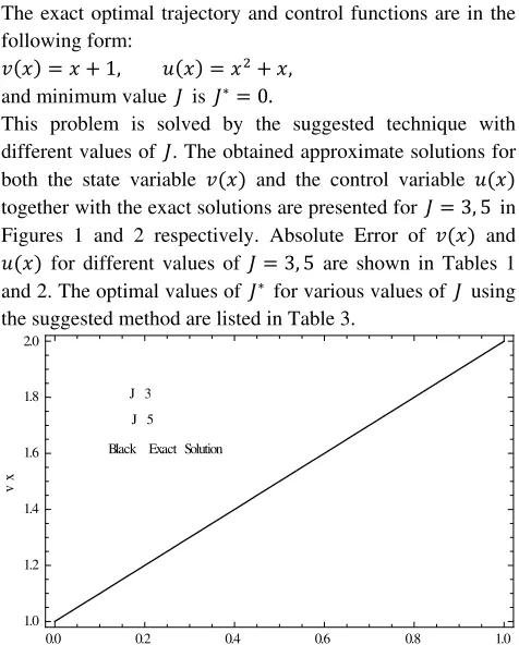
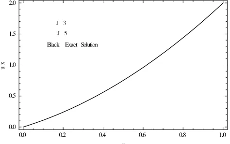
The exact optimal trajectory and control functions are in the following form:

n = + 1, 4 = !_{+ ,}

and minimum value I is I∗= 0.

This problem is solved by the suggested technique with different values of I. The obtained approximate solutions for both the state variable n and the control variable 4 together with the exact solutions are presented for I = 3, 5 in Figures 1 and 2 respectively. Absolute Error of n and 4 for different values of I = 3, 5 are shown in Tables 1 and 2. The optimal values of I∗ for various values of I using the suggested method are listed in Table 3.

Fig. 1.Exact solution and obtained approximate solution of

n for I = 3,5.

0.0 0.2 0.4 0.6 0.8 1.0

1.0 1.2 1.4 1.6 1.8 2.0

x

v

x

J 3 J 5

Fig. 2.Exact solution and obtained approximate solution of

4 for I = 3,5.

Table1. Absolute Error of n for I = 3,5 in Example 1 x J=3 J=5 0.0

0.1 0.2 0.3 0.4 0.5 0.6 0.7 0.8 0.9 1

7.78602 × 10 „

1.0498 × 10 \

2.30611 × 10 \

5.04679 × 10 \

8.37936 × 10 \

7.96199 × 10 \

2.93962 × 10 ƒ

3.40489 × 10 \

6.85843 × 10 ƒ

9.02191 × 10 ƒ

3.39718 × 10 [

6.15457 × 10 3.84529 × 10 Œ

1.0132 × 10 •

1.96066 × 10 •

3.27138 × 10 •

5.01976 × 10 •

7.34133 × 10 •

1.04666 × 10 „

1.47224 × 10 „

3.23741 × 10 „

5.54449 × 10 \

Table 2. Absolute Error of4 for I = 3,5 in Example 1 x J=3 J=5 0.0

0.1 0.2 0.3 0.4 0.5 0.6 0.7 0.8 0.9 1

2.60418 × 10 g

1.0389 × 10 [

1.14641 × 10 g

1.14681 × 10 g

1.02751 × 10 [

2.60247 × 10 g

1.00373 × 10 [

1.14903 × 10 g

1.15535 × 10 g

8.52475 × 10 ƒ

2.59003 × 10 g

1.6276 × 10 [

6.50937 × 10 \

7.16169 × 10 ƒ

7.16183 × 10 ƒ

6.50486 × 10 \

1.62752 × 10 [

6.4985 × 10 \

7.16334 × 10 ƒ

7.1646 × 10 ƒ

6.45093 × 10 \

1.62707 × 10 [

Table 3.The optimal values of I∗at different values of I for Example 1.

J I∗

3 4 5

1.36165 × 10 \

8.481 × 10 •

5.29848 × 10 Œ

Example2: Consider the following non-linear optimal control problem

I n, 4 = Q n − 'a !_{+ 4 − '}a ! _{R , (32)}

subject to

n = * + Q qa !_{4 n Rq, (33)}

where

* = 'a_{C1 − −}

!'aD + +!. (34)

For this example the exact optimal trajectory and control functions are in the following form:

n = 4 = 'a_,

and minimum value I is I∗= 0.

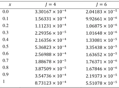
The proposed technique is applied for OCPs by VIEs with different values of I. The obtained results for the state variable n and the control variable 4 with the exact solutions for I = 4, 6 are presented in Figures 3 and 4, respectively. Absolute Error of n and 4 for different values of I = 4,6 are shown in Tables 4 and 5. The optimal values of I∗ for various values of I using the suggested method are listedin Table 6. It is apparent from the figures and tables that by increasing the value of I of B-spline basis, the approximate values of n and 4 will converge to the exact solutions.

Fig. 3.Exact solution and obtained approximate solution of

n for I = 4,6.

Fig. 4.Exact solution and obtained approximate solution of

4 for I = 4,6.

0.0 0.2 0.4 0.6 0.8 1.0

0.0 0.5 1.0 1.5 2.0

x

u

x

J 3 J 5 Black Exact Solution

0.0 0.2 0.4 0.6 0.8 1.0

1.0 1.5 2.0 2.5

x

v

x

J 4 J 6

Black Exact Solution

0.0 0.2 0.4 0.6 0.8 1.0

1.0 1.5 2.0 2.5

x

u

x

Table 4. Absolute Error of n for I = 4,6 in Example 2

I = 4 I = 6

0.0

0.1 0.2 0.3 0.4

0.5 0.6 0.7

0.8 0.9 1

3.32372 × 10 g

1.56374 × 10 [

1.12194 × 10 [

2.3081 × 10 ƒ

2.16165 × 10 [

5.37078 × 10 [

2.56637 × 10 [

1.93949 × 10 ƒ

4.01416 × 10 ƒ

3.51347 × 10 [

8.42000 × 10 [

2.04545 × 10 ƒ

9.92626 × 10 \

1.06918 × 10 \

1.01705 × 10 \

1.33074 × 10 ƒ

3.35449 × 10 ƒ

1.63637 × 10 ƒ

1.76575 × 10 \

1.68154 × 10 \

2.19326 × 10 ƒ

5.46163 × 10 ƒ

Table 5. Absolute Error of 4 for I = 4,6 in Example 2

I = 4 I = 6

0.0 0.1 0.2 0.3

0.4 0.5 0.6

0.7 0.8 0.9

1

3.30167 × 10 [

1.56331 × 10 [

1.11231 × 10 [

2.29356 × 10 ƒ

2.16356 × 10 [

5.36823 × 10 [

2.56988 × 10 [

1.88678 × 10 ƒ

3.87509 × 10 ƒ

3.54736 × 10 [

8.73123 × 10 [

2.04183 × 10 ƒ

9.92661 × 10 \

1.06875 × 10 \

1.01648 × 10 \

1.33081 × 10 ƒ

3.35438 × 10 ƒ

1.63652 × 10 ƒ

1.76371 × 10 \

1.67846 × 10 \

2.19373 × 10 ƒ

5.51078 × 10 ƒ

Table 6.The optimal values of I∗at different values of I for Example 2.

J I∗

3 4 6

2.17284 × 10 \

1.35489 × 10 „

5.28932 × 10

V.

C

This paper set out with the aim of assessing the solutions of optimal control problems by Volterra integral quations. To this end we utilized the linear B-spline polynomials. Also using the properties of operational matrices of B-spline, the cost of computational is low. The results corroborate that the proposed technique is very simple and effective.

R

[1] V. K. A. Bakke, maximum principle for an optimal control problem with integral constraints. J. Optimiz. Theory Appl., 13, 32–55, 1974.

[2] K. Maleknejad, A. Ebrahimzadeh, The use of rationalized Haar wavelet collocation method for solving optimal control of Volterra integral equations. J. Vib. Control, 21, 1958–1967, 2015.

[3] M. H. DaliriBirjandi , J. Saberi-Nadjafi , A. Ghorbani, An Efficient Numerical Method for a Class of Nonlinear VolterraIntegro-Differential Equations, Journal of Applied Mathematics, Vol. 2018, Article ID 7461058, 7 pages, doi.org/10.1155/2018/7461058.

[4] A. H., Borzabadi, A. Abbasi, O. S. Fard, Approximate optimal control for a class of nonlinear Volterra integral equations. J. Amer. Sci., 6, 1017–1021, 2010.

[5] A. Tyatyushkin and T. Zarodnyuk, Numerical method for solving optimal control problems with phase constraints,

Numerical Algebra 7, 4, 481-492, 2017.

[6] A. H. Borzabadi, M. Azizsefat, O. S. Fard, An iterative scheme for optimal control of linear Volterra integral equations. J. Adv. Res. Dyn. Control Sys., 2, 13–25, 2010. [7] D. Baleanu, H. KamilJassim and H. Khan, A modification

fractional variational iteration method for solving nonlinear gas dynamic and coupled KdV equations involving local fractional operators, Thermal Science 22, 283-283, 2018.

[8] A. Akgul, M. S. Hashemi, M. Inc, D. Baleanu and H. Khan, New method for investigating the density-dependent diffusion Nagumo equation, Thermal Science, 22, 1, 143-152, 2018.

[9] H. Khan, A. Khan, W. Chen, K. Shah, Stability analysis and a numerical scheme for fractional Klein‐Gordon

equations, Mathematical Methods in the Applied Sciences, 42, 2, 2019.

[10] M. Ahmadi Kamarposhti, Optimal Control of Islanded Micro grid Using Particle Swarm Optimization Algorithm, 1, 1, 53-60, 2018.

[11] R. Dosthosseini, N. Banisaeid and A. Dashti, Dynamic Modelling and Optimal Control of a Rotor of Active Magnetic Bearings, 2, 1, 59-70, 2019.

[12] G. N. Elnagar, M. Razzaghi, A collocation-type method for linear quadratic optimal control problems, Optim. Control Appl. Methods, 18, 227-235, 1997.

[13] K. Maleknejad, H. Almasieh, Optimal control of Volterra integral equations via triangle functions, Math. Comput. Model, 53, 1902-1909, 2011.

[14] E. Tohidi, O. R. N. Samadi, Optimal control of nonlinear Volterra integral equations via Legendre polynomials. IMA J. Math. Control Inf., 30, 67-83, 2013.

[15] E. Babolian, M. Mordad, A numerical method for solving systems of linear and nonlinear integral equations of the second kind by hat basis functions. Comput. Math. Appl., 62, 187–98, 2011.

[16] F. Mirzaee, E. Hadadiyan, Numerical solution of optimal control problem of the non-linear Volterra integral equations via generalized hat functions, IMA J. Math. Control Inf., 1-16, 2016.

[18

[19

[20

[21

[22

[23

[24

iterative methods

18] A. Kheirabadi, A. MahmoudzadehVaz

Solving optimal control problem using Hermite wavelet,

Numerical Algebra

19] C. de Boor, New York, 1978.

20] E. Cohen, R.F. Riesenfeld, and G. Elber,

Modeling with Spl

2001. 21] C.K. Chui,

Press, San Diego, 1992. 22] J.C. Goswami, and A.K. Chan,

theory, algorithms, and applications

Inc. 1999.

23] K. Sayvand, K. Pichaghchi, A novel operational matrix method for solving singularly perturbed boundary value problems of fractional multi

of Computer Mathematics

24] H. Jafari, H. Tajadodi, D. Baleanu, A numerical app for fractional order Riccati differential equation using B-spline operational matrix,

Applied Analysis

iterative methods.

A. Kheirabadi, A. MahmoudzadehVaz

Solving optimal control problem using Hermite wavelet,

Numerical Algebra, 9,1, 101

C. de Boor, A practical guide to spline

New York, 1978.

E. Cohen, R.F. Riesenfeld, and G. Elber,

Modeling with Splines: An Introduction

C.K. Chui, An introduction to wavelets

Press, San Diego, 1992. J.C. Goswami, and A.K. Chan,

theory, algorithms, and applications

d, K. Pichaghchi, A novel operational matrix method for solving singularly perturbed boundary value problems of fractional multi

of Computer Mathematics, 95, 4, 767

H. Jafari, H. Tajadodi, D. Baleanu, A numerical app for fractional order Riccati differential equation using

spline operational matrix,

Applied Analysis 18 (2), 387

Zahra Shabani

degrees from the Mashhad, Iran, respectively. Professor with

Baluchestan, Zahedan, Iran. researchinterests include

Ergodic Theory andChaos.

HalehTajadodi

degrees from the Universityof Mathematics, re

an Assistant Professor with

Sistan and Baluchestan, Zahedan, Iran. researchinterests include fractional calculus, approximation theory

.

A. Kheirabadi, A. MahmoudzadehVaziri and S. Effati, Solving optimal control problem using Hermite wavelet,

, 9,1, 101-112, 2019.

A practical guide to spline, Springer

E. Cohen, R.F. Riesenfeld, and G. Elber,

ines: An Introduction

An introduction to wavelets, Calif, Academic

J.C. Goswami, and A.K. Chan, Fundamentals of wavelets: theory, algorithms, and applications, John Wiley and Sons,

d, K. Pichaghchi, A novel operational matrix method for solving singularly perturbed boundary value problems of fractional multi-order, International Journal

, 95, 4, 767-796, 2018. H. Jafari, H. Tajadodi, D. Baleanu, A numerical app for fractional order Riccati differential equation using

spline operational matrix, Fractional Calculus and

18 (2), 387-399, 2015.

Zahra Shabani received her

from the Ferdowsi University of , Iran, all in Mathematics, She is currently an Assistant Professor with University of Sistan and Baluchestan, Zahedan, Iran. researchinterests include Dynamical Systems, Ergodic Theory andChaos.

HalehTajadodi received her from the Universityof Mathematics, respectively. Sh an Assistant Professor with

Sistan and Baluchestan, Zahedan, Iran. researchinterests include fractional calculus,

pproximation theory, optimal con iri and S. Effati, Solving optimal control problem using Hermite wavelet,

, Springer-Verlag,

E. Cohen, R.F. Riesenfeld, and G. Elber, Geometric ines: An Introduction, A.K. Peters,

, Calif, Academic

Fundamentals of wavelets:

, John Wiley and Sons,

d, K. Pichaghchi, A novel operational matrix method for solving singularly perturbed boundary value

International Journal

796, 2018.

H. Jafari, H. Tajadodi, D. Baleanu, A numerical approach for fractional order Riccati differential equation using

Fractional Calculus and

MSc and Ph.D. Ferdowsi University of all in Mathematics, e is currently an Assistant University of Sistan and Baluchestan, Zahedan, Iran. Her Dynamical Systems,

MSc and Ph.D. from the Universityof Babolsar, all in . She is currently an Assistant Professor with University of Sistan and Baluchestan, Zahedan, Iran. Her researchinterests include fractional calculus, , optimal control, iri and S. Effati, Solving optimal control problem using Hermite wavelet,

Verlag,

Geometric

, A.K. Peters,

, Calif, Academic

Fundamentals of wavelets:

, John Wiley and Sons,

d, K. Pichaghchi, A novel operational matrix method for solving singularly perturbed boundary value

International Journal

roach for fractional order Riccati differential equation using

Fractional Calculus and

Ph.D. Ferdowsi University of all in Mathematics, e is currently an Assistant University of Sistan and Her Dynamical Systems,