Hypercube Bivariate-Based Key Management for
Wireless Sensor Networks
I. Qasemzadeh Kolagar, H. Haj Seyyed Javadi
*, and M. Anzani
Department of Mathematics and Computer Sciences, Faculty of Basic Sciences, Shahed University, Tehran, Islamic Republic of Iran
Received: 1 January 2017 / Revised: 14 May 2017 / Accepted: 13 June 2017
Abstract
Wireless sensor networks are composed of very small devices, called sensor nodes,
for numerous applications in the environment. In adversarial environments, the security
becomes a crucial issue in wireless sensor networks (WSNs). There are various security
services in WSNs such as key management, authentication, and pairwise key
establishment. Due to some limitations on sensor nodes, the previous key establishment
techniques are unsuitable for WSNs. To overcome these problems, researchers propose
several key pre-distribution schemes. Our proposed approach uses a combinatorial
framework in the hypercube-based (HB) scheme to pre-distribute keys to each sensor
node. By this way, the number of common keys between two nodes in a wireless
communication range increases. Therefore, the level of security in terms of resilience
against node capture attack and the probability of re-establishing an indirect key will be
improved.
Keywords: Wireless sensor network; Key pre-distribution; Hypercube; Balanced incomplete block design (BIBD); Dynamic key path discovery algorithm.
* Corresponding author: Tel: +982151212250; Fax: +982151212201; Email: [email protected]
Introduction
A wireless sensor network (WSN) is a set of sensor nodes which have very limited storage capacity, energy and computational capabilities. WSNs have many applications such as military, smart environment, habitat monitoring, quality product monitoring, and factory process control. In such applications, since the WSN can fall susceptible to malicious attackers, security becomes an essential issue. Wireless nature of communication in WSNs, lack of infrastructure and uncontrolled environment are factors for attacking by an adversary [5]. Therefore, we are looking for a mechanism of setting up secret keys between sensor nodes. This mechanism is known the key management problem.
Three types of the key management schemes are trusted server, self-enforcing, and key pre-distribution schemes [8, 20, 22]. Since there is no fixed infrastructure in WSNs and network configuration prior to the deployment, key pre-distribution schemes (KPSs) are assumed the best solution. Many researchers propose various key pre-distribution schemes in WSNs, for example [1-3, 11, 15-17].
In the key pre-distribution schemes, a list of keys (called key-ring) is assigned to every sensor node before the deployment of the network. These keys come from the main set of all possible keys (called key pool) by a trusted key distribution center (KDC).
Eschenauer and Gligor in [12] proposed a randomized key pre-distribution scheme for sensor networks. The basic scheme is generalized by Chan et al. [7] where two nodes can communicate if they share at least 𝑞 keys in common (𝑞 > 1). Blundo et al. in [4] presented a deterministic scheme based on bivariate 𝑡-degree symmetric polynomials. Their goal was to make pairwise keys between two nodes. Liu and Ning [14] proposed a random key pre-distribution which the key pool in [12] is replaced by a pool of polynomials in [4]. In [6], Camtepe and Yener proposed a key pre-distribution scheme based on symmetric balanced incomplete design with full connectivity. However, the resilience against of node capture in these schemes is low. In this paper, considering the limitations of existing approaches, we propose an approach based on combinatorial design and hypercube-based scheme to address these issues, which we explain in the following.
Our Contributions
In this work, we propose a new deterministic key pre-distribution scheme which uses combinatorial structure in the hypercube-based (HB) scheme [14] to pre-distribute keys to each sensor node. By this way, the number of common keys between two nodes in a wireless communication range increases. Therefore, our approach improves the HB scheme in terms of resilience against node capture attack and the probability of re-establishing an indirect key, yet providing the same scalability, connectivity, and communication overhead. The idea is to generate a set of symmetric bivariate polynomials using the construction of symmetric BIBD. Each element of the blocks of symmetric BIBD is associated with each polynomial as index. Then, a list of polynomials (key-ring) is assigned to any node. In this approach, every two nodes which are at Hamming distance one from each other can establish at least one common key.
We emphasize that our main target in the proposed approach is to improve the resilience against node capture attack and the probability of re-establishing an indirect key of the HB scheme.
The remaining of the paper is arranged as follows. Section II provides the related work. In Section III, we describe our system and attack models. Section IV explains our proposed approach which uses different phases for key pre-distribution in the network. We evaluate performance and security properties of our proposed approach in section V. Section VI compares our scheme with the HB scheme. Finally, we conclude the paper in Section VII.
Related work
The key pre-distribution schemes for WSNs can use either random or deterministic approaches. In the random key pre-distribution, a random subset of keys is assigned to each sensor node from the key pool. The drawback of random scheme is that various metrics of interest in the WSN may only hold with high probability. As a result, the use of deterministic processes for selecting subsets of keys from a key pool has been proposed in various articles. Based on this classification, we show examples of random schemes and deterministic approaches.
Random Key Pre-distribution Schemes
The first random key pre-distribution scheme has been proposed by Eschenauer and Gligor [12]. This scheme is known the basic scheme. For each node, 𝑲 keys are randomly drawn out from a key pool. In this scheme, the sensor network can be regarded as a random graph in which a link exists between two nodes with a certain probability. After deployment, two neighboring nodes find a common key directly or indirectly through a secure path. Chan et al. [7] propose a modification to the basic scheme which two nodes can communicate if they share at least 𝒒 keys in common (𝒒 > 𝟏). It is shown that, by increasing the value of 𝒒,
the parameter of security increases. Liu and Ning [14] propose a random key pre-distribution which the key pool in [12] is replaced by a pool of polynomials in [4].
Deterministic Key Pre-distribution Schemes
The main foundation of random key pre-distribution schemes is the random graph theory [13]. Thus the
network layer of these schemes is random graph. Note that thenetwork layer is a graph such that two nodes are adjacent if they share a common key. The random graph cannot guarantee that any pair of neighboring nodes establishes a common key. To solve this problem, the deterministic approaches have been proposed.
Deterministic approaches can be graph-based and
grid-based schemes. In the graph-based schemes,
researchers use a complete graph or strongly regular graph. Note that a complete graph is a graph which vertices are pairwise adjacent. Some key pre-distribution schemes use the block design of combinatorial design theory in which all the nodes construct a complete graph at the network layer. For example, Camptepe and Yener [6] use balanced
incomplete block design (BIBD) in a WSN. A (𝑛2+
𝑛 + 1, 𝑛 + 1, 1)-BIBD is an arrangement into𝑛2+ 𝑛 +
what follows, we explain some properties of BIBD. A grid-based scheme is the other approach to replace the random graph. For example, Liu et al. [14] use a multi-dimensional grid which employs symmetric bivariate polynomials along each dimension. This scheme is known the hypercube-based (HB) scheme. They combine polynomial-based key pre-distribution scheme in [4] with key pool idea in [12]. This scheme arranges polynomials in a 𝑑-dimensional hypercube
[𝑚]𝑑, where 𝑚 = ⌈ √𝑁𝑑
⌉, and assigns each unique coordinate in the space as the ID to a sensor node. The setup server randomly generates 𝑑 × 𝑚𝑑−1, 𝑡-degree bivariate polynomials over a finite field 𝐹𝑝 for sufficiently large prime 𝑝. Then setup server distributes ID and polynomials to this node. To establish a pairwise key between nodes 𝑖 and 𝑗, the node 𝑖 checks the Hamming distance 𝑑ℎ between IDs of nodes 𝑖 and 𝑗. If
𝑑ℎ= 1, nodes 𝑖 and𝑗 can establish a direct key using their commonpolynomial share, otherwise they can use path discovery to establish an indirect key. Note that for an arbitrary set 𝐴, the Hamming distance between two
𝑑-tuples 𝐼, 𝐼′∈ 𝐴𝑑 is a mapping 𝑑ℎ: 𝐴𝑑× 𝐴𝑑→
{0,1, … , 𝑑} such that 𝑑ℎ(𝐼, 𝐼′) is the number of sub-indexes in which 𝐼 and 𝐼′ are different. Delgosha and Fekri [11] propose a modification to the HB scheme which uses multivariate polynomials instead of bivariate polynomials. Notice that the first polynomial-based key pre-distribution scheme has been proposed by Blundo et al. [4].
Background on BIBD
Various key pre-distribution schemes based on combinatorial design theory have been proposed by authors [6], [10], [19]. One of the tools in combinatorial design theory is BIBD. In subsection, we provide some properties of BIBD [21].
Definition 1. A set system or design is a pair (X, A), where A is a set of subsets of X, called blocks. The elements of X are the points. The degree of a point x ∈ X is the block numbers containing x. The size of the largest block is called the rank of a set system.
Definition 2. A balanced incomplete block design
(BIBD) or (v, b, r, k, λ)-BIBD is a set system with |X| = v and |A| = b such that each block of A contains exactly k elements, each element occurs in exactly r blocks, and each pair of elements occurs in exactly λ blocks of A.
In a (v, b, r, k, λ)-BIBD, we have: λ(v − 1) = r(k −
1) and bk = vr. Especial type of BIBD is called symmetric Design or symmetric BIBD denoted by
(v, k, λ)-SBIBD. In SBIBD, we have b = v and therefore r = k.
Definition 3. A finite projective plane (FPP) is a finite set of points and lines in which every pair of lines has just one intersection point and a unique line covers every pair of points.
A FPP of order q is a kind of SBIBD with parameters
(q2+ q + 1, q + 1, 1) such that every line contains exactly q + 1 points, every point occurs on exactly q +
1 lines, there are exactly q2+ q + 1 points, and there are exactly q2+ q + 1 lines in which q ≥ 2 is a prime power.
Another class of block designs is latin square with order q which is a q × q array such that each of the q symbols occurs exactly once in each column and row. Latin squares A and B of order q are orthogonal if all entries of A join B are distinct. Latin squares
A1, A2, … , Ar are mutually orthogonal latin squares (MOLS) if they are orthogonal in pairs. For prime power q, a set of (q − 1) MOLS of order q can be used to construct a finite projective plane of order q [21].
System and adversarial models System model
We consider a WSN with N sensor nodes which randomly distributed in the environment. Our scheme consists of three phases: pre-distribution, direct key establishment, and path key establishment. In the first phase, the setup server generates a finite set of 𝑡-degree bivariate symmetric polynomials and then assigns a list of it to each sensor node. After the deployment phase, any pair of neighboring nodes with the Hamming distance of one establishes a direct key using a common shared polynomial. Otherwise, the path key establishment phase takes place in which two nodes try to find a secure path for establishing an indirect key.
Adversarial model
In many scenarios, researchers investigate various types of attacks by adversaries against WSNs. For example, in [5], the authors introduce a variety of passive, active, and stealth types of attacks. An attacker can gather data from sensor nodes or can capture and read the content of them. One of the substantial attacks is node capture attack whereupon a number of randomly chosen nodes in the network is captured by an attacker. Therefore, he or she evokes all the keys or information in the nodes. Then, after capturing a certain number of nodes and removing them from the network, the secrecy of the other links between uncompromised nodes is broken. As explained in [9], an adversary may use the capture node attack as the first step for other kind of attacks. Thus, we are interested in checking the capture node attack.
The proposed approach
In this section, we present an improvement to the HB scheme [14] in terms of resilience against node capture and the probability of re-establishing an indirect key. To this end, we use a set of symmetric bivariate polynomials using the construction of symmetric BIBD. Our framework for key pre-distribution is involved in three phases: setup, direct key establishment, and path key establishment. The notations used in the present paper are illustrated in Table 1.
Setup: Given a sensor network with N nodes, we find the largest prime power q ≥ 2 such that q2+ q + 1 ≤
N. In this phase, the setup server randomly generates a set of t-degree bivariate symmetric polynomials F =
{fk(x, y)| 1 ≤ k ≤ q2+ q + 1} over a finite field Fp for sufficiently large prime power p. We consider a d
-dimensional hypercube [m]d, where m = ⌈ √Nd ⌉, in which a unique coordinate I = (i0, i1, … , id−1) is assigned to a sensor node as ID. Given a set F, the setup server constructs a symmetric BIBD with parameters
(q2+ q + 1, q + 1, 1) and associates each element of blocks with a polynomial as index. Then, the polynomials related to these q2+ q + 1 blocks are assigned to q2+ q + 1 nodes. Remaining N −
(q2+ q + 1) nodes are randomly assigned key-rings from the previous q2+ q + 1 polynomials. Therefore, any two sensor nodes can relate to the different blocks or the same block. In the different blocks and same block cases, every pair of nodes intersects in one polynomial and q + 1 polynomials, respectively. Before the deployment of the network, the setup server loads the following set to the sensor node with ID, I =
(i0, i1, … , id−1) ∈ [m]d,
FI={
fb01(i0, y), … , fbd−11 (id−1, y), … , fb0q+1(i0, y), … , fbd−1q+1(id−1, y)}.
Since every polynomial fbr(1 ≤ r ≤ q + 1) has d univariate shares of degree t, we can determine the value of t as t = ⌊M
d− 1⌋. The parameters M and dare the amount of memory required to store every polynomial share and the parameter of hypercube’s dimension, respectively. As mentioned above, we note that the setup server takes the jth position of I =
(i0, i1, … , id−1) for all 0 ≤ j ≤ d − 1 as a label for the univariate polynomials.
Example 1. Let N = 10. Then q = 2 and we construct a (7, 3, 1)-symmetric BIBD with the blocks
B = {{1, 2, 4}, {2, 3, 5}, {3, 4, 6}, {4,5,7}, {5, 6, 1}, {6, 7, 2}, {7, 1, 3}}. We can generate the polynomials related to these blocks as Bf= {{f1, f2, f4}, {f2, f3, f5},
{f3, f4, f6}, {f4, f5, f7}, {f5, f6, f1}, {f6, f7, f2}, {f7, f3, f1}}. Finally, we assign any element from Bf to seven random selected nodes out of 10 nodes. For example,
{f1, f2, f4} → node1 and {f3, f4, f6} → node2. The remaining three nodes are again assigned element from
Bf, randomly. In what follows, let d = 2. For example, for node1 with ID I1= (i0, i1) and key-ring {f1, f2, f4}, the set FI1 is equal to {f10(i0, y), f11(i1, y), f20(i0, y),
f21(i1, y), f40(i0, y), f41(i1, y)}.
Direct key establishment: After deployment, if the Hamming distance dh between two sensor nodes I and
I′ is one, then these nodes establish a direct key using a
Table 1. List of used notation
Notation Definition
𝑵 Total number of nodes in the network
𝒅𝒉(𝑰, 𝑰′) The number of subindexes in which 𝐼 = (𝑖0, 𝑖1, … , 𝑖𝑑−1) and 𝐼 = (𝑖0′, 𝑖1′, … , 𝑖𝑑−1′ ) are different
𝑰, 𝑰′∼ 𝑩
𝒊 Two nodes 𝐼 and 𝐼′ are related to the same block 𝐵𝑖
𝑰, 𝑰′≁ 𝑩
𝒊 Two nodes 𝐼 and 𝐼′ are related to different blocks 𝐵𝑖 and 𝐵𝑗; respectively.
𝒒 A power of a prime number
[m] {𝑥 ∈ 𝑍: 0 ≤ 𝑥 ≤ 𝑚 − 1}
𝒑𝒄 a fraction of compromised sensor nodes
𝑷𝒄𝒅𝒅 The probability of compromising link key between two nodes in the different blocks case
common shared polynomial. In this case, we say that these two nodes are adjacent. Assume sensor nodes I and I′ are as follows.
I = (i0, … , ij−1, ij, ij+1, … , id−1) ∈ [m]d
I′= (i
0, … , ij−1, ij′, ij+1, … , id−1) ∈ [m]d
for some j ∈ [d]. Note that dh(I, I′) = 1. Now let us establish the direct key between sensor nodes I and I′. In the different blocks case, these two nodes have one common polynomial, for example, fbk(x, y). Thus, they can establish the direct key KI,I′= fb
k j
(ij, ij′) =
fbjk(ij′, ij). In the same block case, two nodes I and I′ can establish precisely q + 1 common keys as follows.
KI,I′,k= fb k j
(ij, ij′) = fbk j
(ij′, ij), (1)
where 1 ≤ k ≤ q + 1. According to Equation (1), we can set the final common direct key KI,I′ between the nodes I and I′ as the function φ: Fpq+1→ Fp of all the
q + 1 common keys, i.e., KI,I′= φ(KI,I′,k). The function φ can be a hash function or bit-by-bit exclusive-OR function.
Path key establishment: When two sensor nodes are unable to setup a direct key, these nodes must discover at least one path to establish an indirect key. In this case, they are called nonadjacent. The discovered path contains a sequence of the intermediate nodes along the path. Note that any two consecutive intermediate nodes must have a common direct key and every node in the path must be uncompromised. Then it guarantees a secure path between any two nonadjacent sensor nodes.
If there are compromised intermediate nodes on the path or they are out of communication range, the above algorithm for finding the key path will be infeasible. To address this problem, Liu et al. [14] propose a dynamic key path discovery algorithm to find a key path between the source node and the destination node. The main idea at each step is to find a uncompromised intermediate node as a closer node to the destination node. This means that the intermediate node is closer to the destination node in terms of the Hamming distance between their IDs. The closer node has a Hamming distance of one to source node. If such intermediate node exists, then the process is repeated. If the algorithm unable to find an intermediate node closer to destination node after a few trials, then the algorithm fails. According to this algorithm, we have the two following lemmas. For proof, see [14].
Lemma 1. For any two nodes I and I′, the above
dynamic key path discovery algorithm guarantees to find a key path with dh− 1 intermediate nodes if there are no compromised nodes and any two nodes can communicate with each other, where dh is the Hamming distance between I and I′.
Lemma 2. The number of intermediate nodes in the key path discovered in the above dynamic key path discovery algorithm never exceeds 2(dh− 1).
There is an extension of the previous lemma [11].
Lemma 3. The length of the key path between the source node and the destination node discovered by the dynamic key path is at most (λ + 1)dh− λ.
In the Lemma 3, the parameter λ is a fixed positive integer and the threshold for the number of capture nodes and dh is the Hamming distance between the source node and the destination node.
Using dynamic key path discovery algorithm, we compute the probability of re-establishing an indirect key between two uncompromised nodes which will be discussed later.
Evaluation of the proposed scheme
In this section, we evaluate the performance of our proposed approach. The evaluation metrics are summarized as follows.
Scalability: As the maximum number of nodes which can be supported in a key pre-distribution scheme for a WSN [18].
Network connectivity: Probability that two neighboring nodes establish at least one common key [18].
Network resilience: Resilience against capture node usually is evaluated by computing the two probabilities: 1) probability that a random link is broken when 𝑥 nodes are captured not including in the link, and 2) when 𝑥 nodes are captured, what fraction of the communication between uncaptured nodes being captured? [18].
Storage memory: Amount of memory required to store keys in each node [5].
Communication overhead: The number of messages which sent to intermediate sensors during a key generation process [5].
Connectivity
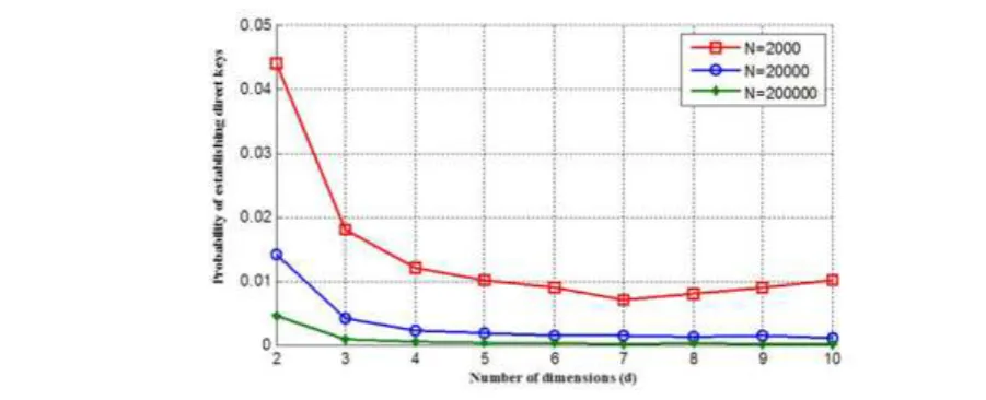
Recall that two adjacent sensor nodes can establish a direct key. Since each node in this model establishes a direct key with d(m − 1) other adjacent nodes, the probability of establishing direct keys Pdk between two adjacent nodes can be computed by d(m−1)
N−1 . Figure 1 shows the probability Pdk for the number of dimensions given different network sizes. It can be observed that by increasing the value of dimension d or N, the probability
Pdk decreases. However, for large network size N, the values of Pdk are almost same when the value of d grows.
Resilience against node capture
In this subsection, we study the security of our proposed scheme. With respect to the wireless nature of communication in a WSN, an adversary may attempt to design variety of passive and active type of attacks.
In the simplest mode of passive attacks, the adversary may capture the link between two uncompromised sensor nodes I and I′. If they are adjacent nodes, the attacker must compromise the common polynomial share of degree t between them. Assume that σ is the number of the captured nodes to compromise a direct key between two uncompromised nodes I and I′. If two nodes I and I′ are related to same block Bi, we write
I, I′∼ B
i and in the different blocks assumption, we can use I, I′≁ Bi. Therefore,
σ(t, q) = {t + 1 I, I(t + 1)(q + 1) I, I′′≁ B∼ Bi i.
Now let us compute the function for two nonadjacent nodes I and I′ in a hypercube [m]d which use the path
key establishment phase to find an indirect key. Note that even if this current key is captured by the attacker, these nodes may use different key path to establish another pairwise key. In this case, the attacker must capture all polynomial shares on one of the nodes, either
I or I′ to preventthem from establishing a new indirect key. Therefore, the function is computed by
σ(t, q, d) = {d(t + 1) I, I′∼ Bi
d(t + 1)(q + 1) I, I′≁ B i.
In the active attacks, adversaries may randomly capture sensor nodes and read the contents of them. Thus, we attend the probability of compromising a link key (direct key) and the probability of compromising any (direct or indirect) key between two uncompromised nodes under node captures.
To compute the probability of compromising a link key, we consider the link key between two uncompromised nodes in the same block case. Thus, the link key between two sensor nodes is a symmetric combination of all the q + 1 common keys between them. In order to capture a link key by the attacker, he or she must be compromised all the q + 1 common keys. We consider two nodes with IDs I =
(i0, … , ij−1, ij, ij+1, … , id−1) ∈ [m]d and I′=
(i0, … , ij−1, ij′, ij+1, … , id−1) ∈ [m]d with dh(I, I′) = 1. Let KI,I′= φ(KI,I′,k) be the final link between I and I′ where 1 ≤ k ≤ q + 1. According to Equation (1), the polynomials fb
k j (i
j, y) and fbjk(ij′, y) generate all these
q + 1 keys, where ij, ij′∈ [m]. Therefore, there exist at most m shares of fb
k j (x, y)
which is a polynomial of degree t. Thus, t + 1 shares are required to recover this
polynomial.
If m < 𝑡 + 1, there are not enough polynomial shares between two nodes to recover the corresponding common polynomial, but if m ≥ t + 1, there will be exist enough shares to recover their common polynomial.
Suppose pc is a fraction of compromised sensor nodes in the network. The probability that i shares of a particular polynomial are compromised is
P[i compromised shares] = (m
i) pci(1 − pc)m−i.
Thus, the probability of compromising a particular t -degree bivariate polynomial is
Pcd= ∑ (
m
i) pci(1 − pc)m−i.
m
i=t+1
To capture a final direct key in the same block case, all the q + 1 common keys must be captured. Then, the
probability of compromising the link key (final direct key) can be estimated by Pcds = Pcd
q+1
. Notice that the probability of compromising the link key in different blocks case is Pcdd= Pcd.
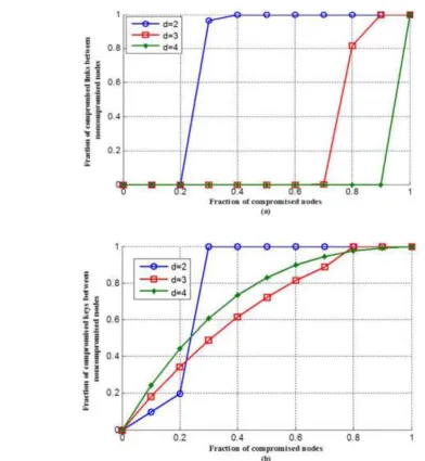
Figure 2(a) shows the probability of compromising a link key as a function of the fraction of compromised sensor nodes with different number of dimensions. We set network size N = 20000 and fixed memory constraint M = 50. We note that the probability of compromising a link key decreases when our scheme has more dimensions.
We now calculate the probability of compromising any key path between two sensor nodes I and I′ with
dh(I, I′) = i without capturing either of them. In this situation, compromising a key path will be occurred when any one of i − 1 intermediate nodes or i links on the key path is captured. Thus, the probability of compromising a key path between two sensor nodes I and I′ is
Pc= ∑ Pcd,iPi, d
i=1 where
Pi= Prob{dh(I, I′) = i} = (di) (m1) d−i
(1 −m1)i. (2)
Figure 2(b) shows by increasing the value of dimensions, the probability Pc as a function of fraction
of compromised sensor nodes decreases.
Now, we will start to study the probability of re-establishing an indirect key via dynamic key path discovery, called dynamic key. This probability is another important probability in our security analysis. Assume that S and D are the source node and the destination node, respectively, and dh(S, D) = i. Then, the shortest key path between them has length i. Let this key path be a sequence of different nodes S =
Q0, Q1, … , Qi = D such that dh(Qj−1, Qj) = 1 for 1 ≤
j ≤ i. It is mentioned that every two successive nodes
Qj−1 and Qj can be related to the same block or the different blocks. Hence, the probability of compromising the link key between them is Pcds or Pcdd. According to dynamic key path discovery algorithm, there are two ways to re-establish an indirect key between two uncompromised nodes: 1) node S finds a uncompromised intermediate node u that is closer to node D such that dh(u, D) = i − 1 and 2) if no closer node finds, then S can communicate with a uncaptured intermediate node via establishing a direct key. Then, this node discovers a closer node that is able to find a key path to node D.
Let Ii be the probability of re-establishing a dynamic key between two nodes with the Hamming distance i. The probability of discovering a closer node in the first way is
P1= [1 − ([1 − (1 − Pcds)(1 − pc)]t1
× [1 − (1 − Pcdd)(1 − pc)]i−t1)]Ii−1,
where 0 ≤ t1≤ i. In the second way, this probability can be computed by
P2= (1 − P1)[1 − ([Pcds]t2× [Pcdd]i−t2)] × [1
− ([1 − (1 − Pcds)(1 − 𝑝𝑐)]𝑡3
× [1 − (1 − 𝑃𝑐𝑑𝑑)(1 − 𝑝𝑐)]i−1−t3)]𝐼𝑖−1.
Notice that tk is the number of links on a key path between nodes which are related to the same blocks, where 1 ≤ k ≤ 3.
Thus, we have Ii= P1+ P2 for i > 1 and I1= 1 −
Pcdj , where j = 1 or q + 1. Totally, the probability of re-establishing a dynamic key is
Pre= ∑ Ii× Pi, (3) d
i=1
where Pi is defined in Equation (2).
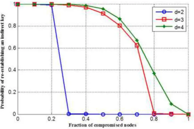
Figure 3 shows the relationship between the probability to re-establish an indirect key for uncompromised nodes and the fraction of compromised sensor nodes with different number of dimensions. In these curves, to compute Ii, we consider t1= t2=
i, t3= i − 1 and j = q + 1. It can be observed that compromising an indirect key has little effect on the probability of re-establishing a new key and there is a high probability of re-establishing another indirect key. It shows that large values of d result in higher probability of re-establishing a key.
Scalability
We consider the maximum supported network size
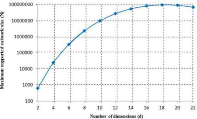
Nmaxas providing perfect resilience against the node capture. For every fixed d and t, our proposed approach derives perfect resilience when m < 𝑡 + 1. Therefore, for m = t, the maximum supported network size is
Nmax = td. Figure 4 shows that the effect of the number of dimensions on the maximum supported network size. As shown in this Figure, the maximum supported network size increases when we have more dimensions. It is worth mentioning that for dimensions close to M2, where M is the fixed memory constraint, the maximum supported network size starts to decrease. For example, in Figure 4 at dimensions d > 20, Nmax will start to drop.
Storage memory
In this subsection, we compute the overall storage memory at each sensor. The storage memory consists of amount bits to store its ID, amount bits to store the coefficients of the (q + 1)d univariate polynomials with degree t over a finite field Fp, and amount bits to store the IDs of revoked nodes. The setup server stores
(q + 1)d polynomial shares with degree t on the memory of a node I = (i0, i1, … , id−1) ∈ [m]d. Thus, it
introduces (q + 1)d(t + 1)log2|Fp|+ dlog2m bits storage space. In the other hands, to compromise a particular t -degree polynomial share, the adversary needs to capture
t + 1 shares of it. Thus, a node needs to store at most t captured node’s IDs. Since the IDs of a given node and revoked node are at the Hamming distance of one from together, then a node requires at most dtl bits storage space to store of captured node’s IDs, where l = ⌈log2m⌉.
Consequently, the overall storage memory at sensor
nodes is at most (q + 1)d(t + 1)log2|Fp|+ dl + dtl. It is clear that by increasing the value of q, storage memory at sensor node increases. To solve this problem, we can use the inequality q2+ q + 1 ≥N
2 for the smallest prime power of q instead of q2+ q + 1 ≤
N, where N is the network size. Now, we select less value for q. When qdecreases, consequently memory consumption is reduced. For example, for the network size N = 1000000, we have q = 709 instead of q =
997 which is chosen for q2+ q + 1 ≤ N. As a result, value of q decreases almost 27%. By this way, the storage memory reduces for large-scale sensor networks at the cost of reduced resilience. Therefore, depending on the applications, a network designer must establish the best trade-offs between the desired metrics.
Communication overhead
As we mentioned before, communication overhead means the number of messages which sent to intermediate sensor nodes during a secret key generation process. During the direct key establishment process, there is no communication overhead. Because this process does not involve any intermediate nodes between the source and the destination nodes.
However, during establishing an indirect key, we need to compute communication overhead. We consider a key path between the nodes I and I′ with dh(I, I′) =
i > 1. Thus, there are i − 1 intermediate nodes on this key path. Hence, the average communication in our scheme can be computed by
Cov= ∑ (i − 1)Pi= d (1 −m1) − 1 d
i=1 ,
where Pi is used in Equation (2).
Comparison
In this section, we compare our proposed approach to existing schemes.
To compare resilience against node capture between our setting and some of the existing schemes, we investigate the probabilities of compromised links and the probabilities of compromised (direct or indirect) keys versus number of compromised nodes. We consider the HB scheme with d = 2 (grid-based scheme) [14], the q-composite scheme [7], and our proposed approach. We assume that the network size and the memory constraint are fixed in all these schemes. Set N = 20000 and M = 50. In our proposed scheme, we have d = 2, q = 139, and p = 0.014. The
parameters in the grid-based scheme are m = 142 and
p = 0.014. The settings in the q-composite (q = 1) are
p = 0.014 and p = 0.33. Figure 5(a) shows that the probability of compromised links in our proposed approach always has better performance than the q -composite given p = 0.33 when the number of compromised nodes is less than about 18000 (under 90% compromised links). When the number of compromised nodes is less than 16000 (under 80% compromised links), this probability in our scheme has better performance than the q-composite given p =
0.014. When 70% of the nodes are compromised, the probabilities of compromised links in the grid-based scheme and our scheme are about 50% and zero, respectively. Similarly, Figure 5(b) shows that the probability of compromised (direct or indirect) keys in our proposed scheme performs much better than the other approaches, when the number of compromised nodes is less than about 18000 (under 90% compromised keys) in the network.
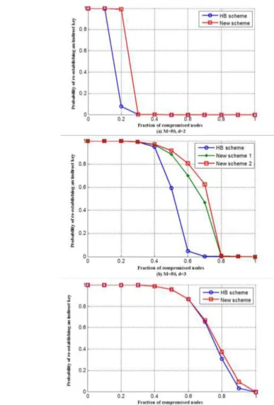
The other security metric is the probability of re-establishing an indirect key via dynamic key path discovery algorithm. Figure 6 compares this probability of our scheme with the HB scheme [14] for d = 2, d =
3, and d = 4. Other settings in these schemes are M =
50 and N = 20000. As can be seen in Figures 6(a), (b) and (c), the probability of re-establishing a dynamic key in our approach always has better performance than the HB scheme. Note that choosing the values of t1, t2 and
t3 play a significant role for value of Pre in Equation (3).
In Figure 6(a) and (c), to compute the value of Ii for 2 ≤
i ≤ d in our scheme, we set t1= t2= i and t3= i − 1. Figure 6(b) has two curves for our scheme with different values of t1, t2 and t3. In the one of them (New scheme 1), we choose t1= t2= t3= 1 and t1= t2=
t3= 2 to compute I2 and I3, respectively. It is shown that the probability of re-establishing a dynamic key in our scheme (New scheme 2) with parameters (t1=
t2= i, t3= i − 1 ) is 80% when 62% of the sensor nodes are compromised, while this probability in the New scheme 1 and the HB scheme is about 70% and zero, respectively. Note that the HB scheme and our scheme with parameters (t1= t2= i, t3= i − 1 ) have the minimum and maximum value of Pre. According to
the results, Figure 6 shows that by increasing the value of dimensions, the value of Pre is almost the same for
these schemes.
Another important factor in WSNs is the storage memory at sensor nodes. The overall storage memory at sensor nodes in our scheme becomes at most
where l = ⌈log2m⌉.
In the HB scheme [14], the overall storage memory at sensor nodes is at most
d(t + 1) (log2|Fp|+ l).
In spite of the fact that the storage memory in our scheme compared to the HB scheme is increased, the resilience against node capture and the probability of re-establishing a dynamic key are significantly enhanced. We emphasize that the communication overhead, the
Figure 5. Performance of the three key pre-distribution schemes under attacks: grid-based scheme, 𝑞-composite (𝑞 = 1), and the New scheme for M = 50, N = 20000, and d = 2. (a) Probability of compromised links versus number of compromised nodes. (b)
connectivity and the scalability in our approach are the same as the HB scheme.
Results
In this paper, we proposed an improvement to the HB scheme [14] in terms of resilience against node capture attack and the probability of re-establishing an indirect key. We illustrated that by using a combinatorial design (i.e. symmetric BIBD) in the HB scheme, we can obtain better results about security metric. Our analysis and experimental results show that the proposed scheme is more applicable for a large-scale network. Although, the storage memory in our proposed scheme is greater than the HB scheme, the resilience against node capture and the probability of re-establishing a dynamic key are significantly enhanced. For applications with a high level of security, our proposed approach is beneficial while the HB scheme is preferred for the cases with low memory usage.
Our future work would target to use the other combinatorial designs for the proposed key pre-distribution scheme and improving the other weaknesses of key pre-distribution based on hypercube, such as low resilience against some well-known attacks.
References
1. Anzani M., Haj Seyyed Javadi H. and Modiri V. Key-management scheme for wireless sensor networks based on merging blocks of symmetric design, Wirel. Netw. 1-13 (2017).
2. Anzani M., Haj Seyyed Javadi H. and Moeini A. A deterministic key pre-distribution method for wireless sensor networks based on hypercube multivariate scheme, Iran. J. Sci. Technol, A. 1-10(2016).
3. Bechkit W., Challal Y., Bouabdallah A. and Tarokh V. A Highly Scalable Key Pre-Distribution Scheme for Wireless Sensor Networks, IEEE Trans. Wireless Commun. 12(2): 948–959(2013).
4. Blundo C., Santis A.D., Herzberg A., Kutten S., Vaccaro U. and Yung M. Perfectly Secure Key Distribution for Dynamic Conferences, Information and Computation, Adv. Cryp. CRYPTO92, Springer, Santa Barbara, California, USA, 471–486(1993).
5. Camtepe S.A. and Yener B. Key distribution mechanisms for wireless sensor networks: a survey, Technical Report. Rensselaer Polytechnic Institute, Troy, New York, (2005).
6. Camtepe S.A. and Yener B. Combinatorial design of key distribution mechanisms for wireless sensor networks, IEEE/ACM Trans. Netw. 15(2): 346-358(2007).
7. Chan H., Perrig A. and Song D. Random Key pre-distribution Schemes for Sensor Networks, Proc. IEEE Sym. Security Privacy. 197-213(2003).
8. Chen C-Y. and Chao H-C. A survey of key distribution in wireless sensor networks, Secur. Commun. Netw. 7(12): 2495–2508 (2014).
9. Conti M., Pietro R.D., Mancini L.V. and Mei A. Mobility and cooperation to thwart node capture attacks in manets, EURASIP J. Wirel. Commun. Netw. 1-13(2009). 10.Dargahi T., Javadi H.H.S. and Hosseinzadeh M.
Application-specific hybrid symmetric design of key pre-distribution for wireless sensor networks, Secur. Commun. Netw. 8: 1561-1574(2015).
11.Delgosha F. and Fekri F. A multivariate key establishment scheme for wireless sensor networks, IEEE Trans. Wireless Commun. 8(4): 1814-1824(2009). 12.Eschenauer L. and Gligor V.D. A key-management
scheme for distributed sensor networks, Proc. ACM Conf. Comput. Commun. Secur. 41-47(2002).
13.Frieze A. and Karoński M. Introduction to random graphs. Cambridge University Press, (2015).
14.Liu D., Ning P. and Li R. Establishing pairwise keys in distributed sensor networks, ACM Trans. Info. Syst. Secure. 8(1): 41-77(2005).
15.Mahajan P. and Sardana A. Key distribution schemes in wireless sensor networks: novel classification and analysis, Adv. Comput. Info. Techno. 176: 43-53(2012). 16.Mitra S., Mukhopadhyay S. and Dutta R. A flexible
deterministic approach to key pre-distribution in grid based WSNs, Ad Hoc Netw. 111: 146-179(2013). 17.Modiri V., Haj Seyyed Javadi H. and Anzani M. A Novel
Scalable Key Pre-distribution Scheme for Wireless Sensor Networks based on Residual Design, Wireless Pers. Commun. (2017).
18.Pattanayak A. and Majhi B. Key pre-distribution schemes in distributed wireless sensor network using combinatorial designs revisited, Technical Report. Cryptology eprint Archive. Report 2009/131(2009). 19.Ruj S., Nayak A. and Stojmenovic I. Pairwise and triple
key distribution in wireless sensor networks with applications, IEEE Trans. Comput. 62(11): 2224-2237(2013).
20.Simplício Jr. M.A., Barreto P.S., Margi C.B. and Carvalho T.C. A survey on key management mechanisms for distributed wireless sensor networks, Comput. Netw.
54(15): 2591-2612(2010).
21.Wallis W.D. Introduction to combinatorial designs. CRC Press, (2016).