Simulating carbon exchange using a regional atmospheric model coupled to an advanced land-surface model

doi:10.5194/bg-7-2397-2010

© Author(s) 2010. CC Attribution 3.0 License.

Simulating carbon exchange using a regional atmospheric model

coupled to an advanced land-surface model

H. W. Ter Maat1, R. W. A. Hutjes1, F. Miglietta2, B. Gioli2, F. C. Bosveld3, A. T. Vermeulen4, and H. Fritsch5,* 1_{ESS-CC (Earth System Science-Climate Change), Alterra – Wageningen UR, Wageningen, The Netherlands} 2_{IBIMET, Via Giovanni Caproni 8, Florence, 50145, Italy}

3_{Royal Netherlands Meteorological Institute, De Bilt, The Netherlands}

4_{Energy Research Centre of the Netherlands (ECN), Department of Air Quality and Climate Change,} Petten, The Netherlands

5_{Max-Planck Institute for Biogeochemistry, Jena, Germany} *_{now at: Jena-Optronik, Jena, Germany}

Received: 28 July 2008 – Published in Biogeosciences Discuss.: 29 October 2008 Revised: 8 June 2010 – Accepted: 11 June 2010 – Published: 16 August 2010

Abstract. This paper is a case study to investigate what the main controlling factors are that determine atmospheric car-bon dioxide content for a region in the centre of The Nether-lands. We use the Regional Atmospheric Modelling System (RAMS), coupled with a land surface scheme simulating car-bon, heat and momentum fluxes (SWAPS-C), and including also submodels for urban and marine fluxes, which in princi-ple should include the dominant mechanisms and should be able to capture the relevant dynamics of the system. To vali-date the model, observations are used that were taken during an intensive observational campaign in central Netherlands in summer 2002. These include flux-tower observations and aircraft observations of vertical profiles and spatial fluxes of various variables.

The simulations performed with the coupled regional model (RAMS-SWAPS-C) are in good qualitative agreement with the observations. The station validation of the model demonstrates that the incoming shortwave radiation and sur-face fluxes of water and CO2are well simulated. The com-parison against aircraft data shows that the regional meteo-rology (i.e. wind, temperature) is captured well by the model. Comparing spatially explicitly simulated fluxes with aircraft observed fluxes we conclude that in general latent heat fluxes are underestimated by the model compared to the observa-tions but that the latter exhibit large variability within all flights. Sensitivity experiments demonstrate the relevance of the urban emissions of carbon dioxide for the carbon balance

Correspondence to: H. W. Ter Maat

(herbert.termaat@wur.nl)

in this particular region. The same tests also show the re-lation between uncertainties in surface fluxes and those in atmospheric concentrations.

1 Introduction

A large mismatch exists between our understanding and quantification of ecosystem atmosphere exchange of carbon dioxide at the local scale and that at the continental scale. In this paper we address some of the complexities emerging at intermediate scales.

Inverse modelling with global atmospheric tracer transport models has been used to obtain the magnitude and distribu-tion of regional CO2fluxes from variations in observed atmo-spheric CO2concentrations. However, according to Gurney et al. (2002) no consensus has yet been reached using this method and more recent “progress” in inversion modelling developments paradoxically has led to more divergent esti-mations. Gerbig et al. (2003) suggests that models require a horizontal resolution smaller than 30 km to resolve spatial variation of atmospheric CO2in the boundary layer over the continent.

2398 H. W. Ter Maat et al.: Simulating carbon exchange using a regional atmospheric model (Denning et al., 1995, 1999). Earlier studies (e.g. Bakwin et

al., 1995) showed also the importance of processes like fos-sil fuel emission and biospheric uptake on the amplitude and magnitude of diurnal and seasonal cycles of CO2 concentra-tion ([CO2]).

The hypothesis is that the uncertainties mentioned before can be reduced at the regional level if a good link between local and global scale can be established. A critical role at the regional level is played by the planetary boundary layer (PBL) dynamics influencing the transport of CO2away from the biospheric and anthropogenic sources at the sur-face. PBL processes that influence the local CO2 concen-tration are: entrainment of free tropospheric CO2 (de Arel-lano et al., 2004); subsidence; lateral advection of air con-taining CO2and convective processes leading to boundary layer growth (Culf et al., 1997). Local and global scales can be linked experimentally through a monitoring campaign of a certain region in spatial and temporal terms (Dolman et al., 2006; Gioli et al., 2004; Betts et al., 1992), preferably com-bined with model analyses using regional atmospheric trans-port models of high resolution (Perez-Landa et al., 2007a, b; Sarrat et al., 2007).

This paper will focus on modelling the regional carbon exchange of a certain region in an attempt to quantify CO2 fluxes from various sources at the surface. The following question will be addressed: What are the main controlling factors determining atmospheric carbon dioxide concentra-tion at a regional scale as a consequence of the different sur-face fluxes?

To study this regional scale interaction it is important to use land surface descriptions of appropriate complexity, that include the main controlling mechanisms and capture the rel-evant dynamics of the system, and to represent the real-world spatial variability in soils and vegetation. In this study we use a fully, online coupled model, basically consisting of the Regional Atmospheric Modelling System (RAMS; Pielke et al., 1992; Cotton et al., 2003) coupled with a land sur-face scheme carrying carbon, heat and momentum fluxes (SWAPS-C, Soil Water Atmosphere Plant System-Carbon; Ashby, 1999; Hanan et al., 1998; Hanan, 2001). Area of interest is The Netherlands where in 2002 an intensive, two week measurement campaign was held , as part of the EU-financed project RECAB (“Regional Assessment and moni-toring of the CArbo Balance within Europe”). The ensuing database has been used to calibrate and validate the models used in the present study.

First, a description of the modelling system will be given, together with the various databases (e.g. anthropogenic emis-sions) that are incorporated in the atmospheric model and how some of these databases are downscaled in time and space. A short description of the measurement campaign will also be provided, detailing the various observations taken and followed by a summary of the synoptic weather during the campaign.

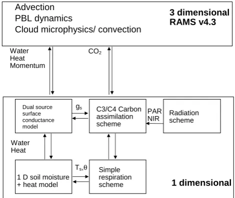
PAR

NIR Radiationscheme C3/C4 Carbon assimilation scheme Dual source surface conductance model

1 D soil moisture + heat model

Simple respiration scheme Water

Heat

Ts,θ

1 dimensional Water Heat Momentum CO2 3 dimensional RAMS v4.3 Advection PBL dynamics

Cloud microphysics/ convection

gs

Fig. 1. Schematic of the coupling between RAMS and

SWAPS-C. The main interactions between submodels is also given together

with the variables withgs– surface conductance,Ts– surface

tem-perature,θ – soil moisture, PAR – photosynthetically active

radia-tion, NIR – near infrared radiation.

Next, the results of the coupled model will be presented and compared with the observations. This paper will con-clude with a discussion of these results in terms of the factors that control the carbon dioxide content at a regional scale.

2 Description of methods/observations 2.1 Modelling system

Table 1. RAMS4.3 configuration used in this study.

Grids 1 2 3

dx, dy 48 km (83×83) 16 km (41×38) 4 km (42×42)

dt 50 s 16.7 s 16.7 s

dz 25–1000 m (35)

Radiation Harrington (1997)

Topography DEM USGS (∼1 km resolution)

Land cover PELCOM (M¨ucher et al., 2001)

Land surface SWAPS-C (Ashby, 1999; Hanan et al., 1998)

Diffusion Mellor/Yamada (Mellor and Yamada, 1982)

Convection Full microphysics package (Flatau et al., 1989)

Forcing ECMWF

Nudging time scale Lateral 1800 s

to some pre-determined large scale analysis during long model integrations. Instead a different approach was fol-lowed using the interactive nesting routine in RAMS. The smallest domain has been nested in two larger domains and the atmospheric [CO2] fields at the boundary are obtained from the parent grid (see Fig. 2). Thus, CO2 concentra-tions are free to develop, after the initial horizontal homo-geneous initialisation from (aircraft) observed concentration profiles. We assume that the spatial differences in [CO2] in the smallest domain, resulting from emissions and/or uptake at the surface, are larger than the spatial differences in back-ground [CO2] for the smallest domain. Higher [CO2], as a result of CO2-emissions originating from cities outside the smallest domain (e.g. London and major cities in the Ruhr Area in Germany), will also be fed back into the smallest do-main through the interactive nesting routine. Observations at the observatory in Mace Head at the west coast of Ireland demonstrate the small differences in background [CO2] in relative clean air masses under northern hemispheric back-ground conditions (Derwent et al., 2002). Since our analysis focuses on the smallest domain we assume that reasonable realistic horizontal gradients and associated advective fluxes develop along its edges, as a result of flux variability at the largest scales. The typical RAMS configuration used in this study is given in Table 1.

RAMS is forced by analysis data from the European Cen-tre for Medium-Range Weather Forecasts (ECMWF) global model. The grid spacing of the forcing data is 0.5 by 0.5◦

and data is available every 6 h. Monthly sea surface tem-peratures (SST) have been extracted from the Met Office Hadley Centre’s sea ice and sea surface temperature data set, HadISST1 (Rayner et al., 2003).

CO2surface fluxes come from either of three sources: – Terrestrial biospheric fluxes simulated by SWAPS-C – Marine biospheric fluxes computed from large scale

ob-served partial CO2pressures in the marine surface layer

1

2

3

Fig. 2. Configuration of the modelling domain. Boxes and numbers

illustrate the three nested grids.

– Anthropogenic CO2emissions

Each of these will be described in the following sections. 2.2 Terrestrial biospheric fluxes

Table 2. Parameters for calculating the surface conductance and the net ecosystem exchange, classified by land use. gs,max: maximum

surface conductance (mm s−1),Vm,ref: maximum catalytic capacity for Rubisco at canopy level (µmol m−2s−1) andαthe intrinsic quantum

use efficiency [−].

gs,max Vm,ref α

(mm s−1) (µmol m−2s−1) (−)

Coniferous 33.4 55.8 0.0384 Optimized

forest

Deciduous 51.0 41.0 0.0084 Ogink-Hendriks (1995),

forest Knorr (2000)

Grass 25.9 91.96 0.0283 Optimized

Agricultural 25.0 39.0 0.0475 Soet et al. (2000),

land Knorr (2000)

I

I

II

III

Fig. 3. Land cover classification (based on PELCOM) for the smallest grid in the domain. Along the flight track (black line) the location of

the observational sites are also given: C – Cabauw; W – Wageningen; H – Harskamp; L – Loobos. The roman numbers correspond to the areas described in the text.

Hanan et al. (1998) and Lloyd et al. (1995). Although these equations were originally developed for leaf scale, in SWAPS-C they are applied at canopy scale assuming the canopy can be described as a “big leaf”. Model parame-ters for each land use class were either objectively optimized against observed flux data (coniferous forest, grasslands) or taken from literature (deciduous forest and croplands, from e.g. Ogink-Hendriks, 1995; Spieksma et al., 1997; Van Wijk et al., 2000; Soet et al., 2000; Knorr, 2000; see Table 2). The parameters were optimized by minimizing the sum of squares of differences between model predictions and mea-surements using a Marquardt-Levenberg algorithm for opti-mization (Marquardt, 1963).

The land use map used in the model is extracted from the 1 km resolution PELCOM database (M¨ucher et al., 2001; Fig. 3). Soil properties were derived from the IGBP-DIS Soil

Properties database (Global Soil Data Task Group, 2000) that has a resolution of approximately 10 km (Fig. 4). In RAMS overlays are generated using vegetation and soil maps and then for each grid box the most frequently occurring soil-vegetation combinations are determined, which are then as-signed to the number of sub-grid tiles effective in that partic-ular implementation.

2.3 Marine biospheric fluxes

Fig. 4. Soil classification (depth 0–100 cm) for the smallest grid in the domain. Along the flight track (given as a black line) the location of

the observational sites are also given: C – Cabauw; W – Wageningen; H – Harskamp; L – Loobos.

month

δδδδ

pC

O

2

(µµµµ

a

tm

)

a b

Fig. 5. (a) Monthly dynamics ofδpCO2(µatm; 1 atm=1.01325 Pa) as a time series for a pixel in the North Sea (left panel), (b) Spatial

representation ofδpCO2for the Atlantic Ocean.

Hoppema (1991), who attributed this peak mainly to mix-ing of fresh water and saline North Sea water. From this seasonally varying partial pressure we derive the CO2-flux depending also on (simulated) wind speed and to a lesser de-gree on SST following Wanninkhof (1992) and Weiss (1974). To prevent unrealistic sharp flux jumps at resolutions higher than the original 5 by 4◦, we downscaled the dataset to 1◦ resolution by simple linear interpolation.

2.4 Anthropogenic CO2emissions

Anthropogenic emissions from road transport, power genera-tion and air traffic are important CO2sources in our domain. The emission inventory implemented in the RAMS/SWAPS-modelling system is the EDGAR 3.2 database (Olivier and Berdowski, 2001). The spatial resolution of this database is 1◦and annual emissions of CO2are available for 1995 (see

Fig. 6). Emissions over the oceans from shipping and upper-air emissions from upper-air traffic are neglected in this process.

To get a better spatial representation of anthropogenic emissions, these emissions are downscaled in space. This is done by equally distributing the emissions of a particu-lar 1 by 16◦grid box over all the 1 by 1 km urban pixels in the land cover map. Mismatches due to differing land-sea masks at different resolutions have been solved by distribut-ing the emission of an EDGAR pixel found over sea over its neighbouring land pixels following knowledge of the local situation.

a

b

0 0.2 0.4 0.6 0.8 1 1.2 1.4

0 50 100 150 200 250 300 350 hour

re

la

ti

v

e

fl

u

x

day of year 0

0.2 0.4 0.6 0.8 1 1.2 1.4 1.6 1.8

0 4 8 12 16 20 24

Fig. 6. (a) Anthropogenic CO2flux (terrestrial only) in µmol m−2s−1from EDGAR database version 3.2, (b) Temporal disaggregation of

these emissions: mobile emissions (left) vary diurnally, non-mobile emissions (right) vary seasonally. Note that the emission is per m2urban

area per pixel.

with no diurnal cycle. Both graphs in Fig. 6 show the relative contribution of that category to the emission. In the mobile emissions clearly a higher emission value can be seen during rush hours in the morning and evenings and almost no emis-sion during night time. The shape of this graph is based upon work done by Wickert (2001) and Kuhlwein et al. (2002). For the non-mobile emissions a different pattern can be seen with higher emissions for Europe during wintertime as a result of higher heating rates.

2.5 Region

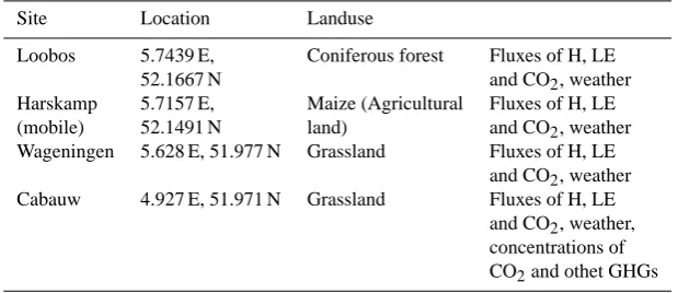
The simulations are performed for the RECAB summer cam-paign which was held between 8 and 28 July 2002. The ex-perimental region comprises a big part of the centre of The Netherlands, measuring 70 km diagonally between the flux tower of Loobos and the tall tower of Cabauw. Figures 3 and 4 both show the location of both towers together with other observational sites (Haarweg-site in Wageningen and Harskamp) which were used during the campaign. These figures also show the land use cover and the soil map of the area. On these maps four major landscape units can be dis-tinguished (Roman numbers on Fig. 3):

– hilly glacial deposits of coarse texture mainly cov-ered by various forest types (evergreen needle leaf,

deciduous broadleaf and mixed); maximum altitude 110 m a.m.s.l. (above mean sea level) (area I)

– agricultural land dominated by a mixture of grassland and maize crops on mostly sandy soils in between the hilly glacial deposits (area II)

– very low lying, wet grassland on clay and/or peat soils, mostly along the major rivers to the south of the line Wageningen – Cabauw (area III)

– urban areas (bright red areas in Fig. 3)

The region has a maritime temperate climate. During the campaign the local weather was rather unstable, cloudy and slightly colder and wetter than average. The maximum tem-perature dropped to values well below 20◦_{C at three days in}

Table 3. Description of observational sites during the RECAB campaign.

Site Location Landuse

Loobos 5.7439 E, Coniferous forest Fluxes of H, LE

52.1667 N and CO2, weather

Harskamp 5.7157 E, Maize (Agricultural Fluxes of H, LE

(mobile) 52.1491 N land) and CO₂, weather

Wageningen 5.628 E, 51.977 N Grassland Fluxes of H, LE

and CO2, weather

Cabauw 4.927 E, 51.971 N Grassland Fluxes of H, LE

and CO2, weather,

concentrations of

CO2and othet GHGs

2.6 Observations

Campaignwise observations have been made of:

– fluxes of CO2between land and atmosphere deploying permanent (3) and mobile (1) eddy-correlation flux tow-ers (see Table 3).

– aircraft fluxes of momentum, latent and sensible heat, and CO2 performed with the eddy covariance tech-nique, using a low-flying aircraft (Sky Arrow ERA). Flight altitude was 80 m a.g.l. (above ground level). The methodology and the validation of such measurements against flux towers can be found in Gioli et al. (2004). – convective boundary layer (CBL) concentrations of

CO2 and other greenhouse gases, deploying flask-and continuous sampling from an aircraft (Piper Cherokee), and continuous sampling from the tall tower at Cabauw. 2.7 Aircraft fluxes uncertainty estimation

Aircraft eddy fluxes typically show a high variability, that is related to random flux errors like those induced by large con-vective structures, spatial heterogeneity, and transient pro-cesses like mesoscale motions. To estimate such contribu-tions to observed variability and derive uncertainty figures, multiple passes over the same area in stationary conditions can be used (Mahrt et al., 2001), but such an approach is pos-sible only for small areas that can be adequately sampled in short amount of time. The experimental strategy used in RE-CAB was instead to fly and sample large areas comparable to regional model domains, with a small number of repetitions. To partially overcome this limitation in characterizing uncertainty, fluxes have been computed on a 2 km spatial length, then groups of four consecutive windows over homo-geneous landscape units have been averaged to derive 8 km fluxes, that are still comparable with model resolution. The standard deviation of such averaging process is related to random flux errors, surface heterogeneity within the 8 km

length, and non stationarity of fluxes on larger time scales. This latter effect can generally be ruled out because of the short amount of time that separates the averaged 2 km win-dows, up to few minutes. Thus an uncertainty estimation, mostly related to random flux error and surface heterogene-ity, is derived and used to interpret the observations.

Flying days during the campaign were on 15, 16, 23, 24, 25, 26 and 27 July with the last day in the best meteorological conditions. On 15, 16, 24 and 27 July two return flights from Loobos to Cabauw were performed with the low-flying eddy-correlation flux aircraft and on 15, 16 and 27 July vertical profiles were taken in the morning and in the afternoon with the aircraft performing CBL measurements. This paper will focus on the first period of the summer campaign as for these days multiple reliable observations are available to test the model.

3 Results and analyses

(a)

Incoming shortwave radiation at Loobos

Date

15-07 17-07 19-07 21-07 23-07

Sin

(W

m

-2)

-200 0 200 400 600 800 1000

(b)

Incoming shortwave radiation at Cabauw

Date

15-07 17-07 19-07 21-07 23-07

Sin

(W

m

-2)

-200 0 200 400 600 800 1000

Fig. 7. Comparison of observed and simulated incoming shortwave

radiation fluxes (W m−2) at the Loobos and Cabauw sites.

Dia-monds and dotted lines: observed values. Black lines simulated at a grid point nearest to the Loobos site and representing the appro-priate tile. Tick marks are placed at 00:00 h, same for Figs. 8, 9 and 14.

3.1 Validation against station observations

In the first set of graphs we compare simulated fluxes at grid and patch level with observed fluxes at the tower sites. Each grid box of a model can represent more than one land use class in the so-called tile-approach for sub-grid variability. We compare fluxes for the grid box nearest to the tower-site, and for the land cover class most resembling the land cover at the tower site. For the grid cell including the Loobos pine forest site we find the following distribution of land use classes 44% forest, 44% grassland and 11% agriculture. The same grid cell also covers the nearby Harskamp maize site. The grid cell containing the Cabauw grass site contains 100% grassland. The Wageningen (grassland in reality) grid

Table 4. Statistical analysis of simulated against observed

short-wave incoming radiation (W m−2), latent heat flux (W m−2) and

net ecosystem exchange (µmol m−2s−1). These statistics are

based on hourly observations and simulated results for the period 15 July 2002–29 July 2002.

Incoming shortwave radiation

Site RMSE Slope r2(correlation coeff.)

Loobos 138.492 0.792 0.708

Cabauw 187.443 0.778 0.591

Wageningen 158.728 0.739 0.621

Latent heat flux

Site RMSE Slope r2

Loobos 53.693 0.704 0.578

Cabauw 56.783 0.618 0.485

Wageningen 78.536 0.470 0.584

Harskamp 64.053 0.821 0.693

Net ecosystem exchange

Site RMSE Slope r2

Loobos 5.249 0.583 0.648

Cabauw 4.515 0.530 0.707

Wageningen 5.070 0.452 0.702

cell contains 56% grassland, 33% agriculture and 11% urban area.

Figure 7 shows a comparison of observed and simulated incoming shortwave radiation (W m−2) for the Loobos and Cabauw sites, statistics are given in Table 4. For a number of days the agreement is very good at both sites, but for other days the model underestimates the global radiation. This is mostly due to a misrepresentation of the exact location and timing of the passage of various simulated cloud systems. As mentioned before the local weather was rather unstable. For example, the second day in the simulation (16 July) was a day with clear conditions in most of The Netherlands except for the eastern part. This is reflected in the observations at Loo-bos compared to the observed incoming shortwave radiation at Cabauw. However, the model simulates clear conditions not only for the western part but also for the eastern part of The Netherlands with cloudy conditions simulated approxi-mately 50 km east of Loobos site. Comparisons with other sites show similar results. Overall the incoming shortwave radiation is underestimated by 20–25% at Loobos, Cabauw and Wageningen with a correlation coefficient (r2) varying between 0.591 and 0.708 (Table 4).

(a)

Latent heat flux at Loobos

Date

15-07 17-07 19-07 21-07

L a te n t h e a t fl u x ( W m -2) -100 0 100 200 300 400 500 (b)

Latent heat flux at Haarweg

Date

15-07 17-07 19-07 21-07

L a te n t h e a t fl u x ( W m -2) -200 -100 0 100 200 300 400 (c)

Latent heat flux at Harskamp

Date

15-07 17-07 19-07 21-07

L a te n t h e a t fl u x ( W m -2) -100 0 100 200 300 400 500

Fig. 8. Comparison of observed and simulated latent heat fluxes

(W m−2) for Loobos – (a) forest site – Wageningen – (b) grass site

– and Harskamp – (c) maize site. Diamonds and dotted lines: ob-served values; black lines simulated at a gridpoint nearest to the observational site and representing the appropriate tile.

(a)

Net Ecosystem Exchange at Loobos

Date

15-07 17-07 19-07 21-07

N e t e c o s y s te m e x c h a n g e ( µ m o l m

-2 s -1) -40 -30 -20 -10 0 10 20 (b)

Net Ecosystem Exchange at Haarweg

Date

15-07 17-07 19-07 21-07

N e t e c o s y s te m e x c h a n g e ( µ m o l m

-2 s -1) -30 -20 -10 0 10 20

Fig. 9. Comparison of observed and simulated CO2 fluxes

(µmol m−2s−1) for Loobos (a) and Wageningen (b). Diamonds

and dotted lines: observed values; black lines simulated at a grid-point nearest to the observational site and representing the appro-priate tile.

In general, evaporation is underestimated by 20–35%, much like shortwave radiation. Only for the Wageningen grassland site the evaporation is underestimated by twice as much as the driving radiation is.

Table 5. Landscape averaged latent heat fluxes (W m−2) along the flightpath for both flights on 16 July 2002. The three landscapes (see text) are referred to according to their roman number in Fig. 3. flux atm represents the simulated flux at the same level as the flight-path, whereas flux sfc represents the simulated flux at the land sur-face below the flightpath.

16/07 1st flight I II III entire flightpath

average observation 141.7 140.7 179.1 163.3 average flux atm 43.4 14.0 1.5 12.4 average flux sfc 73.7 60.6 53.6 59.5

16/07 2nd flight I II III entire flightpath

average observation 185.4 199.6 243.4 219.0 average flux atm 155.6 173.3 181.9 174.8 average flux sfc 249.6 216.1 217.9 223.2

Harskamp. Another complication is that PELCOM does not discriminate between specific crops in the PELCOM classes of rain fed or irrigated arable land (see Fig. 3). The simu-lated net ecosystem exchange (NEE; µmol m−2_s−1_{) is} simu-lated well for Loobos and to a lesser degree for Wageningen. At Loobos, except for some unexplained midday peaks, the simulated assimilation is quantitatively in accordance with the observations. At 19 and 20 July assimilation is underesti-mated by the model. During these days the model simulates for both sites a weaker photosynthesis than the observations show. Especially, 19 July is characterized by a shortwave ra-diation which is limited by cloud cover in both simulations and observations (see Fig. 7). The effect of reduced short-wave radiation on the CO2flux appears stronger in the model than in the observations. The daytime NEE at Wageningen is on average underestimated by 2–3 µmol m−2s−1which is a result of an underestimation of incoming shortwave radia-tion by the model. Due to simulated clouds, the model sim-ulates incoming shortwave radiation values which are 100– 400 W m−2lower than the observations. At the grass-sites of Wageningen and Cabauw (another grass site, not shown), the model has clearly difficulties in simulating night time respi-ration, but for the forest site the respiration is simulated bet-ter. The simulated respiration at Loobos is of the same order of magnitude although the model has difficulty in simulating the apparent morning respiration peak at 16 July and 19 July. Statistics displayed in Table 4 show that overall the absolute NEE is underestimated at Wageningen by more than 50% which is largely explained by a structural underestimation of especially respiration.

3.2 Validation against aircraft observations

Figures 10 and 12 respectively show spatially explicit simulated latent heat and carbon fluxes in comparison with those observed from the flux aircraft, for 16 July around 07:00 a.m. UTC and 11:00 a.m. UTC (09:00 a.m. and 01:00 p.m. LT – local time). The top panel of both figures show the spatial patterns of the simulated fluxes combined with an overlay of the flight track. The lower panel shows a comparison between simulated and observed fluxes in terms of both their absolute values and anomalies of the flux, de-fined as the deviation from the average of the total flight track. These are also normalized by the standard deviation of the data points

F0=F − ¯F

σ (1)

(a)

(b)

(a)

Airborne observations of Latent Heat Flux (W m-2_{) at 16 July 2002}

hour of day

6 7 8 9 10 11 12 13

L E ( W m -2) -400 -200 0 200 400 600 800 1000 1200 (b)

Airborne observations of CO2 Flux (µmol m -2

s-1) at 16 July 2002

hour of day

6 7 8 9 10 11 12 13

C O 2 f lu x ( µ m o l m -2s -1) -60 -40 -20 0 20 40 60

Fig. 11. Airborne observations of latent heat flux (W m−2) and CO2

flux (µmol m−2s−1) for 16 July 2002. The error bars represent the

95% confidence interval.

Especially mid-day flights around local noon often exhibit an uncertainty estimation that can be larger than the flux itself. For morning and afternoon flights the variation is generally somewhat reduced. Figure 11 shows the typical uncertainty in aircraft observed latent heat and CO2flux graphically for both flights at 16 July 2002 .

The spatially simulated CO2-fluxes are compared in Fig. 12 with the observations from the aircraft. From the comparison between simulated trends in results and observa-tions a similar pattern can be seen, with a larger uptake for the Veluwe area (beginning and ending of the graph in the lower panel of Fig. 12). The top panel of both figures show absolute values of CO2 fluxes where the blue colour cod-ing reflects the uptake of CO2by the vegetation and the red colour the release of CO2 through emission or respiration. Simulated spatial variation in CO2-fluxes is dominated by the

Table 6. Averaged CO2fluxes (µmol m−2s−1) along the flightpath

for both flights on 16 July 2002. As in Table 5.

16/07 1st flight I II III entire flightpath

average observation −7.56 0.19 3.23 0.39 average flux atm −0.59 1.45 0.71 0.70 average flux sfc −8.74 −3.07 −3.51 −4.27

16/07 2nd flight I II III entire flightpath

average observation −7.85 −9.16 −8.40 −8.44 average flux atm −4.51 −1.77 0.05 −1.32 average flux sfc −10.92 −5.10 −6.98 −7.23

contrast between anthropogenic sources over urban areas and biospheric sinks over rural areas. Since the aircraft flight path was obligatory avoiding build-up areas (for safety reasons), it could not capture the largest contrasts in this environment. The landscape feature that is rather consistently resolved in both model and observations and in both latent heat and CO2 fluxes is the large forest area of the Veluwe, located in the eastern part of the domain. Averaged along the flight track (Table 6) we see that the simulated CO2flux is comparable with the observed flux for the early morning flight. The ob-servations show only a stronger downward flux of CO2 com-pared to the simulated values above the forested area. This is partly compensated by a stronger simulated downward flux of CO2above the wet grassland along the rivers. Due to the near-absence of turbulent diffusion in the early morning at levels above the surface both latent heat and CO2 fluxes at flight level are underestimated by the model as is shown by the line graphs in both Figs. 10 and 12. Looking at the trends of CO2-fluxes along the flight path the model captures the various landscape elements with negative fluxes simulated at the end of the return flight of the airplane.

(a)

(b)

h

ei

g

h

t

(m

)

θθθθ

(K)

(a)

(b)

Fig. 13. Comparison of simulated profiles of potential temperature (K) against aircraft observations. (a) Simulated surface sensible heat flux

field at time of profile flight, with profile flight locations (coloured dots). (b) Observed profiles (filled dots) and simulated profiles (open circles and lines). Note that the time sequence of the profiles is black, red, green and blue.

vs. 1500 m maximum. This has its direct effect on simulated [CO2] with a lower PBL height leading to higher [CO2]. Al-though the concentration is in general overestimated by the model for this particular day, the temporal trends are simu-lated well by the model with a typical early morning [CO2] profile (CO2 trapped in the lower part of the atmosphere) developing into a well-mixed profile in the afternoon. Fig-ure 15 shows the time series of the observed and simulated [CO2] at the 60 m level at Cabauw. In general the model cap-tures [CO2] dynamics well (i.e. the diurnal range), but on a number of days the simulated [CO2] is lower in the simula-tions than observed, on 17 and 18 mostly during night time, later on more so during daytime. Also on some days a phase lag seems to exist between simulated and observed [CO2]. These discrepancies may partly be a result of an

underes-timated night time respiration by the model, but more likely result from the turbulence parameterization used in the model (Mellor-Yamada). The CO2concentration near the surface at 17 July is simulated well (not shown here) which does im-ply that the nighttime and early morning boundary layer is simulated too shallow by the model. The building up and the breaking down of the PBL most probably also leads to the aforementioned phase lag.

3.3 Sensitivity experiments

[[[[

CO

] (ppm)

h

ei

g

h

t

(m

)

(a)

(b)

Fig. 14. Comparison of simulated profiles of CO2concentration (ppm) against aircraft observations. (a) Simulated surface CO2flux at the

time of the profile flight, with profile flight locations (coloured dots), (b) observed profiles (filled dots) and simulated profiles (open circles and lines). Note that the time sequence of the profiles is black, red, green and blue.

(all vegetation classes) fluxes. Both increases are applied on the absolute values of the fluxes. Results of both sensitivity experiments were subsequently compared with the standard experiment. This analysis suggest that the densely populated western part of the Netherlands, is more sensitive to the 20% change in anthropogenic emissions leading to a change of more than 8 ppm in [CO2] near the surface in the anthro-pogenic sensitivity experiment (Fig. 16). The model simu-lates this change only close to the surface, limiting the impact to the lower 200 m of the atmosphere. The relative contribu-tion of the biogenic sources (maximum change: 1.6 ppm, not shown) is smaller than the relative contribution of the an-thropogenic emissions. The reason for this is that the anthro-pogenic emissions influence the concentration strongly dur-ing night-time, when accumulation is relatively strong due to low PBL heights, while biogenic uptake only takes place

CO2 concentration at Cabauw

Date

15-07 17-07 19-07 21-07 23-07

[C

O2

]

(p

p

m

)

340 360 380 400 420 440 460

Fig. 15. Comparison of observed and simulated [CO₂] (ppm) at 60 m for Cabauw. Diamonds and dashed lines: observed values; black lines simulated at a grid point nearest to the observational site.

time

∆∆∆∆

C

O2

(

p

p

m

)

Fig. 16. Difference in simulated [CO2] (ppm) at Cabauw between

the control simulation and the simulation with an increase of 20% in anthropogenic emissions for three heights: Black: 24 m, green: 79 m, yellow: 144 m

Figure 18 shows the important role that cities play in de-termining the [CO2] in The Netherlands and especially in the western part of the country. It also shows the transport of carbon dioxide in the atmosphere when western winds dominate the regional weather. This figure shows the dis-persion of [CO2] rich plume originating from the cities over The Netherlands.

∆CO2 [ppm] at 16 July2000 for Loobos

∆∆∆∆CO2 (ppm)

h

ei

g

h

t

(m

)

Fig. 17. Vertical profile at Loobos (16 July 2002, 00:00 GMT) of

the difference in simulated [CO₂] (ppm) between control simulation

and a 20% increased anthropogenic emissions simulation (black) and between the control simulation and 20% increased biogenic fluxes simulation (green).

4 Discussion and conclusions

H. W. Ter Maat et al.: Simulating carbon exchange using a regional atmospheric model 2413

21:00)

Fig. 18. Example of CO2transport: snapshots of [CO2] (ppm) at the lowest model level for 4 different times on 20 July 2002 (top left –

bottom right: 18:00 GMT–21:00 GMT with hourly timesteps).

use maps should also account for this vegetation class if the difference with other vegetations is significantly large. Dur-ing these campaigns observations were also taken in differ-ent parts of the year under varying meteorological conditions building on the experiences of the RECAB campaigns. This gives the modelling community an excellent opportunity to improve the calibration and validation of their models. It also helps in investigating the varying dynamics in CO2 dis-persion between summer (with active vegetation) and winter (increased importance of anthropogenic emission sources).

to capture some of signal caused by the large-scale synoptic patterns, but has problems with the smaller scale features.

The model’s performance is assessed given the databases that were ready to implement in the modelling environment. The simulations would be improved if a more realistic fine-resolution anthropogenic emissions map was available. Such data in principle are available (but no publicly) at very fine spatial resolutions from the basic inventories. Also for tem-poral downscaling more detailed approaches exist (Friedrich et al., 2003).

Aircraft observed fluxes of latent heat across the same track during the observational campaign exhibited a very high variability, probably driven more by random errors and non stationary sampling conditions due to large scale turbu-lence, than by surface heterogeneity. The large scatter in air-craft observed fluxes makes it difficult to properly validate spatially simulated fields of latent heat flux. In this case spa-tial variations are generally caused by clouds and are larger than variations that can be linked to known surface hetero-geneities. Thus a proper simulation of cloud cover dynamic becomes crucial when conditions exhibit a high variability, like in the days of this campaign.

Spatially simulated carbon fluxes were compared against aircraft observations and the results showed that the simu-lated trends in carbon exchange generally followed the ob-served trends. However the point by point variation in the two correlated poorly. This is not strange when comparing simulated surface fluxes in the model with those measured higher up by the aircraft. Modelling the footprint area of the aircraft and then comparing the average simulated flux in the footprint to the aircraft observations might overcome this. Approaches in this direction have been developed by e.g. Ogunjemiyo et al. (2003), Hutjes et al. (2010), though Garten et al. (2003) point an important shortcoming in simple footprint models, that would certainly have complicated our study, that is “the inability to predict how quickly real clouds move and redistribute themselves vertically under particular meteorological conditions”.

In contrast we (and others, e.g. Sarrat et al., 2007) meant to overcome this footprint mismatch by also comparing simu-lated fluxes at flight altitude to those observed. However, the simulated absence of turbulent diffusion is apparent as the CO2fluxes at flight level are close to zero even when a signif-icant uptake at the surface is simulated. This asks for better vertical diffusion schemes in transport models, that simulate vertical flux divergence and entrainment near the boundary layer top more realistically.

The various profiles measured during the first period of the campaign showed that the model underestimates poten-tial temperature especially in the morning. The boundary layer dynamics seem to be reproduced well, though the stable boundary layer in the early morning seems to be simulated too shallow and too cold. Fine scale structures in observed scalar profiles cannot be captured with the current vertical resolution of the model. From the station validation we can

also see that during most mornings in the simulation the de-pletion of CO2at the lower levels, due to dilution and uptake at the surface, in the model occurs later than in the observa-tions. These issues may all benefit from higher vertical res-olution in lower part pof the atmosphere in the model. The validation of the vertical profiles also indicates that the depth of the well-mixed day-time boundary layer is not well rep-resented and is underestimated by 100–200 m by the model. de Arellano et al. (2004) assessed the importance of the en-trainment process for the distribution and evolution of car-bon dioxide in the boundary layer. They also showed that the CO2 concentration in the boundary layer is reduced much more effectively by the ventilation with entrained air than by CO2uptake by the vegetation. In the turbulent parameteri-zation (Mellor-Yamada) of the atmospheric model we found that the entrainment process is poorly represented leading to a higher simulated CO2concentration in most of the vertical profile. Also the building up and breaking down of the PBL seemed to be difficult to simulate by the present turbulent pa-rameterization. Future model development should focus on turbulence and PBL parameterizations in general and on the entrainment processes in particular.

From the station validation of the CO2 concentration (Fig. 15) the influence of the sea might be an important factor for the concentrations simulated near the coastal strip of The Netherlands. One of the shortcomings of the present mod-elling system is the coarse resolution of the partial pressure of CO2 within the sea and the values that were derived for the North Sea west and northwest of The Netherlands. Ac-cording to Hoppema (1991) and Thomas et al. (2004) there is a strong gradient in the North Sea near the Dutch coastal strip with absolute values of the CO2partial pressure also be-ing more dynamical in time than the values from Takahashi et al. (1997) suggest. Seasonal fields observations show that the North Sea acts as a sink for CO2throughout the year except for the summer months in the southern region of the North Sea. Figure 5 shows that the modelling system lacks these dynamics inδpCO2. As a result in the case of strong winds blowing from west/northwestern directions air with relative low simulated [CO2] will penetrate inland compared to the seasonal fields observations in summer months.

study also confirms the recommendations given by Geels et al. (2004) for future modeling work of improved high tempo-ral resolution (at least daily) surface biosphere, oceanic and anthropogenic flux estimates as well as high vertical and hor-izontal spatiotemporal resolution of the driving meteorology. This study suggests that to resolve 20% flux difference you either need to measure concentrations close to the surface or very precise.

In this paper we tried to analyse some of the factors that control the carbon dioxide concentration for a region cov-ering a large part of The Netherlands. Useful conclusions have been drawn from the use of a regional model coupled to a detailed land-surface model and comparing simulations to various observations ranging from station to aircraft mea-surements. The region used for this study is characterized by a strongly heterogeneous rural land use alternated with cities/villages of various sizes. The forests at the Veluwe de-crease the atmospheric carbon dioxide whereas the emissions from the urbanized areas in The Netherlands increased [CO2] transported in plumes. At a larger scale, the influence of the cleaning effect of the sea seemed to be important to simulate the [CO2] more realistically. The effect of better representa-tions of the partial pressure-fields of CO2for the North Sea on the simulated [CO2] inland remains a subject needing fur-ther research.

The aforementioned campaigns (CERES and “Climate changes spatial planning”) will provide an excellent platform for further research, from both observational and modelling perspectives. These initiatives address the uncertainties in the input datasets and model structure and parameters. In part, results will be specific to the region under study but also progress on more general issues is significant, as this special issue demonstrates.

Acknowledgements. This study has been supported by the projects

RECAB (EVK2-CT-1999-00034) and CarboEurope-IP project (GOCE-CT2003-505572) funded by the European Commission and by The Netherlands research program “Climate changes

Spatial Planning”. Furthermore, the authors want to express

their thanks to all those, not mentioned before, who worked hard to collect the data in the field: Bert Heusinkveld (Wageningen University, Wageningen, The Netherlands), Wilma Jans and Jan Elbers (Alterra-WUR, Wageningen, The Netherlands). The authors also want to thank Marcus Schumacher, Waldemar Ziegler and Johannes Laubach for providing us with observations of

convective boundary layer (CBL) concentrations of CO2and other

greenhouse gases. Acknowledgements also go to Paolo Amico

(SkyArrow pilot), Alessandro Zaldei and Biagio de Martino (IBIMET technicians). ECMWF is acknowledged for providing meteorological analysis and reanalysis data.

Edited by: A. Arneth

References

Ashby, M.: Modelling the water and energy balances of Amazonian rainforest and pasture using Anglo-Brazilian Amazonian climate observation study data, Agr. Forest Meteorol., 94, 79-101, 1999. Bakwin, P. S., Tans, P. P., Zhao, C. L., Ussler, W., and Quesnell, E.: Measurements of Carbon-Dioxide on a Very Tall Tower, Tel-lus B, 47, 535–549, 1995.

Betts, A. K., Desjardins, R. L., and Macpherson, J. I.: Budget Anal-ysis of the Boundary-Layer Grid Flights During Fife 1987, J. Geophys. Res.-Atmos., 97, 18533–18546, 1992.

Collatz, G. J., Ribas Carbo, M., and Berry, J. A.:

Cou-pled photosynthesis-stomatal conductance model for leaves of C4 plants, East Melbourne : Commonwealth Scientific and In-dustrial Research Organization, Aust. J. Plant Physiol., 19, 519-539, 1992.

Cotton, W. R., Pielke, R. A., Walko, R. L., Liston, G. E., Tremback, C. J., Jiang, H., McAnelly, R. L., Harrington, J. Y., Nicholls, M. E., Carrio, G. G., and McFadden, J. P.: RAMS 2001: Current status and future directions, Meteorol. Atmos. Phys., 82, 5–29, 2003.

Culf, A. D., Fisch, G., Malhi, Y., and Nobre, C. A.: The influence of the atmospheric boundary layer on carbon dioxide concentra-tions over a tropical forest, Agr. Forest Meteorol., 85, 149–158, 1997.

de Arellano, J. V. G., Gioli, B., Miglietta, F., Jonker, H. J. J., Baltink, H. K., Hutjes, R. W. A., and Holtslag, A. A.

M.: Entrainment process of carbon dioxide in the

atmo-spheric boundary layer, J. Geophys. Res.-Atmos., 109, D18110, doi:10.1029/2004JD004725, 2004.

Denning, A. S., Fung, I. Y., and Randall, D.: Latitudinal Gradient of

Atmospheric CO2Due to Seasonal Exchange with Land Biota,

Nature, 376, 240–243, 1995.

Denning, A. S., Takahashi, T., and Friedlingstein, P.: Can a strong

atmospheric CO2 rectifier effect be reconciled with a

“reason-able” carbon budget?, Tellus B, 51, 249–253, 1999.

Derwent, R. G., Ryall, D. B., Manning, A., Simmonds, P. G., O’Doherty, S., Biraud, S., Ciais, P., Ramonet, M., and Jennings, S. G.: Continuous observations of carbon dioxide at Mace Head, Ireland from 1995 to 1999 and its net European ecosystem ex-change, Atmos. Environ., 36, 2799–2807, 2002.

Dolman, A. J.: A Multiple-Source Land-Surface Energy-Balance Model for Use in General-Circulation Models, Agr. Forest Me-teorol., 65, 21–45, 1993.

Dolman, A. J., Noilhan, J., Durand, P., Sarrat, C., Brut, A., Piguet, B., Butet, A., Jarosz, N., Brunet, Y., Loustau, D., Lamaud, E., Tolk, L., Ronda, R., Miglietta, F., Gioli, B., Magliulo, V., Es-posito, M., Gerbig, C., Korner, S., Glademard, R., Ramonet, M., Ciais, P., Neininger, B., Hutjes, R. W. A., Elbers, J. A., Macatan-gay, R., Schrems, O., Perez-Landa, G., Sanz, M. J., Scholz, Y., Facon, G., Ceschia, E., and Beziat, P.: The CarboEurope re-gional experiment strategy, B. Am. Meteorol. Soc., 87, 1367– 1379, 2006.

Flatau, P. J., Tripoli, G. J., Verlinde, J., and Cotton, W. R.: The CSU-RAMS cloud microphysical module: General theory and code documentation, Colorado State Univ., Fort Collins, Col-orado, 451, 88, 1989.

J., and Vabitsch, A.: Temporal and Spatial Resolution of Green-house Gas Emissions in Europe, MPI fuer Biogeochemie, Jena, 36, 2003.

Garten, J. F., Schemm, C. E., and Croucher, A. R.: Modeling the transport and dispersion of airborne contaminants: A review of techniques and approaches, J. Hopkins Apl. Tech. D., 24, 368– 375, 2003.

Geels, C., Doney, S. C., Dargaville, R., Brandt, J., and Christensen, J. H.: Investigating the sources of synoptic variability in

atmo-spheric CO₂measurements over the Northern Hemisphere

con-tinents: a regional model study, Tellus B, 56, 35–50, 2004. Gerbig, C., Lin, J. C., Wofsy, S. C., Daube, B. C., Andrews, A.

E., Stephens, B. B., Bakwin, P. S., and Grainger, C. A.: Toward

constraining regional-scale fluxes of CO2with atmospheric

ob-servations over a continent: 2. Analysis of COBRA data using a receptor-oriented framework, J. Geophys. Res., 108(D24), 4757, doi:10.1029/2003JD003770, 2003.

Gioli, B., Miglietta, F., De Martino, B., Hutjes, R. W. A., Dolman, H. A. J., Lindroth, A., Schumacher, M., Sanz, M. J., Manca, G., Peressotti, A., and Dumas, E. J.: Comparison between tower and aircraft-based eddy covariance fluxes in five European regions, Agr. Forest Meteorol., 127, 1–16, 2004.

Global Soil Data Task Group: Global Gridded Surfaces of Selected Soil Characteristics (IGBP-DIS), Global Gridded Surfaces of Se-lected Soil Characteristics (International Geosphere-Biosphere Programme – Data and Information System), Data set, available on-line: http://www.daac.ornl.gov, last access: July 2010, from Oak Ridge National Laboratory Distributed Active Archive Cen-ter, Oak Ridge, Tennessee, USA, 2000.

Gurney, K. R., Law, R. M., Denning, A. S., Rayner, P. J., Baker, D., Bousquet, P., Bruhwiler, L., Chen, Y. H., Ciais, P., Fan, S., Fung, I. Y., Gloor, M., Heimann, M., Higuchi, K., John, J., Maki, T., Maksyutov, S., Masarie, K., Peylin, P., Prather, M., Pak, B. C., Randerson, J., Sarmiento, J., Taguchi, S., Takahashi, T., and

Yuen, C. W.: Towards robust regional estimates of CO₂sources

and sinks using atmospheric transport models, Nature, 415, 626– 630, 2002.

Hanan, N. P., Kabat, P., Dolman, A. J., and Elbers, J. A.: Photosyn-thesis and carbon balance of a Sahelian fallow savanna, Global Change Biol., 4, 523–538, 1998.

Hanan, N. P.: Enhanced two-layer radiative transfer scheme for a land surface model with a discontinuous upper canopy, Agr. For-est Meteorol., 109, 265–281, 2001.

Harrington, J. Y.: The effects of radiative and microphysical pro-cesses on simulated warm and transition season Arctic stratus, PhD Diss., Atmospheric Science Paper No 637, Colorado State University, Department of Atmospheric Science, Fort Collins, CO 80523, USA, 289 pp., 1997.

Hoppema, J. M. J.: The Seasonal Behavior of Carbon-Dioxide and Oxygen in the Coastal North-Sea Along the Netherlands, Neth. J. Sea Res., 28, 167–179, 1991.

Hutjes, R. W. A., Vellinga, O. S., Gioli, B., and Miglietta, F.: Dis-aggregation of airborne flux measurements using footprint anal-ysis, Agr. Forest Meteorol., 150, 966–983, 2010

Janssens, I. A., Freibauer, A., Ciais, P., Smith, P., Nabuurs, G. J., Folberth, G., Schlamadinger, B., Hutjes, R. W. A., Ceulemans, R., Schulze, E. D., Valentini, R., and Dolman, A. J.: Europe’s ter-restrial biosphere absorbs 7 to 12% of European anthropogenic

CO2emissions, Science, 300, 1538–1542, 2003.

Kabat, P., Hutjes, R. W. A., and Feddes, R. A.: The scaling char-acteristics of soil parameters: From plot scale heterogeneity to subgrid parameterization, J. Hydrol., 190, 363–396, 1997. Kabat, P., van Vierssen, W., Veraart, J., Vellinga, P., and Aerts, J.:

Climate proofing the Netherlands, Nature, 438, 283–284, 2005.

Knorr, W.: Annual and interannual CO2exchanges of the

terres-trial biosphere: process-based simulations and uncertainties, in: GTCE-LUCC Special Section: Papers resulting from the Joint Open Science Conference of the IGBP Global Change and Ter-restrial Ecosystems Project and the IGBP-IHDP Land Use and Cover Change Project, held in Barcelona, Spain, March 1998, 224, 225–252, 2000.

Kuhlwein, J., Wickert, B., Trukenmuller, A., Theloke, J., and Friedrich, R.: Emission-modelling in high spatial and temporal resolution and calculation of pollutant concentrations for com-parisons with measured concentrations, Atmos. Environ., 36, S7–S18, 2002.

Lloyd, J., Grace, J., Miranda, A. C., Meir, P., Wong, S. C., Miranda, H. S., Wright, I. R., Gash, J. H. C., and McIntyre, J.: A simple calibrated model of Amazon rainforest productivity based on leaf biochemical properties, Plant cell environ., Oxford, Blackwell Scientific Publishers, October 1995, 18, 1129–1145, 1995. Mahrt, L., Vickers, D., and Sun, J. L.: Spatial variations of surface

moisture flux from aircraft data, Adv. Water Resour., 24, 1133– 1141, 2001.

Marquardt, D. W.: An Algorithm For Least-Squares Estimation Of Nonlinear Parameters, J. Soc. Ind. Appl. Math., 11, 431–441, 1963.

Mellor, G. L. and Yamada, T.: Development of a turbulence closure model for geophysical fluid problems, Rev. Geophys. Space Ge., 20, 851–875, 1982.

M¨ucher, C. A., Champeaux, J. L., Steinnocher, K. T., Griguola, S., Wester, K., Heunks, C., Winiwater, W., Kressler, F. P., Goutorbe, J. P., Ten Brink, B., Van Katwijk, V. F., Furberg, O., Perdigao, V., and Nieuwenhuis, G. J. A.: Development of a consistent method-ology to derive land cover information on a European scale from Remote Sensing for environmental monitoring : the PELCOM report, Alterra Green World Research, Wageningen, 1568–1874, 2001.

Ogink-Hendriks, M. J.: Modeling surface conductance and transpi-ratio of an oak forest in The Netherlands, Agr. Forest Meteorol., 74, 99–118, 1995.

Ogunjemiyo, S. O., Kaharabata, S. K., Schuepp, P. H., MacPherson, I. J., Desjardins, R. L., and Roberts, D. A.: Methods of

estimat-ing CO2, latent heat and sensible heat fluxes from estimates of

land cover fractions in the flux footprint, Agr. Forest Meteorol., 117, 125–144, doi:10.1016/s0168-1923(03)00061-3, 2003. Olivier, J. G. J. and Berdowski, J. J. M.: Global emissions sources

and sinks, in: The Climate System, edited by: Berdowski, J. J. M., Guicherit, R., and Heij, B. J., A. A. Balkema Publish-ers/Swets & Zeitlinger Publisher, Lisse, 33–78, 2001.

P´erez-Landa, G., Ciais, P., Gangoiti, G., Palau, J. L., Carrara, A., Gioli, B., Miglietta, F., Schumacher, M., Mill´an, M. M., and Sanz, M. J.: Mesoscale circulations over complex terrain in the

Valencia coastal region, Spain - Part 2: Modeling CO2transport

P´erez-Landa, G., Ciais, P., Sanz, M. J., Gioli, B., Miglietta, F., Palau, J. L., Gangoiti, G., and Mill´an, M. M.: Mesoscale circulations over complex terrain in the Valencia coastal region, Spain -Part 1: Simulation of diurnal circulation regimes, Atmos. Chem. Phys., 7, 1835–1849, doi:10.5194/acp-7-1835-2007, 2007. Pielke, R. A., Cotton, W. R., Walko, R. L., Tremback, C. J., Lyons,

W. A., Grasso, L. D., Nicholls, M. E., Moran, M. D., Wesley, D. A., Lee, T. J., and Copeland, J. H.: A Comprehensive Meteoro-logical Modeling System – Rams, Meteorol. Atmos. Phys., 49, 69–91, 1992.

Rayner, N. A., Parker, D. E., Horton, E. B., Folland, C. K., Alexan-der, L. V., Rowell, D. P., Kent, E. C., and Kaplan, A.: Global analyses of sea surface temperature, sea ice, and night marine air temperature since the late nineteenth century, J. Geophys. Res., 108(D14), 4407, doi:10.1029/2002JD002670, 2003

Sarrat, C., Noilhan, J., Lacarrere, P., Donier, S., Lac, C., Calvet, J. C., Dolman, A. J., Gerbig, C., Neininger, B., Ciais, P., Paris, J.

D., Boumard, F., Ramonet, M., and Butet, A.: Atmospheric CO2

modeling at the regional scale: Application to the CarboEurope Regional Experiment, J. Geophys. Res.-Atmos., 112, D12105, doi:10.1029/2006JD008107, 2007.

Soet, M., Ronda, R. J., Stricker, J. N. M., and Dolman, A. J.: Land surface scheme conceptualisation and parameter values for three sites with contrasting soils and climate, Hydrol. Earth Syst. Sci., 4, 283–294, doi:10.5194/hess-4-283-2000, 2000.

Spieksma, J. F. M., Moors, E. J., Dolman, A. J., and Schouwenaars, J. M.: Modelling evaporation from a drained and rewetted peat-land, J. Hydrol., 199, 252–271, 1997.

Takahashi, T., Feely, R. A., Weiss, R. F., Wanninkhof, R. H., Chip-man, D. W., Sutherland, S. C., and Takahashi, T. T.: Global

air-sea flux of CO2: An estimate based on measurements of

sea-airpCO(2) difference, P. Natl. Acad. Sci. USA, 94, 8292–8299,

1997.

Thomas, H., Bozec, Y., Elkalay, K., and de Baar, H. J. W.: Enhanced

open ocean storage of CO2 from shelf sea pumping, Science,

304, 1005–1008, 2004.

Valentini, R., Matteucci, G., Dolman, A. J., Schulze, E. D., Reb-mann, C., Moors, E. J., Granier, A., Gross, P., Jensen, N. O., Pilegaard, K., Lindroth, A., Grelle, A., Bernhofer, C., Grunwald, T., Aubinet, M., Ceulemans, R., Kowalski, A. S., Vesala, T.,

Ran-nik, ¨U., Berbigier, P., Loustau, D., Guomundsson, J.,

Thorgeirs-son, H., Ibrom, A., Morgenstern, K., Clement, R., Moncrieff, J., Montagnani, L., Minerbi, S., and Jarvis, P. G.: Respiration as the main determinant of carbon balance in European forests, Nature, 404, 861–865, 2000.

Van Wijk, M. T., Dekker, S. C., Bouten, W., Bosveld, F. C., Kohsiek, W., Kramer, K., and Mohren, G. M. J.: Modeling daily gas exchange of a Douglas-fir forest: comparison of three stom-atal conductance models with and without a soil water stress function, Tree Physiol., 20, 115–122, 2000.

Vermeulen, A. T., Pieterse, G., Hensen, A., van den Bulk, W. C. M., and Erisman, J. W.: COMET: a Lagrangian transport model for greenhouse gas emission estimation - forward model technique and performance for methane, Atmos. Chem. Phys. Discuss., 6, 8727–8779, doi:10.5194/acpd-6-8727-2006, 2006.

Wanninkhof, R.: Relationship between Wind-Speed and

Gas-Exchange over the Ocean, J. Geophys. Res.-Oceans, 97, 7373– 7382, 1992.

Weiss, R. F.: Carbon dioxide in water and seawater: the solubility of a non-ideal gas, Mar. Chem., 2, 203–215, 1974.