Draft. Do not quote without the permission of the authors
A Multi-Factor Binomial Interest Rate Model with State Time Dependent Volatilities
By
Thomas S. Y. Ho President Thomas Ho Company
New York USA
And Sang Bin Lee Professor of Finance
Hanyang University Seoul
South Korea [email protected]
September 2004
This paper presents a multifactor binomial lattice arbitrage- free interest rate model that avoids negative and unreasonable high interest rate levels. It is consistent with historical interest rate experience. The model can be calibrated to the observed swaption prices quite accurately. This generalized interest rate model has broad applications in securities valuation, risk management and satisfying regulations.
A Multi-Factor Binomial Interest Rate Model with State Time Dependent Volatilities
A. Introduction
This paper presents an arbitrage- free interest rate model that has the following desirable attributes. (1) The model is based on a recombining multi- factor binomial lattice. It gives closed form solutions for the zero coupon bonds. It can be calibrated to the market observed swaptions and caps/floors prices with acceptable errors. Therefore, the model offers speed and accuracy in valuing a broad range of instruments. Also, it is straightforward to implement. (2) The model is multi- factor and therefore the model can capture the changing shape of the yield curves. (3) The term structure of volatilities is time and state varying, such that the interest rates movements are mean reverting, exhibiting no negative or unreasonably high interest rates. (4) The model is arbitrage- free that fits the observed yield curve.
Attribute (1) provides valuation of European, American, and a number of Asian options without the use of Monte-Carlo simulation or any numerical approximation method. Further, since the model is based on discrete time, the implementation of the model is straightforward, without any need to convert a continuous time model to the discrete time. Some of the advantages of such a framework are discussed in Grant and Vora (1999). By way of contrast, Longstaff, Santa-Clara, Schwartz “String” model (2000) Brace, Gatarek, Musiela/Jamshid ian model (1997) require numerical procedures and Monte-Carlo simulations to determine the valuation of most securities. Hull- White(1990) trinomial lattice model requires pruning of the tree, and thus prohibits closed form solutions.
automatically fit the spot yield curve. While BGM/J are often called the “market model,” these models are designed to fit one type of securities, like the swaptions or the caps/floors, but not a portfolio of a wide range of benchmark securities.
Our model in combining all these attributes find many applications. Beyond providing accuracy and speed in valuing a broad range of securities, the model can be used for some of the recent challenges in financial modeling. For example, International Financial Reporting Standard 39 regulation requires public firms to provide fair valuation of balance sheet items. Also, for financial disclosures, financial models are required to provide risk measures in economic value (and not book value) like value at risk. These applications require the interest rate model to value a broad range of financial instruments in one consistent framework.
In addition, auditors and regulators prefer the interest rate models to have the following properties: (1) The interest rate scenarios should be consistent with historical experiences, like, exhibiting non-negative interest rates, possible inverted yield curve, and mean reversion of interest rate level. (2) An ability to value a broad range of securities and balance sheet items accurately and the model can be calibrated to a broad range of marketable securities, not just swaptions or caps/floors, (3) the model is transparent and results can be duplicated quite readily. Our multi- factor binomial interest rate model where the interest rate volatilities are both state and time dependent can address all these requirements.
The paper begins with Section B that provides the assumptions of the model, the specification of the model and the algorithm in valuing a bond. Section C presents the extensions of the model to multi- factor and the closed form solution of a T-period maturity discount bond. Section D reports the results in calibrating the interest rate model to the swaptions. Section E describes the behavior of the interest rates according to the interest rate model. Section F contains the implications of the mode and the conclusions.
B. Descriptions of the Model
The model is an extension of the Ho-Lee (1986) model. The Ho-Lee model assumes state and time independent forward volatilities. However, the paper noted that the methodology can be extended to incorporate state and time dependent volatilities1. We here provide such a model that is simple to implement and appropriate to fit historical data.
1. Model Assumptions
For clarity of exposition, we begin with a one- factor model, which we will generalize to multi- factor model in the following section. This is a discrete time model where all
1
agents buy and sell securities without any market friction. A recombining binomial lattice models the interest rate uncertainties, with the upstate and the downstate having equal risk neutral probability of 0.5. A node on the binomial lattice is represented by (n, i) where n denotes the time and i the state, where 0≤ ≤n N and, , 0≤ ≤i n, for some large integer N.
P(T) denotes the price of a zero-coupon bond with a face value of $1 at time T, for 0≤ ≤T N, observed at (0,0). This set of prices determines the discount function at the initial time. These prices are observed by all the agents in the market. All securities are perfectly divisible and trading has no short selling constraints. These bonds are traded at all the nodes of the binomial, and their prices are denoted byP Tin( ) which is the price at state i at time n with a remaining maturity of T periods, and therefore Pin(.)is the discount function at node (n, i), and by definition n(0) 1
i
P = for all i and n.
The term structure movement is arbitrage-free if there is no arbitrage opportunity by holding a particular portfolio of the discount bonds at each node point of the binomial lattice. Such is the case, if the expected return of holding a discount bond of any maturity T over any one period is the prevailing one period return. Further, the interest rate movement is consistent with the observed initial discount function P(T).
To specify the model, we will first specify the one period discount bond n(1)
i
P denoted by Pin for 0≤ ≤n N and 0≤ ≤i n for simplicity. Given these one period discount bonds,
it is well known that we can use the backward substitution approach to price any bond given the cash flows n
i
C assigned to each node (n,i), where 0≤ ≤n N and 0≤ ≤i n . Specifically, the valuation is given by the terminal condition:
N N
i i
V =C for 0≤ ≤i N (1) and the recursive equation:
1 1
1
1
( )
2
n n n n n
i i i i i
V = P V++ +V + +C for all 0≤ ≤ −n N 1 and 0≤ ≤i n. (2)
The value of the bond is given by 0 0
V =V . Specifically, any T year zero coupon bond $1 face value can be valued by the backward substitution. The one-period bond prices n
i
P must be so specified that the value of the zero coupon bond is P(T) to maintain the arbitrage- free condition. That is, let PiT(0)=1 for a given T, and for all 0≤ ≤i T . After repeatedly applying equation (2), we can determine the bond price at the initial time, and such a price equals the observed zero-coupon bond price, 0
0 ( ) ( )
The building blocks of the binomial model are the one-period forward (normal) volatilities δin, for 0≤ ≤i n.
n i
δ is the proportional decrease in the one period bond value from state i to i+1 at time n. Without loss of generality, we assume that the bond price decreases, and the bond yield increases, with state i, and hence n
i
δ < 1. When n i
δ =1, by definition, there is no risk at the binomial node with respect to the upstate and downstate outcomes.
1 1
1 n
n i
i n
i
P P
δ ++
+
= for all n, 0≤ ≤ −n N 1 and 0≤ ≤i n (3)
But there are several requirements imposed on these forward volatilities.
Condition 1: State dependent volatility requirement asserts that the proportional change of one period bond price is proportional to the interest rate level when the rates are low, constant when it is high. The one period yield is defined as:
log / ,
n n
i i
R = − P ∆t (4) where ∆tis the time interval of one period. For example, if one binomial period is one month, then ∆t is 1/12.
According to equation (3), we have
1 1
1
log n log n log n
i Pi Pi
δ + +
+
= − + (5)
Substituting equation (4) into (5), we have
1 1
1
log n ( n n )
i Ri Ri t
δ + +
+
= − ∆ (6)
By market convention, interest rate volatilities the standard deviations of proportional change in the annualized yields of the bonds. Let n
i
σ be the annualized (lognormal) volatility at time n and state i, then we have:
1 1
1 2
n n n n
i i i i
R++ −R + = σ R ∆t (7)
Substitution 11 1
n n
i i
R++ −R + of equation (7) into (6), and simplify, we derive the relationship of the binomial forward volatilities and the interest rate volatilities by market convention.
3 / 2
exp( 2 )
n n n
i i Ri t
δ = − σ ∆ (8)
on one hand, the interest rate movement is lognormal when n i
R < R, and therefore n i
σ is a function of n, denoted by σ(n) and not the states i. On the other hand, we assume that the interest rate movement becomes normal when Rin> R, evolving from the lognormal process to the normal process continuously. And therefore, n n
iRi
σ is independent of the state i, and equals σ( )n R. This motives the following specification of n
i
σ ,
( )min( , )
n n n
iRi n R Ri
σ =σ (9)
Substitution equation (9) into equation (8), we have the following specification of the forward volatilities:
3 / 2
exp( 2 ( )min( , ) )
n n
i n Ri R t
δ = − σ ∆ (10)
For some function ( )σ n , which can be interpreted as the term structure of volatilities2. Consistent with Ho-Lee model (2004) for the time dependent model, we assume that the function σ(n) is specified by some parameters σ σ α α0, ∞, 0, ∞:
0 0
( )n ( n)exp( n)
σ = σ σ α− ∞+ −α∞ +σ∞ (11)
The parameters σ σ α α0, ∞, 0, ∞ can be interpreted as follow.
0
σ is the short rate volatility. Within the model construction, of course the short rate is the one period rate. But if we continue to shorten the step size of the lattice, this one period rate volatility should converge to this short rate volatility.
σ∞is the long rate volatility. This is the forward volatility of the short rate as the time n increases, tending to infinity.
0
α and α∞ are the short term and long term slopes of the term structure of volatilities. When these parameters are significantly positive, the short term slope would ensure the term structure of volatility would slope upward and the long term slope ensures that the volatility curve decays rapidly. When n is large, α∞ is the proportional decrease of the volatility per year. The steeper is the decay, the stronger is the mean reversion. For this reason, we use the notation α. This notation is consistent with the literature where αis often used to denote the speed of mean reversion of the interest rate movements.
The specification of the term structure of volatilities is motivated by the observed market volatility curve. The volatility curve tends to decay exponentially, some time with a
2
Since this is a discrete time model, the interest rates can still become negative as a result of the discrete time approximation, even for some small volatilities when the rates are low. Equation (4) cannot ensure that
n i
δ are always bounded by one. For implementation, we use n exp( 2 ( )max(min( n, ) 3 / 2, )
i n Ri R t
δ = − σ ∆ ε for
hump in the short to intermediate term. Equation (10) and (11) are important in specifying the arbitrage-free interest rate model. Equation (10) ensures interest rates are non-negative and non-explosive, and Equation (11) ensures the mean-reversion behavior.
Condition 2. Arbitrage- free condition
The arbitrage- free yield curve movements condition applies to all the bonds with different maturities T, we therefore need to consider the forward volatilities with another dimension T, δin( )T . Specifically,
1 1
1
( ) ( )
( )
n
n i
i n
i
P T T
P T
δ ++
+
= 0≤T (12)
That is, the forward volatility is the proportion of the T year bond at (i+1)th state to the ith state at time n+1. Note that, δin(0)=1, because the one-period bond has no uncertainties over one period. The volatility for one period bond is δin(1)=δin, given numbers.
We will show later that the arbitrage free condition requires that:
1
1 1
1
1 ( 1)
( ) ( 1)
1 ( 1)
n
n n n i
i i i n
i
T
T T
T
δ
δ δ δ
δ +
+ +
+
+ −
= −
+ −
(13)
Equation (13) defines the relationships of the forward volatilities of T- year bonds, and is important to the construction of the arbitrage- free rate model.
Note that if the forward volatilities are independent of states, but dependent on time, then the above condition implies that:
1 1
( ) ...
n n n n T
T
δ =δ δ + δ + −
(14) When the forward volatilities are both state and time independent, then
1
( )
n T
T
δ + =δ
, (15) where T is the power and not a superscript.
Equation (14) and (15) are used in Ho- Lee (2004) and Ho- Lee (1986) respectively. Therefore equation (13) shows that this paper model is a generalization of the previous models.
1 1 1 0
1
1 0 0
(1 ( ))
( 1)
( ) (1 ( 1))
k
n i
n n
i k j
k j
n k P n
P
P n n k
δ δ
δ
− −
− −
= =
+ −
+ =
+ − +
∏
∏
(16)Equation (16) is the specification of the arbitrage-free interest rate model and it is the key result of this paper.
3. A Recursive Algorithm
Before we show that equations (13) and (16) ensure the model to satisfy the arbitrage- free condition, for clarity of exposition, we describe a recursive algorithm to generate the one period bond prices Pin, incorporating equations (4), (10) and (11) that describe a specific arbitrage- free interest rate model. This algorithm shows one way to construct the arbitrage- free model and provides some clarity of the exposition of the model.
To construct the arbitrage-free one period discount factors, we assume that we are given the initial discount functio n, P(T), the threshold rate R, and the term structure of volatilities σ(n). The recursive algorithm begins with n=0 and i= 0. According to equation (10), we can solve for δ00 given R00 = −logP00(1)/∆t , where P00(1)=P(1).Note that equation (13) is automatically satisfied given that n(0) 1
i
δ = .
Now, we proceed with the recursive procedure. Let n= 1, equation (16) becomes,
0
1 0
0 0 0
0 0
(1 (0))
(2) (2) 2
(1) (1 (1)) (1) (1 )
P P
P
P P
δ
δ δ
+
= =
+ + (17)
1 1 0
1 0 0
P =Pδ (18) Now, we substitute the values P01 and P11 in equation (4) to derive the forward volatilities for period n=1.
1 1 3 / 2
exp( 2 (1)min( , ) )
i R R ti
δ = − ⋅σ ∆ (19)
for i = 0, 1
Now, we repeat this procedure for period 2, n= 2. Using equation (13), we can now derive the forward volatilities for term T=2.
1
1 1
1
1 (2)
1
n
n n n i
i i i n
i
δ
δ δ δ
δ +
+ +
+
+
=
+
(20)
for n=0,1 and 0≤ ≤i n
0
2 0
0 0 1
0 0
(1 )
(3) 2
(2)(1 (2)) (1 ) P
P P
δ
δ δ
+ =
+ + (21)
2 2 1
1 0 0
P = P δ (22)
2 2 1 1
2 0 0 1
P =P δ δ (23) Using these one period bond prices and equation (10), we can determine the one period forward volatilities 2
i
δ , for i= 0, 1, 2.
This completes the specifications for n=2 and we proceed to period 3, n=3. Once again, we begin with equation (13) to determine the forward volatilities of terms greater than 1.
1
1 1
1
1 (2)
(3) (2)
1 (2)
n
n n n i
i i i n
i
δ
δ δ δ
δ +
+ +
+
+
=
+
(24)
Then apply equation (16) to determine the one period bond price for state 0.
0 1
3 0 0
0 0 1 2
0 0 0
(1 (2)) (1 )
(4) 2
(3) (1 (3)) (1 (2)) (1 ) P
P P
δ δ
δ δ δ
+ +
=
+ + + (25)
We now apply equation (16) repeatedly to determine the one period bond prices for other states.
3 3 2 3 3 2 2 3 3 2 2 2
1 0 0, 2 0 0 1 , 3 0 0 1 2
P =Pδ P =Pδ δ P =Pδ δ δ (26) From these one period bond prices, use equation (10) to determine the one-period forward volatilities.
Now, we can describe the recursive procedure more generally. The building blocks of the bond valuation are the forward volatilities,δin( )T , for n=0,1,…, m; i=0,…, n; T= 0,.., m-n. The recursive procedure begins with a pyramid of the values δin( )T with the top
0 0( )m
δ and with the base defined by δ0m−1,δmm−−11,δ00 . We say that the pyramid has dimension m. Then, the recursive procedure has four steps to increase the dimension of the pyramid from m to m+1:
Step 1: Derivation of the one period bond price for state 0 and time m.
0 1 2 2 0( ), 0( 1), 0( 2),..., 0 (2)
m
m m m
δ δ − δ − δ − , 0 1 2 2
0( 1), 0( 2), 0( 3),..., 0 (1) m
m m m
δ − δ − δ − δ − and
1 1 1 1
0 (1), 1 (1), 2 (1),..., 1(1)
m m m m
m
δ − δ − δ − δ −
− as given. Now apply equation (16) to derive the one
period discount factor at time m and ith state, P0m .
Step 2: Derivation of the one period discount factors for states 1, …, m for time m
We use equation (16) repeatedly, to calculate Pim for i = 1, …, m using the one period forward volatilities, δ0m−1,δ1m−1,...,δmm−−11 . Specifically, we use the following equation,
1 1 0
0 i
m m m
i j
j
P P δ
− −
=
=
∏
for i = 1, 2,…, m (27)Step 3 Derivation of the one period forward volatilities for time m and states 0, …, m. First we use equation (4) to derive m
i
R from n i
P . Then we use equation (10),
3 / 2
(1) exp( 2 ( )min( , ) )
m m m
i i m Ri R t
δ =δ = − ⋅σ ∆ to calculate δim for i = 0, …, m
This step extends the base of the pyramid of the forward volatilities by one step, from dimension m-1 to m.
Step 4 Derivation of the higher order of the forward volatilities
We use Equation (13) to derive an “additional layer on the face of the pyramid”. Given This δim(1) for i = 0, …, m, we can derive δim−1(2) for i = 0,…, m-1, using equation (13). We continue this recursive method until we reach 0
0(m 1)
δ + . This step enables us to add a layer to the face of the pyramid. This layer is defined by starting from a higher top,δ00(m+1), and then the two forward volatilities,
1 1
0( ),m 1( )m
δ δ , and then the three forward volatilities below, δ02(m−1),δ12(m−1),δ22(m−1)till we reach the base of the pyramid. This completes the recursive algorithm in that we have increased the dimension of the pyramid from m to m+1.
These four steps of the recursive procedure specify the model using a constructive prescription.
C. Extensions of the Model
1. Determining the T period bond value at node (n,i), n( )
i
P T
Thus far we have derived the one period bond prices at any node (n,i). According to equation (16), we can recursively determine the T-period bond prices n( )
i
(n, i) with any maturity T. But the model can provide a closed form solution. Specifically, given the forward volatilities,δin( )T , the closed form solution is:
1 1
1 0
1
1 0 0
(1 ( ))
( )
( ) ( )
( ) (1 ( ))
k
n i
n n
i k j
k j
n k P n T
P T T
P n n k T
δ δ δ − − − − = = + − + = + − +
∏
∏
(28)( )
( ) P n T
P n
+
is the forward price of the T year bond, n period hence, based on the initial discount function P(.).
1 0 1
1 0
(1 ( ))
(1 ( ))
k n
k k
n k n k T
δ δ − − = + − + − +
∏
is the convexity term that adjusts for the convexity of the bonds of maturity T such that all bonds satisfy the arbitrage- free condition whereby the risk neutral expected returns of all bonds equal the one period rate.1 1 0 ( ) i n j j T δ − − =
∏
measures the one period forward volatilities, specifying the proportional change in value of a T year bond from state i to state i+1.Note that, for T=1, equation (28) reduces to the pricing of one-period bond, equation (16).
To illustrate, we consider equation (28) for n=2 and 3.
For n= 2, we need to derive first the forward volatilities, a pyramid with dimension T+1. Then the T period bonds at time n=2 are given by:
0
2 0
0 0 1
0 0
(1 )
( 2) 2
( )
(2) (1 ( 1)) (1 ( )) P T
P T
P T T
δ
δ δ
+ +
=
+ + + (29)
2 2 1
1 ( ) 0 ( ) ( )0
P T =P T δ T (30)
2 2 1 1
2 ( ) 0 ( ) ( ) ( )0 1
P T =P T δ T δ T (31) And for n=3, we need the pyramid of forward volatilities of dimension T+2, and the bond prices are given by:
0 1
3 0 0
0 0 1 2
0 0 0
(1 (2)) (1 )
( 3) 2
( )
(3) (1 ( 2)) (1 ( 1)) (1 ( )) P T
P T
P T T T
δ δ
δ δ δ
+ +
+ =
+ + + + + (32)
3 3 2 3 3 2 2 3 3 2 2 2
1 ( ) 0( ) 0( ), 2( ) 0( ) 0( ) 1( ), 3( ) 0( ) 0( ) 1( ) 2( )
2. The m- factor model
The one factor model can be extended to two factor model in a straight forward way. We assume that there are two independent factors. Each factor moves in a binomial lattice such that the combined is a multinomial model, with 0.25 probability for each of the four outcomes for each step.
The intuitive idea is based on the early observation that the yield of a bond is the sum of three parts: the forward rate, the convexity adjustment, and the stochastic movement. A two factor model is the combined movement of two independent factors in i and j directions. If we project the movement to one direction and focusing only on the i movements, then we should be the movement arbitrage- free. Similarly, if we focus on the j direction, the movement is also arbitrage-free. The co- movement is the sum of the two arbitrage- free movements. Given this intuitive motivation, the two factor arbitrage- free model is given below. Let P Ti j,n( ) be the price of a T year bond at time n, at state (i, j). Then the bond price is specified by combining two one- factor models. Specifically, we have
1 1 1 1
0,1 0,2 1 1
, 1 1 ,1 ,2
1 0,1 0,2 0 0
(1 ( )) (1 ( ))
( )
( ) ( ) ( )
( ) (1 ( )) (1 ( ))
k k j
n i
n n n
i j k k k k
k k k
n k n k
P n T
P T T T
P n n k T n k T
δ δ δ δ δ δ − − − − − − − − = = = + − + − + = + − + + − +
∏
∏
∏
(34) where 1 1,1 1,1 ,1 ,1 1
,1
1 ( 1)
( ) ( 1)
1 ( 1)
n i
n n n
i i i n
i
T
T T
T
δ
δ δ δ
δ + + + + + − = − + − 1 1,2 1
,2 ,2 ,2 1
,2
1 ( 1)
( ) ( 1)
1 ( 1)
n i
n n n
i i i n
i
T
T T
T
δ
δ δ δ
δ + + + + + − = − + −
(35)
and the one period forward volatilities are given by
,1(1) ,1
m m
i i
δ =δ by definition of δim,1
and by extending the specification of m i
δ to the two factor model, we have,
3 / 2 ,1 exp( 2 1( )min( ,1, ) )
m m
i m Ri R t
δ = − ⋅σ ∆
Similarly, we can define ,2 m i
δ for the other factor, and we have
3 / 2 ,2(1) ,2 exp( 2 2( )min( ,2, ) )
m m m
i i m Ri R t
Using the direct extension , we can specify the one period rates for the two factor model for any future period m and state i, and Rim,1 and Rim,2 are defined by
1
1 1
0,1 1
,1 1 ,1
0 0,1 0
(1 ( ))
( 1)
log log ( )
( ) (1 ( ))
k
n i
m n
i k k
k j
n k P n
R t T
P n n k T
δ δ δ − − − − − = = + − + ∆ = − + + + − +
∑
∑
and 1 1 1 0,2 1,2 1 ,2
0 0,2 0
(1 ( ))
( 1)
log log ( )
( ) (1 ( ))
k
n i
m n
i k k
k j
n k P n
R t T
P n n k T
δ δ δ − − − − − = = + − + ∆ = − + + − + +
∑
∑
For clarity of exposition, we have presented the two factor model. The generalization of the two factor model to the multifactor model is clear. For an m- factor model, the bond price is represented by 1 2...m( )
n i i i
P T .
The model shows that the price of a T period bond at any state and time n has three components, as described above. First, ( )
( ) P n T
P n
+
represents the forward price based on the initial yield curve. Second, C(n,T) is the convexity term given by:
1 1
0,1 0,
1 1
1 0,1 0,
(1 ( ))...(1 ( ))
( , )
(1 ( ))...(1 ( ))
k k
n
m
k k
k m
n k n k
C n T
n k T n k T
δ δ δ δ − − − − = + − + − = + − + + − +
∏
(36)This term adjusts the bond price such that the additional returns derived from the convexity of the bond are countered by this adjustment to assure the arbitrage- free condition. Third, the stochastic movement term Λ( ,..., )i1 im is given by
1 1 1
1 1
1 ,1 ,
0 0 ( ,..., ) ( )... ( ) m i i n n
m k k m
k k
i i δ T δ T
− −
− −
= =
Λ =
∏
∏
(37)Then the m- factor bond price is given by:
1 2... 1
( )
( ) ( , ) ( ,..., )
( )
m
n
i i i m
P n T
P T C n T i i
P n
+
= Λ (38)
3. The arbitrage-free interest rate movement condition
We now need to show that the model equation (10) satisfies the two conditions of arbitrage- free interest rate movements. Specifically, we require that:
1 2 1 2 1 1 1 1 1 1 ... ... ,..., 0 0
( ) 2 . ... ( 1)
m m m m
m
n m n n
i i i i i i i k i k
k k
P T − P P++ + T
= =
=
∑ ∑
− (39)This condition requires all bonds to have a risk neutral expected return over one period at each node to be the risk free rate, a condition consistent with Harris and Kreps (1979). Condition 2: Consistency with the discount function
If 1 2...m(0)
n i i i
P =1 for a given n, and for all 0≤i1,...,im≤n, equation (11) would imply that 0
0,...,0( ) ( )
P n =P n , the given n-period initial discount bond price. The following proposit ion provides the proof.
Proposition 1. The Closed Form Solution for Bond Prices
We consider a two- factor model in this proof, and the results can be generalized to higher dimension. Let P(T) be the initial discount function. The price of a T period zero coupon bond with $1 principal at time n and state i and j is given by equation (38):
1 1 1 1
0,1 0,2 1 1
, 1 1 ,1 ,2
1 0,1 0,2 0 0
(1 ( )) (1 ( ))
( )
( ) ( ) ( )
( ) (1 ( )) (1 ( ))
k k j
n i
n n n
i j k k k k
k k k
n k n k
P n T
P T T T
P n n k T n k T
δ δ δ δ δ δ − − − − − − − − = = = + − + − + = + − + + − +
∏
∏
∏
(40) where the forward volatilities are related by equation (35)1 1,1 1
,1 ,1 ,1 1
,1
1 ( 1)
( ) ( 1)
1 ( 1)
n i
n n n
i i i n
i
T
T T
T
δ
δ δ δ
δ + + + + + − = − + − 1 1,2 1
,2 ,2 ,2 1
,2
1 ( 1)
( ) ( 1)
1 ( 1)
n i
n n n
i i i n
i
T
T T
T
δ
δ δ δ
δ + + + + + − = − + −
where δin,1(0) 1= , δin,2(0)=1, δin,1(1)=δin,1 and δin,2(1)=δin,2 which are given. (41)
The T-year bond price , ( ) n i j
P T satisfies the arbitrage-free condition of equation (39)
1 1
2 1
, , ,
0 0
( 1) 2 . ( )
n n n
i j i j i j
i j
P T − P P + T
= =
+ =
∑ ∑
(42)Proof:
0 1 1
1 1
0 0 0
0 1
0 1 1
0 0 0
(1 ( 1) (1 ( 2) (1 (0)
( )
( ) ... ( )... ( )
( ) (1 ( 1 )) (1 ( 2 )) (1 ( ))
n
n n n
i n i
n n
P n T
P T T T
P n n T n T T
δ δ δ δ δ
δ δ δ
− − − − − + − + − + + = + − + + − + + (43) We need to show that the arbitrage- free condition holds, i.e:
1 1
1
1
( ) ( ( 1) ( 1))
2
n n n n
i i i i
P T = P P + T− +P++ T − (44)
Now, we can express
0 1 1
1 1
0 0 0
0 1
0 1 1
0 0 0
(1 ( 1) (1 ( 2) (1 (0)
( 1)
... ...
( ) (1 ( )) (1 ( 1)) (1 (1))
n
n n n
i n i
n n
P n P
P n n n
δ δ δ δ δ
δ δ δ
− − − − − + − + − + + =
+ + − + (45)
0 1
1 0 0 0
0 1
0 1
0 0 0
(1 ( ) (1 ( 1) (1 (0)
( )
( 1) ... ( 1)... ( 1)
( 1) (1 ( 1 )) (1 ( 2 )) (1 ( 1))
n
n n n
i n i
n n
P n T
P T T T
P n n T n T T
δ δ δ δ δ
δ δ δ
+ − + + − + + − = − − + + − + + − + + − (46) 1 1
1 ( 1) ( 1) ( 1)
n n n
i i i
P++ T− =P + T− δ T− (47) By a direct computation, using equation (43), (45), (46) and (47), equation (44) can be derived. We note that by assumption, equation (41) for the one factor model, we have:
1 1
1 1
( ) (1 ( 1))
( 1) (1 ( 1))
n n
k k
n n n
k k k
T T
T T
δ δ
δ δ δ
+ +
+ +
+ −
=
− + − (48)
for k= 0, …, i
Similarly, we can show that the arbitrage-free condition holds for higher dimension. To illustrate, we first consider n=1, we have from equation (40) with i=j=0, we have:
1
0,0 0 0
0,1 0,2
( 1) 2 2
( )
(1) (1 ( )) (1 ( )) P T
P T
P δ T δ T
+ =
+ + (49)
Now we need to show that given equation (49), the arbitrage free condition, letting n=0 in Equation (11), below holds:
1 1
0 2 0 1
0,0 0,0 ,
0 0
( 1) 2 . i j( )
i j
P T − P P T
= =
Note that 0
0 (1) (1)
P =P and 0
0 ( ) ( )
P T =P T , and use equation (40), the right hand side of equation (50) becomes:
0 0 0 0
0,1 0,2 0,1 0,2
0 0
0,1 0,2
1 ( 1) 2 2
(1). 1 ( ) ( ) ( ). ( )
4 (1) (1 ( )) (1 ( ))
P T
P T T T T
P δ T δ T δ δ δ δ
+ + + +
+ + (51)
In simplifying the above expression, it is reduced to P(T) and hence, we have shown that the right hand side equals the left hand side of equation (50).
Next, we consider the case n=2. The arbitrage- free condition, Equation (50), becomes:
1 1
1 2 1 2
0,0 0,0 ,
0 0
( 1) 2 . i j( )
i j
P T − P P T
= =
+ =
∑ ∑
(52)By using equation (40) for the specific node points and maturity, we have the following equations (53) to (58).
1
0,0 0 0
0,1 0,2
( 2) 2 2
( 1)
(1) (1 ( 1)) (1 ( 1))
P T P T
P δ T δ T
+ + =
+ + + + (53)
1
0,0 0 0
0,1 0,2
(2) 2 2
(1) (1 ) (1 ) P
P
P δ δ
=
+ + (54)
0 0
0,1 0,2
2
0,0 0 1 0 1
0,1 0,1 0,2 0,2
(1 ) (1 )
(2 ) 2 2
( )
(2) (1 (1 ))(1 ( )) (1 (1 )) (1 ( ))
P T
P T
P T T T T
δ δ
δ δ δ δ
+ +
+ =
+ + + + + + (55)
2 2 1
1,0( ) 0,0( ) 0,1( ),
P T =P T δ T (56)
2 2 1
0,1( ) 0,0( ) 0,2( )
P T =P T δ T (57)
2 2 1 1
1,1( ) 0,0( ) 0,1( ) 0,2( )
P T =P T δ T δ T (58) Substituting these equations to equation (52) and simplify, we show that the arbitrage-free condition of equation (52) is satisfied.
A more general proof is given in Appendix A. Q.E.D.
0
0,0,...,0( ) ( )
P T =P T
QED.
D. The Model Calibration Results
1. Data
We now apply the model specified by equations (4), (10), (11), (13) and (16) to the observed swaption prices in the market. The purpose is to show that the model can calibrate to the swaption market prices quite well. In particular, we show that the parameters of the forward curve σ(n) can be estimated such that the sum of the squared proportional errors of the estimated swaption prices is minimized. We will show that the errors are small and the estimated interest rate model has the desired attributes as discussed in the introduction of the paper.
To calibrate the interest rate model to the market prices, we use the swaption prices reported on July 17, 2002. The swaptions have time to expiration 1, 2, 3, 4, 5, 7, and10, with the option on a swap with tenor one to 10 years at one year interval. The prices of the swaptions are quoted as volatilities ( %) based on the Black model for swaption. There are 70 observations. The data are presented in Appendix B. Some indicative rates on the spot yield curve are given below.
Years 4 months 1 year 5 year 10 year
Yields 1.8% 2.16% 4.5% 5.5%
2. Calibration Procedure
The swaption observed market prices give us a set of equations to be satisfied by fitting the forward volatilities to the swaption prices. Such volatility factors are determined by non- linear search procedure in determining the parameters of the function σ(n) which are
0, , 0,
σ σ α α∞ ∞, such that the sum of squared proportional errors between the observed and model prices of the benchmark securities is minimized.
Specifically,Pjo, Pjt be the observed and theoretical swaption prices respectively, for j =1…70. We define the objective function be:
J (σ σ α α0, ∞, 0, ∞) =
2 70
1
o t
j j
o
j j
P P
P
=
−
∑
(59)eight choice variables,σ σ α α σ σ α α¶01,¶∞1,¶01,¶ ¶∞1 02,·∞2, ¶02,¶∞2 defined analogously. The mean error of each swap is defined as
µ/70
e= J (60) Based on the historical experience, we assume that R is 9%. We use one month as the one period step size. To value a 10 year swaption with the option expiring in 10 years, our lattice needs to incorporate a 20 year term structure, or 240 monthly steps.
3. Calibration Errors
We compare the estimation errors of four models using the swaption prices. The four models are: the one factor and two factor state and time dependent model presented in this paper, which we will call the generalized Ho-Lee and the one factor and two factor time dependent models of Ho-Lee (2004), or the Ho-Lee normal model. The difference between the generalized Ho-Lee and Ho-Lee (2004) is that the latter uses the specific form of the forward volatilities δin. In particular, Ho-Lee (2004) assumes that the forward volatilities are independent of the state, and it is given as:
3 / 2
exp( 2 ( ) )
n n
i n F t
δ = − σ ∆ (61)
where n 1 log ( 1)/ ( )
F P n P n
t
= − +
∆ is the one period forward rate based on the initial
[image:18.612.91.527.504.549.2]discount function P(.). Therefore the comparison of the two sets of models shows the benefits of the two-factor model over the one- factor model. Also it shows the benefits of the use of a state dependent over a state independent term structure of volatilities.
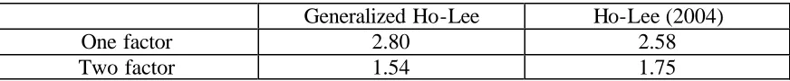
Figure 1. % Average Error (e) of the Estimation of the Swaption Prices
Generalized Ho-Lee Ho-Lee (2004)
One factor 2.80 2.58
Two factor 1.54 1.75
Next we investigate the error of each of the swaption in the estimation. The results are reported in Appendix C. For the one factor model, the generalized model can better explain the swaptions with long time to expiration and relatively short tenor. This result shows that negative interest rates of the normal interest rate model in the distribution of the relative short term rates at a long horizon date significantly and adversely affect the swaption pricing.
For the two factor models, the generalized Ho-Lee model has less estimation errors for the near term options. We will see later that the generalized model provides a better measure of implied term structure of volatilities.
4. Comparison of the Term Structure of Volatilities
The calibration procedure determines the implied term structure of volatilities for both models by estimating the parameters σ σ α α0, ∞, 0, ∞ , where the term structure of volatilities is given by
0 0
( )n ( n)exp( n)
σ = σ σ α− ∞+ −α∞ +σ∞ (62)
Figure 2. Estimated Parameters of the Term Structures of Volatilities for the 1 Factor Models
0
σ α0 α∞ σ∞
Generalized HL 0.482795 0.0000241 0.3007534 0.1835946
Normal HL 0.515295 -0.0004262 0.3337532 0.1425341
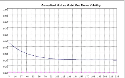
Figure 3. Generalized One Factor Ho Lee
One Factor Ho-Lee
Ho-Lee Model Volatilities (010204)
0.00 0.10 0.20 0.30 0.40 0.50 0.60 0.70 0.80 0.90 1.00
1 14 27 40 53 66 79 92 105 118 131 144 157 170 183 196 209 222 235
vol 1
vol2
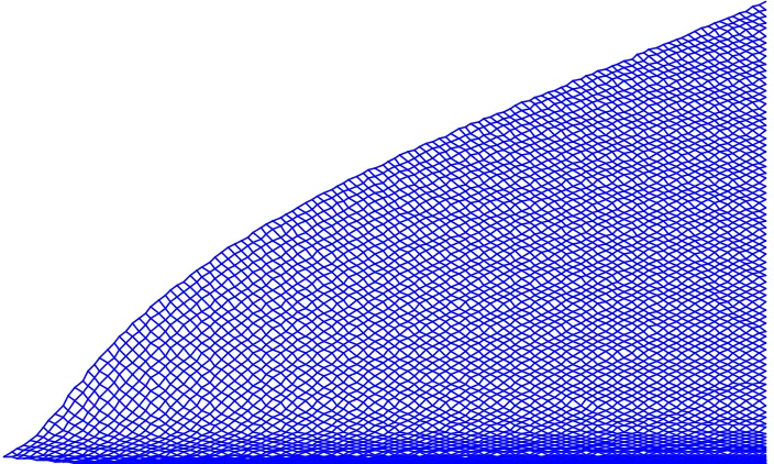
[image:20.612.83.530.478.580.2]Figure 3 depicts the term structure of volatilities of the generalized Ho- Lee model. The x-axis is the number of months and the y-x-axis measures the yields. The figure shows that the volatility curve decay occurs mostly in the first ten years. We now compare the term structures of volatilities of the two factor models.
Figure 4. The Estimated Parameters of the 2 Factor Models
1st Factor σ0 α0 α∞ σ∞
Generalized HL 0.5133690 0.0351239 0.0907066 0.0210815
Normal HL 0.5155230 0.0000400 0.3352112 0.1425682
2nd Factor σ0 α0 α∞ σ∞
Generalized HL 0.188918 0.0032930 0.0398720 0.0918580
Normal HL 0.074401 0.0001833 0.0002020 0.0572000
The model results are consistent with Litterman and Scheinkman results showing that one yield curve movement is the parallel movement, which is the second factor according to the generalized Ho-Lee model. The second yield curve movement is the slope movement, which is depicted by the first factor of our model. Our first factor shows that the short term portion of the yield curve tends to move more than the long term portion of the yield curve. This result also shows the striking difference between the generalized Ho-Lee model and the Ho-Lee normal model. The main difference is that the generalized Ho-Lee model allows for higher estimated volatilities. This is because Ho-Lee normal uses a lower volatility to accommodate the negative interest rates in order to fit the swaption
Generalized Ho-Lee Model One Factor Volatility
0.00 0.10 0.20 0.30 0.40 0.50 0.60 0.70 0.80 0.90 1.00
prices, when the market does not assume the significant presence of negative interest rates in the swaption pricing. Therefore, the generalized Ho-Lee model provides a more realistic estimation of the implied market volatilities.
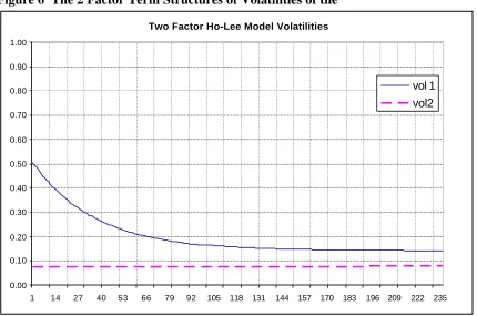
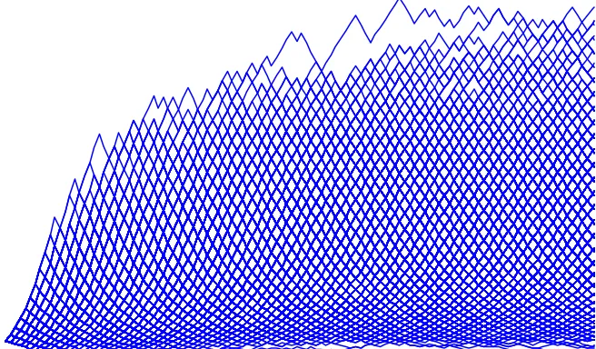
Figure 5 The 2 Factor Term Structures of Volatilities
Two Factor Generalized Ho-Lee Model Volatilities
0.00 0.10 0.20 0.30 0.40 0.50 0.60 0.70 0.80 0.90 1.00
1 14 27 40 53 66 79 92 105 118 131 144 157 170 183 196 209 222 235
Figure 6 The 2 Factor Term Structures of Volatilities of the
Two Factor Ho-Lee Model Volatilities
0.00 0.10 0.20 0.30 0.40 0.50 0.60 0.70 0.80 0.90 1.00
1 14 27 40 53 66 79 92 105 118 131 144 157 170 183 196 209 222 235
vol 1 vol2
Note the steeply downward sloping term structure of volatilities in both models, showing that the prices of the swaptions require the mean reversion interest rate movements.
E. Model Results
1. The Yields of the Zero Coupon Bonds
Given the above model, we can now determine the closed form solutions of the multi-factor interest rates. For clarity of the exposition, we will present the results for the one factor model. The extension of the one-factor model to the m- factor model is straightforward.
By definition, the yield of a T-period bond at node (n,i) is given by 1
( ) log ( )
n n
i i
R T P T
T t
= −
∆ . (63)
Using equation (63) and equation (34), we can derive the yield of the T year bond at each nodel (n,i). It is given below:
1 1
1 0
1
1 0 0
(1 ( ))
( )
( ) log log log ( )
( ) (1 ( ))
k
n i
n n
i k j
k j
n k P n T
R T T t T
P n n k T
δ δ
δ
− −
− −
= =
+ −
+
∆ = − − −
+ − +
∑
∑
(64)
1
1 0
1 0 0
(1 ( ))
( 1)
log log log
( ) (1 ( 1))
k
n i
n n
i k j
k j
n k P n
R t
P n n k
δ δ
δ
−
−
= =
+ −
+
∆ = − − −
+ − +
∑
∑
(65)For illustration, the one period yield for n=1 are:
1
0 0
0
(2) 2
log log
(1) (1 )
P R t
P δ
∆ = − −
+ (66)
1 0
1 0 0
0
(2) 2
log log log
(1) (1 )
P R t
P δ δ
∆ = − − −
+ (67)
The model is used to calculate the interest rates at each node point of the lattices. They are depicted below.
[image:23.612.206.519.82.230.2]2. Distribution of Interest Rates
Figure 7. One Month Rate on the Lattice of the Ho Lee Normal Model
Figure 8. One Month Interest Rate on the Lattice of the Generalized Ho Lee Model
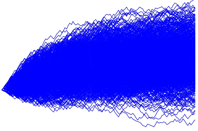
Figure 9. Randomly Simulated Paths of the 2 –Factor Generalized Ho-Lee Model
Figure 10. Randomly Simulated Paths from the 2 Factor Ho-Lee Model (2004)
F. Implications of the Model and the Conclusions
This paper presents an interest rate model that has four desirable attributes: (1) A recombining lattice model for accurate price of American and some Asian options, (2) A multifactor model to capture the yield curve shape movements, (3) A state-time dependent term structure of volatilities that ensures mean-reversion, non- negative interest rates and not unacceptably high interest rate levels, (4) A arbitrage-free model that takes the yield curve as given.
The model combining these attributes has a broad range of applications. The model can enhance the traditional applications of valuation models in trading, portfolio management, hedging, measuring key rate durations, convexities and other parametrics for measuring risks. The model can also meet the urgent needs of the financial markets in recent years.
challenges in the specifications the interest rate model that is a key component of many valuation and risk models.
For these reasons, financial engineers, auditors and regulators prefer the interest rate models to have the following properties: (1) The interest rate scenarios should be consistent with historical experiences, like, exhibiting non-negative interest rates, possible inverted yield curve, and mean reversion of interest rate level. (2) An ability to value a broad range of securities and balance sheet items accurately and the model can be calibrated to a broad range of marketable securities, not just swaptions or caps/floors, and can provide all the discount function and the term structure of volatilities at each node. (3) The model is transparent and results can be duplicated quite readily. Our multifactor interest rate model, with the forward volatilities being both state and time dependent can address all these requirements. We now discuss each requirement in turn.
When the interest rate model can generate the scenarios consistent to the historical experience, risk managers can relate the fair valuation of financial instruments with the stress scenarios. In managing the downside risk of a position, like using the Value at Risk measures, risk managers often need to better understand the distributions of the interest rates in the extreme cases as simulated by the valuation model. The proposed model can provide the realistic scenarios even in the extreme cases. The proposed model enables the risk managers to study the pathwise values of a portfolio of interest rate contingent claims based on a certain confidence level, where this model can provide reasonable extreme scenarios. (The pathwise value is defined as the present value of the cashflows along an interest rate path.)
interest rate. As long as the users of the model agree on these parameters, they should derive the same model results, and the model can be used for a broad range of contingent claims as discussed above. Any model that requires Monte-Carlo simulations like the BGM (Jackel and Rebonato (2000)) or the string models, or the construction of the lattice requiring numerical procedures in pruning the tree like Hull-White, or numerical methods in building an interest rate tree like Black Derman and Toy would not be able to offer a transparent specification of the model.
Finally, in research literature, the Ho-Lee model (1986) is often cited as simply an arbitrage- free model, a model that can be equivalently expressed in a continuous time framework. This model shows that the Ho-Lee model (1986) can be extended to the proposed model, which has more analytical structure than a continuous time arbitrage-free model. Specifically, the model specifies the discount function and term structure of volatilities at each node point, such that, at any node point, these discount functions in turn satisfy all arbitrage- free conditions. Such analytical structure not only offers a broader range of applications, it can be exploited for other applications.
References
Black F., E. Derman, and W. Toy (1990) “A one factor model of interest rates and its application to treasury bond options,” Financial Analysts Journal, Vol.46, 33-39.
Black F., and P. Karasinski (1991) “Bond and option pricing when short rates are lognormal” Financial Analysts Journal, Vol.47, 52-59.
Brace A., Gatarek D., Musiela M (1997) “The market model of interest rate dynamics” Mathematical Finance, Vol.7, 127-155
Cheyette, Oren (1997) “Interest rate models” In Advances in Fixed Income Valuation, Modeling and Risk Management, edited Frank J. Fabozzi. Frank J. Fabozzi Associates. New Hope, Pennsylvania.
Cox, Ingersoll and Ross (1985) “A theory of term structure of interest rates” Econometrica, Vol.53, 363-384.
Grant, Dwight and Gautan Vora (1999) “Implementing no-arbitrage term structure of interest rate models in discrete time when interest rates are normally distributed” Journal of Fixed Income, Vol. 8, no. 4, 85-98.
Harrison J. M. and d. M. Kreps (1979) “Martingales and arbitrage in multi-period securities markets,” Journal of Economic Theory, Vol.20, 381-408.
Ho, Thomas (1992), “Managing Illiquid Bonds and the Linear Path Space” Journal of Fixed Income, Vol.2, no.1, 80-94.
Ho, Tho mas and Sang Bin Lee (1986) “Term structure movements and pricing interest rate contingent claims” The Journal of Finance, Vol.41, no 5, 1011-1029.
Ho, Thomas and Sang Bin Lee (2004a) The Oxford Guide to Financial Modeling, The Oxford University Press, New York
Ho, Thomas and Sang Bin Lee (2004b) “A Closed-Form Multifactor Binomial Interest Rate Model” Journal of Fixed Income, Vol.14, no,1, 8-16.
Hull J. and White A. (1990) “Pricing interest rate derivative securities”, The Review of Financial Studies, Vol.3, no.4, 573-592.
Jäckel, Peter and Riccardo Rebonato (2000), “Linking Caplet and Swaption Volatilities in a BGM/J Framework: Approximate Solutions”, Quantitative Research Centre, The Royal Bank of Scotland,
Litterman, R., and J. A. Scheinkman (1991) “Common factors affecting bond returns” Journal of Fixed Income, Vol.1, no.1, 54-61
Longstaff, F., P. Santa-Clara, and E. Schwartz (2000) “The relative valuation of caps and swaptions: theory and empirical evidence” working paper. The Anderson School of UCLA September.
Appendix A
Proof of Proposition 1
The discount function with the time to maturity T at time n and state i
1 1
1 0
1
1 0 0
(1 ( ))
( )
( ) ( )
( ) (1 ( ))
k
n i
n n
i k j
k j
n k P n T
P T T
P n n k T
δ δ δ − − − − = = + − + = + − +
∏
∏
(A.1)The discount function with the time to maturity 1 at time n and state i
1 1
1 0
1
1 0 0
(1 ( ))
( 1)
(1) (1)
( ) (1 ( 1))
k
n i
n n
i k j
k j
n k P n
P
P n n k
δ δ δ − − − − = = + − + = + − +
∏
∏
(A.2)Divide Equation (A.1) by Equation (A.2) to get ( 1)
(1) n i n i P n P + ( 1) (1) n i n i P n P + = 1 1 1 0 0 1 1 1 1 0 0 ( )
(1 ( 1))
( )
( 1) (1 ( ))
(1) i n j k n j i k n k j j T n k
P n T
P n n k T
δ δ δ δ − − − = − − − = = + − + + + + − +
∏
∏
∏
(A.3)The discount function with the time to maturity T-1 at time n+1and state i
1
1 1
1 0
1
1 0 0
(1 ( 1 ))
( 1 1)
( 1) ( 1)
( 1) (1 ( 1 1))
k
n i
n n
i k j
k j
n k
P n T
P T T
P n n k T
δ δ δ − + − + − = = + + − + + − − = −
+
∏
+ + − + −∏
(A.4)=
1 1
0 0
1
1 0 0 0
(1 ( 1 )) (1 ( 1 1))
( 1 1)
( 1)
( 1) (1 ( 1 1)) (1 ( 1 1 1))
k n n i n j k n k j
n k n n
P n T
T
P n n k T n n T
δ δ δ δ δ − − − = = + + − + + − − + + − • − +
∏
+ + − + − + + − − + −∏
= 1 1 0 0 11 0 0 0
(1 ( 1 )) (1 (0))
( )
( 1)
( 1) (1 ( )) (1 ( 1))
k n n i n j k n k j n k
P n T
T
P n n k T T
δ δ δ δ δ − − − = = + + − + + • − +
∏
+ − + + −∏
= 1 1 1 0 1 11 0 0 0 1
( ) (1 ( 1))
(1 ( 1 ))
( ) 2
( 1) (1 ( )) (1 ( 1)) (1 ( ))
n n
k
n i
j j
k n n n
k j j j
T T
n k
P n T
P n n k T T T
δ δ
δ
δ δ δ δ
− − − − − = = + + − + + − + • +
∏
+ − + + −∏
+ 11 1 (1 ( 1))
( ) ( 1)
(1 ( 1))
n j
n n n
j j j n
j
T
T T
T δ
δ δ δ
δ
+
− = − − + −
+ −
Q from Equation (6)
=
1
1 1
0
1 1
1 0 0
( )
(1 ( 1 ))
( ) 2
( 1) (1 ( )) (1 ( 1))
n k
n i
j
k n n
k j j i
T
n k
P n T
P n n k T T
δ δ
δ δ δ
− − − − − = = + + − + •
+
∏
+ − +∏
+ − (A.5)1 ( ) 2
( 1)
(1) (1 ( 1))
n
n i
i n n
i i
P T P T
P δ T
+ − =
+ − (A.6)
Similarly, we can show that
1 1
( ) 2 ( 1)
( 1)
(1) (1 ( 1))
n n
n i i
i n n
i i
P T T
P T P T δ δ + + − − =
+ − (A.7)
Plugging Equation (A.6) and Equation (A.7) into Equation (44), we can see that Equation (44) holds.
1 1
1
1
( ) ( ( 1) ( 1))
2
n n n n
i i i i
P T = P P + T− +P++ T − (44)
as required.
For the two factor model, we can show that
, ,1 ,2
1 1, 1
, ,1 ,2
( ) 2 ( 1) 2 ( 1)
( 1)
(1) (1 ( 1)) (1 ( 1))
n n n
i j i j
n
i j n n n
i j i j
P T T T
P T
P T T
δ δ δ δ + + + − − − =
+ − + − (A.8)
, ,1
1 1,
, ,1 ,2
( ) 2 ( 1) 2
( 1)
(1) (1 ( 1)) (1 ( 1))
n n
i j i
n
i j n n n
i j i j
P T T
P T
P T T
δ δ δ + + − − =
+ − + − (A.9)
, ,2
1 , 1
, ,1 ,2
( ) 2 2 ( 1)
( 1)
(1) (1 ( 1)) (1 ( 1))
n n
i j j
n
i j n n n
i j i j
P T T
P T
P T T
δ δ δ + + − − =
+ − + − (A.10)
, 1
,
, ,1 ,2
( ) 2 2
( 1)
(1) (1 ( 1)) (1 ( 1))
n i j n
i j n n n
i j i j
P T P T
P δ T δ T
+
− =
+ − + − (A.11)
From Equation (A.8), (A.9), (A.10) and (A.11), we can see that Equation (A.12) holds.
1 1 1 1
, , 1, 1 1, , 1 ,
1
( ) ( ( 1) ( 1) ( 1) ( 1))
4
n n n n n n
i j i j i j i j i j i j
P T = P P++ + T− + P++ T− + P ++ T− + P + T−
(A.12)
Appendix B Swaption Black Volatilities
Swap Tenor (years)
Option Term
(years) 1yr 2yr 3yr 4yr 5yr 6yr 7yr 8yr 9yr 10yr