BIS Papers No 25 Zero-coupon yield curves: technical documentation

(1)

BIS Papers

No 25

Zero-coupon yield curves:

technical documentation

Monetary and Economic Department

(2)

This volume was originally prepared following a meeting on estimation of zero-coupon yield curves held at the Bank for International Settlements in June 1996, and the papers are technical in character. This volume is a revised version with updated papers from the reporting central banks.

Requests for copies of publications, or for additions/changes to the mailing list, should be sent to: Bank for International Settlements

Press & Communications CH-4002 Basel, Switzerland E-mail: publications@bis.org

Fax: +41 61 280 9100 and +41 61 280 8100

(3)

Zero-coupon yield curves estimated by central banks

Introduction

Following a meeting on the estimation of zero-coupon yield curves held at the BIS in June 1996, participating central banks have since been reporting their estimates to the Bank for International Settlements. The BIS Data Bank Services provide access to these data, which consist of either spot rates for selected terms to maturity or represent estimated parameters from which spot and forward rates can be derived. In the case estimated parameters are reported, the Data Bank Services provides, in addition to the parameters also the generated spot rates.

The purpose of this document is to facilitate the use of these data. It provides information on the reporting central banks’ approaches to the estimation of the zero-coupon yield curves and the data transmitted to the BIS Data Bank. In most cases, the contributing central banks adopted the so-called Nelson and Siegel approach or the Svensson extension thereof. A brief overview of the relevant estimation techniques and the associated mathematics is provided below. General issues concerning the estimation of yield curves are discussed in Section 1. Sections 2 and 3 document the term structure of interest rate data available from the BIS. The final section provides examples of estimated parameter and selected spot and forward rates derived thereof. A list of contacts at central banks can be found after the references. The remainder of this document consists of brief notes provided by the reporting central banks on approaches they have taken to estimate the yield curves.

Since the last release of this manual in March 1999 there have been four major changes: Switzerland started to report their estimates of the yield curve to the BIS in August 2002. Furthermore, Sweden began to use a new estimation method in 2001, the United Kingdom since September 2002 and Canada since January 2005. These changes are included in Tables 1 and 2.

1. Zero-coupon

yield

curve estimation techniques

The estimation of a zero-coupon yield curve is based on an assumed functional relationship between either par yields, spot rates, forward rates or discount factors on the one hand and maturities on the other. Discount factors are the quantities used at a given point in time to obtain the present value of future cash flows. A discount function dt,m is the collection of discount factors at time t for all maturities

m. Spot rates st,m, the yields earned on bonds which pay no coupon, are related to discount factors

according to:

(

s m

)

dt,m =exp− t,m and tm dtm m

s, log ,

1 −

= (1)

Because spot interest rates depend on the time horizon, it is natural to define the forward rates ft,m as

the instantaneous rates which, when compounded continuously up to the time to maturity, yield the spot rates (instantaneous forward rates are, thus, rates for which the difference between settlement time and maturity time approaches zero):

∫

−

= m

m

t f u du

m s

0

, ( )

1

(2) or, equivalently:

⎥⎦ ⎤ ⎢⎣

⎡−

=

_∫

m

t f u du

d

0

(6)

These relations can be inverted to express forward rates directly as a function of discount factors or spot rates: m t m t m

t s ms

f, = , + &, and

m t m t m t d d f , , , & −

= (4)

where dots stand for derivatives with respect to time to maturity.

However, the general absence of available pure discount bonds that can be used to compute zero-coupon interest rates presents a problem to practitioners. In other words, zero zero-coupon rates are rarely directly observable in financial markets. Attempting to extract zero-coupon rates from the prices of those risk-free coupon-bearing instruments which are observable, namely government bonds, various models and numerical techniques have been developed. Such models can broadly be categorised into parametric and spline-based approaches, where a different trade-off between the flexibility to represent shapes generally associated with the yield curve (goodness-of-fit) and the smoothness characterizes the different approaches. These main modelling approaches are now briefly discussed below.

Parametric Models

The underlying principle of parametric models, also referred to as function-based models, is the specification of a single-piece function that is defined over the entire maturity domain. Whilst the various approaches in this class of models advocate different choices of this function, they all share the general approach that the model parameters are determined through the minimisation of the squared deviations of theoretical prices from observed prices.

The Nelson and Siegel method

The method developed by Nelson and Siegel (1987) attempts to estimate these relationships by fitting for a point in time t a discount function to bond price data by assuming explicitly the following function form for the instantaneous forward rates:

⎟ ⎟ ⎠ ⎞ ⎜ ⎜ ⎝ ⎛ τ − τ β + ⎟ ⎟ ⎠ ⎞ ⎜ ⎜ ⎝ ⎛ τ − β + β = 1 , 1 , 2 , 1 , 1 , 0 ,

, exp exp

t t t t t t m t m m m

f (5)

In this equation m denotes time to maturity, t the time index and βt,0, βt,1, βt,2 and τt,1 are parameters to be estimated.1 The zero-coupon or spot interest rate curve sm can be derived by integrating the

forward rate curve:

⎟ ⎟ ⎠ ⎞ ⎜ ⎜ ⎝ ⎛ ⎟⎟ ⎠ ⎞ ⎜⎜ ⎝ ⎛ τ − − ⎟⎟ ⎠ ⎞ ⎜⎜ ⎝ ⎛ τ ⎟ ⎟ ⎠ ⎞ ⎜ ⎜ ⎝ ⎛ ⎟⎟ ⎠ ⎞ ⎜⎜ ⎝ ⎛ τ − − β + ⎟⎟ ⎠ ⎞ ⎜⎜ ⎝ ⎛ τ ⎟ ⎟ ⎠ ⎞ ⎜ ⎜ ⎝ ⎛ ⎟⎟ ⎠ ⎞ ⎜⎜ ⎝ ⎛ τ − − β + β = − − 1 1 1 1 2 1 1 1 1

0 1 exp 1 exp exp

m m

m

sm (6)

which is equivalent to:

(

)

_⎟⎟ ⎠ ⎞ ⎜⎜ ⎝ ⎛ τ − β − ⎟ ⎟ ⎠ ⎞ ⎜ ⎜ ⎝ ⎛ ⎟⎟ ⎠ ⎞ ⎜⎜ ⎝ ⎛ τ − − τ β + β + β = 1 2 1 1 2 1

0 1 exp exp

m m

m

sm (7)

For long maturities, spot and forward rates approach asymptotically the value β0 which must be positive. (β0 + β1) determines the starting value of the curve at maturity zero; β1 thus represents the deviation from the asymptote β0. In addition, (β0 + β1) must also be positive. The remaining two parameters β2 and τ1 are responsible for the “hump”. The hump’s magnitude is given by the absolute size of β2 while its direction is given by the sign: a negative sign indicates a U-shape and a positive sign a hump. τ1, which again must be positive, determines the position of the hump.

(7)

The Svensson method

To improve the flexibility of the curves and the fit, Svensson (1994) extended Nelson and Siegel’s function by adding a further term that allows for a second “hump”. The extra precision is achieved at the cost of adding two more parameters, β3 and τ2, which have to be estimated. The instantaneous forward rates curve thus becomes:

⎟⎟ ⎠ ⎞ ⎜⎜ ⎝ ⎛ τ − τ β + ⎟⎟ ⎠ ⎞ ⎜⎜ ⎝ ⎛ τ − τ β + ⎟⎟ ⎠ ⎞ ⎜⎜ ⎝ ⎛ τ − β + β = 2 2 3 1 1 2 1 1

0 exp exp exp

m m

m

fm (8)

with β3 and τ2 having the same characteristics as β2 and τ1 discussed above. Again, to derive the spot rates curve the instantaneous forward rates curve is integrated:

⎟ ⎟ ⎠ ⎞ ⎜ ⎜ ⎝ ⎛ ⎟⎟ ⎠ ⎞ ⎜⎜ ⎝ ⎛ τ − − ⎟⎟ ⎠ ⎞ ⎜⎜ ⎝ ⎛ τ ⎟ ⎟ ⎠ ⎞ ⎜ ⎜ ⎝ ⎛ ⎟⎟ ⎠ ⎞ ⎜⎜ ⎝ ⎛ τ − − β + ⎟ ⎟ ⎠ ⎞ ⎜ ⎜ ⎝ ⎛ τ − ⎟ ⎟ ⎠ ⎞ ⎜ ⎜ ⎝ ⎛ ⎟ ⎟ ⎠ ⎞ ⎜ ⎜ ⎝ ⎛ τ − − β + β = − − 1 1 1 1 2 1 1

0 1 exp 1 exp exp

1 1 m m m m m s_m ⎟ ⎟ ⎠ ⎞ ⎜ ⎜ ⎝ ⎛ ⎟⎟ ⎠ ⎞ ⎜⎜ ⎝ ⎛ τ − − ⎟⎟ ⎠ ⎞ ⎜⎜ ⎝ ⎛ τ ⎟ ⎟ ⎠ ⎞ ⎜ ⎜ ⎝ ⎛ ⎟⎟ ⎠ ⎞ ⎜⎜ ⎝ ⎛ τ − − β + − 2 1 2 2

3 1 exp exp

m m

m

(9)

For zero-coupon bonds, spot rates can be derived directly from observed prices. For coupon-bearing bonds usually their “yield to maturity” or “par yield” only is quoted. The yield to maturity is its internal rate of return, that is the constant interest rate rk that sets its present value equal to its price:

∑

= +

= n

i _k t

i k i r CF P

1(1 )

(10) where Pk is the price of bond k which generates n cash-flows CF at periods tj (i = 1, 2, .. , n). These

cash flows consist of the coupon payments and the final repayment of the principal or face value. Yields to maturity on coupon bonds of the same maturity with different coupon payments are not identical. In particular, the yield to maturity on a coupon-bearing bond differs from the yield to maturity - or spot rate - of a zero-coupon bond of the same maturity. Nevertheless, if the cash flow structure of a bond trading at the market (“at par”) is known, it is possible to derive from estimated spot rates uniquely the coupon bond’s theoretical yield to maturity, ie the rate the bond would require in order to trade at its face value (“at par”). Drawing on the spot rates st,m, the price equation can be expressed

as: m m t m m t t t k s V s C s C s C P ) 1 ( ) 1 ( ... ) 1 ( ) 1

( 2 _, _,

2 , 1 , + + + + + + + +

= (11)

where C represents the coupon payments and V the repayment of the principal. The yield to maturity of a coupon-bearing bond is therefore an average of the spot rates which, in general, varies with the term to maturity.

To derive the term structure of interest rates, the discount function is estimated by applying a (constrained) non-linear optimisation procedure to data observed on a trade day. More important than the choice of a particular optimisation method (eg maximum likelihood, non-linear least squares, generalised method of moments) is the decision whether the (sum of squared) yield or price errors should be minimised. If one is primarily interested in interest rates, it suggests itself to minimise the deviation between estimated and observed yields. In this case the estimation proceeds in two stages: first, the discount function dt,m is used to compute estimated prices and, secondly, estimated yields to

maturity are calculated by solving the following equation for each coupon-bearing bond k:

(

r i

)

V

(

r m

)

C

P k k

m i

k =

∑

− + −

=

exp exp

1

(12) At both stages, the starting point is from pre-selected values for the relevant parameters and to run

(8)

price errors than yield errors, as this only requires finding a solution for the first stage. Unfortunately, minimising price errors can lead to large yield errors for financial instruments with relatively short remaining term to maturity. Considering how yield, price and term to maturity of a bond are related, it is not surprising to observe this heteroscedasticity problem: drawing on the concept of duration,2 the elasticity of the price with respect to one plus the yield is equal to the duration of the bond. A given change in the yield corresponds to a small/large change in the price of a bond with a short/long term to maturity or duration. Fitting prices to each bond, given an equal weight irrespective of its duration, leads to over-fitting of the long-term bond prices at the expense of the short-term prices. One approach to correct for this problem is to weight the price error of each bond by a value derived from the inverse of its duration.

Other factors can also contribute to fairly large yield errors at the short end of the term structure. For instance, the trading volume of a bond can decrease considerably when it approaches its maturity date. The quoted price for such a bond may not accurately reflect the price at which trading would take place. For such reasons it may be appropriate to exclude price data of bonds close to expiration when fitting term structures.

Spline-based Models

Rather than specifying a single functional form over the entire maturity range, spline-based methods fit the yield curve by relying on a piecewise polynomial, the spline function3, where the individual segments are joined smoothly at the so-called knot points. Over a closed interval, a given continuous function can be approximated by selecting an arbitrary polynomial, where the goodness-of-fit increases with the order of the polynomial. Higher-order polynomials, however, quite frequently display insufficient smoothing properties. This problem can be avoided by relying on a piecewise polynomial whereby the higher-order polynomial is approximated by a sequence of lower-order polynomials. Consequently, spline functions are generally based on lower-order polynomials (mostly quadratic or cubic). A cubic spline, for instance, is a piecewise cubic polynomial restricted at the knot points such that their levels and first two derivatives are identical. One parameter corresponds to each knot in the spline.

The “smoothing splines” method

This method developed by Fisher, Nychka and Zervos (1995) represents an extension of the more traditional cubic spline techniques (eg Vasicek and Fong (1982)). In the case of “smoothing splines” the number of parameters to be estimated is not fixed in advance. Instead, one starts from a model which is initially over-parameterised. Allowing for a large number of knot points guarantees sufficient flexibility for curvature throughout the spline. The optimal number of knot points is then determined by minimizing the ratio of a goodness-of-fit measure to the number of parameters. This approach penalizes for the presence of parameters which do not contribute significantly to the fit. It is not convenient to draw on the (varying number of) parameters in disseminating yield curve information. There is a broad range of spline-based models which use this “smoothing method” pioneered by Fisher et al. The main difference among the various approaches simply lies in the extent to and fashion by which the smoothing criteria are applied to obtain a better fix. The “variable penalty roughness” (VRP) approach recently implemented by the Bank of England allows the “roughness” parameter to vary with the maturity, permitting more curvature at the short end.4

2 _{Recall that the duration of a coupon bond is equal to its maturity. Assuming a flat yield curve, the sensitivity of a} zero-coupon bond to a change in the term structure should be directly proportional to its maturity. A change in the interest rate divided by one minus the interest rate of 1% corresponds to a change in the price of 1% of a bond with a maturity of one year and of 10% of a 10-year bond.

3_{Spline functions, such as basis or B-splines, are used in the context of yield curve estimation. At times there exists some} confusion among practitioners between spline functions and spline-based interpolation. While the former technique uses polynomials in order to approximate (unknown) functions, the latter is simply a specific method to interpolate between two data points.

4

(9)

Generally, the estimation method largely depends on intended use of data: no-arbitrage pricing and valuation of fixed-income and derivative instruments vs information extraction for investment analytical and monetary policy purposes. One of the main advantages of spline-base techniques over parametric forms, such as the Svensson method, is that, rather than specifying a single functional form to describe spot rates, they fit a curve to the data that is composed of many segments, with the constraint that the overall curve is continuous and smooth.5

2. Provision of information on the term structure of interest rates

The term structure of interest rates, defined as the functional relationship between term to maturity and the spot interest rate of zero-coupon bonds, consists of an infinite number of points. In many respects forward interest rates are more interesting than spot rates, as implied by the spot rate curve or vice versa, as the former can pertain information about expected future time paths of spot rates. At any point along the maturity spectrum there exists an infinite number of forward rates which differ in terms of their investment horizon. The instantaneous forward rate represents just a special case, the one for which the investment horizon approaches zero.

Published information on term structure of interest rates usually consists of selected spot rates at discrete points along the maturity spectrum. Occasionally, these spot rates are complemented by a selection of specific forward interest rates.

Such limitations would be mitigated if information on the term structure of interest rates could be presented in terms of algebraic expressions from which spot and forward rates can be derived. This is straightforward for parsimonious approaches such as Nelson and Siegel and Svensson discerned above, for which spot and instantaneous forward rates can be calculated using the estimated parameters (β’s and τ’s).

Further information can be useful in interpreting the curves such as statistics on the quality of the fit, details on the debt instruments used in the estimations, and if and what kind of efforts were made to prevent that specific premia, eg tax premia, distort estimation results. Some of this information can be found below and in the notes provided by the central banks.

Comparability of central banks’ term structures of interest rates

To estimate the term structure of interest rates, most central banks reporting data have adopted either the Nelson and Siegel or the extended version suggested by Svensson. Exceptions are Canada, Japan, (in part) Sweden6, the United Kingdom, and the United States which all apply variants of the “smoothing splines” method.

Government bonds data are used in the estimations since they carry no default risk. Occasionally, central banks complement this information by drawing on money market interest rates or swap rates. Clearly, financial markets differ considerably in terms of the number of securities actively traded and their turnover, the variety of financial instruments and specific institutional features. Such differences can give rise to a variety of premia which should be taken into consideration in the estimation process but in practice this is difficult to do.

Premia induced by tax regulations are notoriously difficult to deal with. One could attempt to remove tax-premia from the observed prices/yields before they are used in estimations. In other instances it may be preferable to simply exclude instruments with distorted prices/yields from the data set. In cases where it is expected that tax distortions have only a minor impact on the estimation results the best approach may be to ignore this problem altogether. Occasionally, central banks prefer modifying the estimation approach instead of adjusting the data to deal with specific problems (see Table 1).

5

For example, at the long end of the yield curve, the Svensson model is constrained to converge to a constant level, directly implying that the unbiased expectation hypothesis holds.

6

(10)

(11)

[image:11.595.84.542.115.686.2]

Table 1

The term structure of interest rates - estimation details

Central bank Estimation method

Minimised error

Shortest maturity in estimation

Adjustments for tax distortions

Relevant maturity spectrum

Belgium Svensson or

Nelson-Siegel

Weighted prices Treasury certificates: > few days

Bonds: > one year

No Couple of days

to 16 years

Canada Merrill Lynch

Exponential Spline

Weighted prices Bills: 1 to 12 months

Bonds: > 12 months

Effectively by excluding bonds

3 months to 30 years

Finland Nelson-Siegel Weighted prices ≥ 1 day No 1 to 12 years

France Svensson or

Nelson-Siegel

Weighted prices Treasury bills: all Treasury

Notes: : ≥ 1 month

Bonds: : ≥ 1 year

No Up to 10 years

Germany Svensson Yields > 3 months No 1 to 10 years

Italy Nelson-Siegel Weighted prices Money market

rates: O/N and Libor rates from 1 to 12 months

Bonds: > 1 year

No Up to 30 years

Up to 10 years (before February 2002)

Japan Smoothing splines

Prices ≥ 1 day Effectively by

price

adjustments for bills

1 to 10 years

Norway Svensson Yields Money market

rates: > 30 days

Bonds: > 2 years

No Up to 10 years

Spain Svensson

Nelson-Siegel (before 1995)

Weighted prices

Prices

≥ 1 day ≥ 1 day

Yes

No

Up to 10 years

Sweden Smoothing splines and

Svensson

Yields ≥ 1 day No Up to 10 years

Switzerland Svensson Yields Money market

rates: ≥ 1 day

Bonds: ≥ 1 year

(12)

[image:12.595.56.510.104.325.2]

Table 1 cont

The term structure of interest rates - estimation details

Central bank Estimation method

Minimised error

Shortest maturity in estimation

Adjustments for tax distortions

Relevant maturity spectrum

United Kingdom1

VRP (government nominal)

VRP (government real/implied inflation)

VRP (bank liability curve)

Yields

1 week (GC repo yield)

1.4 years

1 week

No

Up to around 30 years

United States Smoothing splines (two curves)

Bills:

weighted prices

Bonds: prices

–

≥ 30 days

No

Up to 1 year

1 to 10 years

1

The United Kingdom used the Svensson method between January 1982 and April 1998.

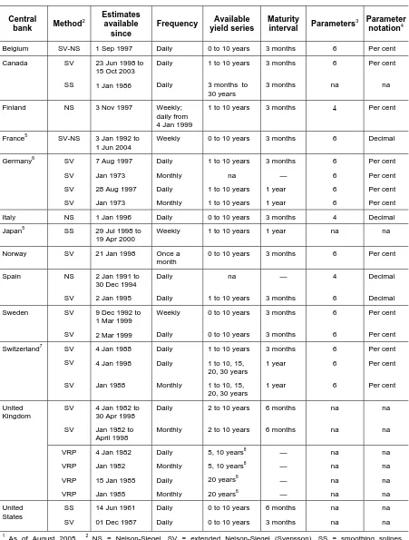
3. Zero-coupon yield curves available from the BIS

[image:12.595.54.513.110.325.2]

(13)

[image:13.595.88.539.100.695.2]

Table 2

The structure of interest rates available from the BIS Data Bank1

Central

bank Method

2 Estimates available

since

Frequency Available yield series

Maturity

interval Parameters

3 Parameter notation4

Belgium SV-NS 1 Sep 1997 Daily 0 to 10 years 3 months 6 Per cent

Canada SV

SS

23 Jun 1998 to 15 Oct 2003

1 Jan 1986

Daily

1 to 10 years

3 months to 30 years 3 months 3 months 6 na Per cent na

Finland NS 3 Nov 1997 Weekly; daily from 4 Jan 1999

1 to 10 years 3 months 4 Per cent

France5 SV-NS 3 Jan 1992 to 1 Jun 2004

Weekly 0 to 10 years 3 months 6 Decimal

Germany6 SV

SV

7 Aug 1997

Jan 1973

28 Aug 1997

Jan 1973

Daily

Monthly

Daily

Monthly

1 to 10 years

na

1 to 10 years

3 months — 1 year 1 year 6 6 6 6 Per cent Per cent Per cent Per cent

Italy NS 1 Jan 1996 Daily 0 to 10 years 3 months 4 Decimal

Japan5 _SS _{29 Jul 1998 to} 19 Apr 2000

Weekly 1 to 10 years 1 year na na

Norway SV 21 Jan 1998 Once a

month

0 to 10 years 3 months 6 Per cent

Spain NS

SV

2 Jan 1991 to 30 Dec 1994

2 Jan 1995

Daily

na

1 to 10 years

— 3 months 4 6 Decimal Decimal Sweden SV SV

9 Dec 1992 to 1 Mar 1999

2 Mar 1999

Weekly

Daily

0 to 10 years

3 months 3 months 6 6 Per cent Per cent

Switzerland7 SV

SV

4 Jan 1988

4 Jan 1998

Jan 1988

Daily

Monthly

1 to 10 years

1 to 10, 15, 20, 30 years

3 months 1 year 1 year 6 6 6 Per cent Per cent Per cent SV SV

4 Jan 1982 to 30 Apr 1998

Jan 1982 to April 1998

Daily

Monthly

2 to 10 years

6 months 6 months na na na na United Kingdom VRP VRP VRP VRP

4 Jan 1982

Jan 1982

15 Jan 1985

Jan 1985

Daily

Monthly

Daily

Monthly

5, 10 years8

20 years8

— — — — na na na na na na na na United States SS SV

14 Jun 1961

01 Dec 1987

Daily

0 to 10 years

6 months 3 months na na na na 1

As of August 2005. 2 NS = Nelson-Siegel, SV = extended Nelson-Siegel (Svensson), SS = smoothing splines, VRP = variable roughness penalty. 3 Where there is an indication of a parameter there is also a BIS generated yield available on the BIS Data Bank. Moreover, “na” means that the country is transmitting estimated yields and not parameters. 4

(14)

4. Spot interest rates and forward rates derived from estimation

parameters

[image:14.595.59.510.317.650.2]

Spot interest rates and instantaneous forward rates can be derived directly from the equations for the Nelson-Siegel and Svensson approaches presented above: replace the parameters of the equations - β0, β1, β2 and τ1 in the Nelson and Siegel and β0, β1, β2, τ1, β3 and τ2 in the Svensson case - by their estimated values and evaluate the equations at terms to maturity m for which the spot or forward rates have to be derived (eg m = 1 for one year to maturity). Table 3 provides examples of estimated parameters and a selection of corresponding points on the term structures. For the calculation of spot and instantaneous forward rates, it is partly relevant if the term structure was estimated either in decimal or percentage notation; the only difference is that the β-parameters are rescaled by a factor of 100. Clearly, such rescaling has no impact on the location of the humps as determined by the τ-parameters. By setting β3 = 0 and τ2 to an arbitrary non-zero value (eg τ2 = 1), the Svensson equations can be used to derive spot and forward rates of term structures estimated by the Nelson and Siegel approach. Thus it is sufficient to implement just the two Svensson equations to derive the spot and instantaneous forward rates for both approaches.

Table 3

Spot interest rates and instantaneous forward rates derived from estimation parameters Estimation

parameters

Svensson (in percentage notation)

Nelson and Siegel (in decimal notation)

Nelson and Siegel (in percentage notation)

β0 5.82 0.0769 7.69

β1 –2.55 –0.0413 –4.13

β2 –0.87 –0.0244 –2.44

τ1 3.90 0.0202 2.02

β3 0.45 – –

τ2 0.44 – –

Term to maturity

Spot rate (%)

Forward

rate (%) Spot rate

Forward rate

Spot rate (%)

Forward rate (%)

0 3.27 3.27 0.0356 0.00356 3.56 3.56

1 year 3.61 3.78 0.0400 0.0444 4.00 4.44

15 months 3.65 3.84 0.0411 0.0465 4.11 4.65

18 months 3.69 3.91 0.0421 0.0486 4.21 4.86

21 months 3.72 3.98 0.0432 0.0506 4.32 5.06

2 years 3.76 4.05 0.0443 0.0526 4.43 5.26

5 years 4.17 4.80 0.0546 0.0683 5.46 6.83

10 years 4.68 5.45 0.0639 0.0758 6.39 7.58

∞ 5.82 5.82 0.0769 0.0769 7.69 7.69

(15)

References

Anderson, N, F Breedon, M Deacon, A Derry and G Murthy (1996): “Estimating and interpreting the yield curve”, John Wesley and Sons.

Anderson, N, F Breedon, M Deacon, A Derry, G Murthy and J Sleath (1999): “New estimates of the UK real and nominal yield curves”, Bank of England Quarterly Bulletin, November, pp 384-392. Cooper, N and J Steeley (1996): “G7 yield curves”. Bank of England, Quarterly Bulletin, May, pp 199-208.

Deutsche Bundesbank (1995): “The market of German Federal Securities”, Frankfurt am Main, July. Fama, E F and R R Bliss: “The information in long-maturity forward rates”. American Economic Review, LXXVII, pp 680-92.

Fisher, M, D Nychka and D Zervos (1995): “Fitting the term structure of interest rates with smoothing splines”, Board of Governors of the Federal Reserve System, Finance and Economics Discussion Series, 95-1.

McCulloch, J H (1971): “Measuring the term structure of interest rates”, Journal of Business, 44, pp 19-31.

McCulloch, J H (1975): “The tax adjusted yield curve”, Journal of Finance, 90, pp 811-30.

Estrella, A and F S Mishkin (1997): “The predictive power of the term structure of interest rates in Europe and the United States: Implications for the European Central Bank”, European Economic Review, 41, pp 1375-401.

James, J and Nick Webber (2000): “Interest Rate Modelling”, John Wiley and Sons Ldt.

Nelson, C R and A F Siegel (1987): “Parsimonious modeling of yield curves”, Journal of Business, 60, pp 473-89.

Seppälä, J and P Viertiö (1996): “The term structure of interest rates: estimation and interpretation”, Bank of Finland, Discussion Paper, No 19.

Schich, S T (1996): “Alternative specifications of the German term structure and its information content regarding inflation”, Deutsche Bundesbank, Economic Research Group, Discussion Paper, No 8, October.

Schich, S T (1997): “Estimating the German term structure”, Deutsche Bundesbank, Economic Research Group, Discussion Paper, No 4.

Svensson, L E O (1994): “Estimating and interpreting forward interest rates: Sweden 1992-4”, CEPR Discussion Paper Series, No 1051, October (also: NBER Working Paper Series, No 4871).

Ricart, R and P Sicsic (1995): “Estimating the term structure of interest rates from French data”, Banque de France, Bulletin Digest, No 22, October.

(16)

Contacts at central banks

National Bank of Belgium Research Department Boulevard de Berlaimont 14 B-1000 Bruxelles

Tel: +32 2 221 5441 Fax: +32 2 221 3162

Raf Wouters rafael.wouters@nbb.be

Bank of Canada

Financial Markets Department Wellington Street 234

Ottawa K1A 0G9 Canada

Tel: +1 613 782 7312 Fax: +1 613 782 8655

Scott Gusba sgusba@bankofcanada.ca

Bank of France

Economic Studies and Research Division

39, rue Croix-des-Petits-Champs F-75049 Paris CEDEX 01 Tel: +33 1 4292 9284 Fax: +33 1 4292 6292

Sanvi Avouyi-Dovi sanvi.avouyi-dovi@banque-france.fr

Bank of Finland Economics Department PO Box 160

FIN-00101 Helsinki Tel: +358 9 183 2467 Fax: +358 9 622 1882

Lauri Kajanoja Lauri.Kajanoja@bof.fi

Deutsche Bundesbank Department of Economics Wilhelm-Epstein-Strasse 14 D-60431 Frankfurt am Main Tel: +49 069 9566 8542 Fax: +49 069 9566 3082

Jelena Stapf Jelena.Stapf@bundesbank.de

Bank of Italy

Research Department Via Nazionale 91 I-00184 Roma

Tel: +39 06 4792 4108 Tel: +39 06 4792 3943 Fax: +39 06 4792 3723

Roberto Violi Antonio Di Cesare

(17)

Bank of Japan

Research and Statistics Department

Tokyo CPO Box 203 Tokyo 100-8630 Japan

Tel: +81 3 3277 3040 Fax: +81 3 5203 7436

Katsurako Sonoda katsurako.sonoda@boj.or.jp

Bank of Norway Department for Market Operations and Analysis Bankplassen 2

N-0107 Oslo Tel: +47 2231 6351 Fax: +47 2233 3735

Knut Eeg

Gaute Myklebust

knut.eeg@moa.norges-bank.no

gaute.myklebust@moa.norges-bank.no

Bank of Spain

Research Department Alcalá 50

E-28014 Madrid Tel: +34 91 338 5413 Fax: +34 91 338 6023

Ms Miriam Cordal mcordal@bde.es

Sveriges Riksbank Financial Markets Analysis Department of Monetary Policy Brunkebergstorg 11

S-103 37 Stockholm Tel: +46 8 787 0503 Fax: +46 8 210 531

Hans Dillén Carl-Fredrik Petterson

Hans.Dillen@riksbank.se

Carl-Fredrik.Petterson@riksbank.se

Swiss National Bank Statistics Section Börsenstrasse 15 CH-8022 Zürich Tel: +41 1 631 3963 Fax: +41 1 631 8112

Robert Müller Robert.Mueller@snb.ch

Bank of England Monetary Instruments and Market Division Threadneedle Street GB-London EC2R 8AH Tel: +44 207 601 4444 Fax: +44 207 601 5953

Mike Joyce Matthew Hurd

(18)

Board of Governors of the Federal Reserve System Monetary & Financial Markets Analysis (MFMA) 20th and C Streets, NW Mail Stop 68

Washington, DC 202551 USA

Tel: +1 202 452-3433 Fax: +1 202 452-2301

Jonathan Wright jonathan.h.wright@frb.gov

Bank for International Settlements

Data Bank Services Centralbahnplatz 2 CH-4002 Basel Tel: +41 61 280 8313 Fax: +41 61 280 9100

Christian Dembiermont

(19)

Technical note on the estimation procedure

for the Belgian yield curve

Michel Dombrecht and Raf Wouters1

The purpose of this note is to document the methodology and data used for the construction of the zero coupon yield curve that is daily estimated by the National Bank of Belgium. The yield curve is based on the functional form proposed by Nelson and Siegel (1985) and extended by Svensson (1994).

Theoretical model

The following functional form is used to represent the zero coupon yield curve:

⎥ ⎥ ⎥ ⎥ ⎥ ⎦ ⎤ ⎢ ⎢ ⎢ ⎢ ⎢ ⎣ ⎡ ⎟⎟ ⎠ ⎞ ⎜⎜ ⎝ ⎛ τ − − τ ⎟⎟ ⎠ ⎞ ⎜⎜ ⎝ ⎛ τ − − ∗ β + ⎥ ⎥ ⎥ ⎥ ⎥ ⎦ ⎤ ⎢ ⎢ ⎢ ⎢ ⎢ ⎣ ⎡ ⎟⎟ ⎠ ⎞ ⎜⎜ ⎝ ⎛ τ − − τ ⎟⎟ ⎠ ⎞ ⎜⎜ ⎝ ⎛ τ − − ∗ β + ⎥ ⎥ ⎥ ⎥ ⎥ ⎦ ⎤ ⎢ ⎢ ⎢ ⎢ ⎢ ⎣ ⎡ τ ⎟⎟ ⎠ ⎞ ⎜⎜ ⎝ ⎛ τ − − ∗ β + β = 2 2 2 3 1 1 1 2 1 1 1 0 exp exp 1 exp exp 1 exp 1 ) ( m m m m m m m m m

r (1)

The zero coupon yield r depends on the maturity of the bond (m) and the parameters β0, β1, β2, β3, τ1 and τ2. This function is used to define the discount factor d(m):

d(m) = exp

(

)

⎟

⎠ ⎞ ⎜

⎝

⎛₋ βτ

m m r 100 , , (2) Each bond price can then be approximated by the discounted sum of the coupon payments and final capital:

Pe(m) =

∑

(

)

= ⎟ ⎠ ⎞ ⎜ ⎝

⎛₋ βτ

m i i m r 1 100 , ,

exp ∗ Coupon + exp

(

)

⎟

⎠ ⎞ ⎜

⎝

⎛₋ βτ

m m r 100 , , _∗ 100 (3) The parameters β0, β1, β2, β3, τ1 and τ2 are estimated by minimising the sum of squared bond price

errors weighted by (1/Φ):

(

)

[

]

{

}

2

1 2 1 2 1 0 2 1 2 1 0 / , , , , , , , ,

∑

= Φ τ τ β β β − τ τ β β β n j j e j j P P Min (4) where Φ equals the duration ∗ price /(1 + yield to maturity) of the bond.

Application and data

The daily estimation is based on the market price of Treasury certificates and linear bonds: all outstanding Treasury certificates (with a maturity between days and one year) and all linear bonds or OLO’s in Belgian francs with a maturity longer than one year (excluding line 239) are included in the sample. This means that some 45 prices are considered, of which 18 bond prices and 27 Treasury

1

(20)

certificates. This sample is adjusted over time according to the information from specialists in the bond market.

The market prices of the bonds are corrected for the accrued interest calculated as a proportion of the coupon payment. There is no correction for the deviation between the day of trade (t) and the day of settlement (t + 3 for bonds and t + 2 for the Treasury certificates).

The estimation programme starts by estimating the parameters β0, β1, β2 and τ1 with fixed β3 = 0 and

τ2 = 1. Then the programme checks whether the estimation result improves by adding β3 and τ2. If these coefficients are not significant, the simple Nelson-Siegel formula is retained; otherwise, the extended Svensson formula is used.

References

Nelson, C R and A F Siegel (1985): “Parsimonious modeling of yield curves for US Treasury bills”, NBER Working Paper Series, no 1594.

Svensson, L E O (1994): “Estimating and interpreting forward interest rates: Sweden 1992-4”, NBER Working Paper Series, no 4871.

(21)

A technical note on the Merrill Lynch Exponential Spline model

as applied to the Canadian term structure

David Bolder, Scott Gusba, and David Stréliski1

The purpose of this note is to describe the methodology used by the Bank of Canada to construct the Government of Canada yield curve. We generate zero coupon curves daily, for maturities from 0.25 to 30.00 years, by applying an estimation method based on the Merrill Lynch Exponential Spline (MLES) model to a selection of Government of Canada Treasury bill and bond prices.2

1. Data

The two fundamental types of Canadian dollar-denominated marketable securities issued by the government of Canada are Treasury bills and Canada bonds. Treasury bills, which do not pay periodic interest but rather are issued at a discount and mature at their par value, are currently issued at three-, six- and 12-month maturities. Government of Canada bonds pay a fixed semi-annual interest rate and have a fixed maturity date. Issuance involves maturities across the yield curve with original terms of maturity at issuance of two, five, 10 and 30 years.3 Each issue is reopened several times to improve liquidity and achieve “benchmark status”.4_{Canada bonds are currently issued on a quarterly}

“competitive yield” auction rotation with each maturity typically auctioned once per quarter.5 In the interests of promoting liquidity, Canada has set targets for the total amount of issuance to achieve “benchmark status”; currently, these targets are CAD 7 billion to 10 billion for each maturity.

2. Data

filtering

Our goal is to select only those bonds that are indicative of the current market yields. As a result, we use a system of filters to omit bonds which create distortions in the estimation of the yield curve. • To avoid potential price distortions when large deviations from par exist, bonds that trade at

a premium or a discount of more than 500 basis points from their coupon are excluded.6 • Bonds with less than CAD 500 million outstanding are excluded in order to include only

those bonds with the requisite degree of liquidity. This amount was chosen in a fairly arbitrary manner to ensure a reasonable number of bonds in the sample.

• Canada benchmark bonds are the most actively traded Canada bonds in the marketplace and it is thus essential that the information contained in these bonds be incorporated into the yield curve.7

1 _{Analysts, Bank of Canada, Ottawa.}

2 _{For a more detailed description of the approach, see Bolder and Gusba (2002), or Bolder, Johnson and Metzler (2004).}

3 _{Canada eliminated three-year bond issues in early 1997; the final three-year issue was 15 January.}

4 _{A “benchmark” bond is analogous to an “on-the-run” US Treasury security in that it is the most actively traded security for a}

given maturity.

5_{Government of Canada bond yields are quoted on an actual/actual day count basis net of accrued interest. The accrued}

interest, however, is by market convention calculated on an actual/365 day count basis.

6_{This value of 500 basis points is intended to reflect a threshold at which the tax effect of a discount or premium is not}

(22)

• Additional “discretionary” filtering of bonds is possible. It should be noted, however, that the inclusion or exclusion of a bond is based on judgment and would occur after investigating the underlying reason for a problematic (or unusual) bond quote.

3. The

model

The Bank of Canada uses the Merrill Lynch Exponential Spline (MLES) model, developed by Li et al.8 The MLES model is a parametric model which specifies a functional form for the discount function, d(t), as

t k k

ke

z t

d −α

=

∑

= 9

1

)

( (1)

where zk (k = 1,...,9) and α are the parameters to be estimated.

Once a functional form for the discount function has been specified, a zero coupon interest rate function is derived. The zero coupon curve, z(t), is given by

t t d t

z( )=−(ln( ( ))/ (2)

4. The

estimation

The basic process of determining the optimal parameters for the discount function which best fits the bond data is outlined as follows:

• The sample of Government of Canada bond and Treasury bills is selected and the timing and magnitude of their cashflows are determined.

• The estimation involves 9 linear parameters (the zk), and one non-linear parameter (α). The

optimization normally takes less than one minute to complete. Maximum likelihood estimation is used. As a result of the fact that the discount function is a linear function of 9 of the 10 parameters, the majority of the maximum likelihood computations can be carried out as matrix multiplications, which are computationally efficient.

• Price residuals are calculated using theoretical Government of Canada security prices and the actual price data and inversely weighted by (modified) duration. The calculation of estimated prices is straightforward as the discount function permits us to discount any cashflow occurring throughout the term to maturity spectrum. The weighting on the i-th bond (wi) is given as follows:

i

i D

w =1/

where Di is the (modified) duration of the i-th bond.9

7_{As previously discussed, the new issues may require two or more reopenings to attain “benchmark status”. As a result, the}

decision as to whether or not a bond is a benchmark is occasionally a matter of judgment.

8 _{Li et al (2001)}

(23)

References

Bliss, R R Jr (1996): “Testing term structure estimation methods”, Federal Reserve Bank of Atlanta, Working Paper, no 96-12a, November.

Bolder, D, G Johnson and A Metzler (2004): “An Empirical Analysis of the Canadian Term Structure of Zero-Coupon Interest Rates”, Bank of Canada Working Paper No 2004-48.

Bolder, D and S Gusba (2002): “Exponentials, Polynomials, and Fourier Series: More Yield Curve Modelling at the Bank of Canada”, Bank of Canada Working Paper No 2002-29.

(24)

Notes on the estimation for the Finnish term structure

Lauri Kajanoja and Antti Ripatti1

1. Nelson and Siegel method as applied at the Bank of Finland

The daily term structure of interest rates for Finland is estimated using the methods developed by Nelson and Siegel (1987).2 Given the parameter vector, β, and maturity, m, the instantaneous forward rate is defined as follows:

⎟⎟ ⎠ ⎞ ⎜⎜ ⎝ ⎛

τ − τ

β + ⎟⎟ ⎠ ⎞ ⎜⎜ ⎝ ⎛

τ − β

+ β = β

1 1

2 1 1

0 exp exp

) ,

(m m m m

f (1)

The corresponding spot rate (zero coupon interest rate) is:

⎟⎟ ⎠ ⎞ ⎜⎜ ⎝ ⎛

τ − β

− τ

τ − − β + β + β = β

1 2

1 1 2

1

0 exp

/ ) / ( exp 1 ) ( ) ,

( m

m m m

s (2)

The parameters β0 (labelled as BETA0 in the database), β1 (BETA1), β2 (BETA2), and τ1 (TAU1) are estimated using the following assumptions:

• The estimation is based on the minimisation of the yield errors (based on the maximum likelihood method assuming that yield errors follow normal distribution).

• The spot curve is usually but not always forced to pass the overnight rate. When it is, the instantaneous forward rate with zero maturity corresponds to the overnight rate.

• The data consist of the following instruments: Eonia (pre-1999: Finnish overnight rate), one-, three-, six- and 12-month money market (Euribor interbank offered rate (actual/360), %, daily fixing) rates (pre-1999: Helibor), and a variety (four to seven different bonds) of government benchmark bonds (average of primary dealers’ bids/offers at 1 pm). The data are from the Bank of Finland database. No tax corrections are made.

When the estimated parameters are used to compute spot or forward rates using the above formulas, the following applies: time to maturity is expressed in years; the size of the parameters is as given. The results are expressed as annualised rates.

2. Metadata

BETA0 Nelson-Siegel parameter beta 0; estimate based on the minimisation of the yield errors; original data from O/N up to 12 years of maturity.

TAU1 Nelson-Siegel parameter tau 1; estimate based on the minimisation of the yield errors; original data from O/N up to 12 years of maturity.

1

(25)

Estimating the term structure of

interest rates from French data

Roland Ricart, Pierre Sicsic and Eric Jondeau1

The data used

The data used for estimating zero coupon yield curves cover three categories of government issues:

• French franc-denominated OAT bonds (Obligations Assimilables du Trésor) with maturities at issue ranging between seven and 30 years, which have been the main instrument used for financing the government since the mid-1980s.2

• Treasury notes, or BTANs (Bons du Trésor à taux fixe et intérêts ANnuels), with maturities of two to five years, which are used for medium-term financing.

• Treasury bills, or BTFs (Bons du Trésor à taux Fixe et intérêts précomptés), which are issued with maturities up to one year, offering a wide choice of maturities at the time of issue. The prices quoted are those of each Friday.

OATs are issued through a process of assimilation: they are often issued with the same characteristics as existing OATs (ie the same coupon and maturity). At the first coupon date, all the new issues are pooled with the earlier releases.

OATs are no longer issued with maturities of less than a year. With the latter category, the liquidity tended to diminish, which can lead to abrupt price swings. Indeed, market operators make their decision on the basis of yield to maturity, and a slight variation in the latter has a very strong impact on the price of assets with only a short time remaining to maturity. A comparable phenomenon occurred in the case of BTANs, leading the Treasury to stop issuing them with maturities of less than one month. The prices and yield to maturity of BTFs were calculated to make them consistent with data on OATs and BTANs, whose yields are based on a 365-day year.

For all securities, coupons are paid once a year and are subject to taxation. Households are liable to a withholding tax of 18.1% on income. For the business sector, the same rate applies as with taxes on profits (34%). For non-residents, the tax rate depends on the bilateral agreement with the country concerned.

Some notes on the estimations

In selecting data for the estimations, the following rules apply.

Concerning OATs, only the most liquid of the fixed rate and French franc-denominated issues (except strips) are used. For liquidity reasons, the following issues are excluded: OATs with a maturity of less than one year, BTANs of less than one month and BTFs of less than one week. In estimating the zero coupon yield curves, tax effects are not taken into account.

The estimation goes back to January 1992. The prices or yield to maturity quoted are those of each Friday. For OAT data, the prices used correspond to the last price; for BTAN data, the price is the average between the bid and ask prices quoted; for BTF data, the yield is the average between the bid and ask yields quoted.

1 _{Bank of France, Economic Studies and Research Division.}

(26)

Two specifications are used for the interpolations: the original Nelson-Siegel function and the augmented function as proposed by Svensson. The parameters of each function are obtained for each observation date by minimising the weighted sum of the square of the errors on the prices of all of the securities, using a non-linear estimation method. The weights are the interest rate sensitivity factors of prices. In fact, this function can be seen as an approximate criterion defined on the yields to maturity. This method, strictly based on the yields to maturity, would make the estimation process longer, because a system of non-linear equations has to be solved for each iteration. Thus, a criterion obtained by taking an approximation of the estimated interest rate on the basis of a first-order Taylor approximation is substituted for this function. The function is then minimised and can be interpreted as a criterion established on the weighted prices. The latter represents the derivative of the price with regard to the yields to maturity or, in other words, the interest rate sensitivity of prices.3

A constraint is imposed on the parameters, so that the estimated curve goes through the shortest-term interest rate available at each observation date.

In view of the number of coefficients and the high degree of non-linearity of the function to be optimised, the parameters of the “augmented” Nelson-Siegel relationship are obtained in two stages.4 This cuts down the estimation time and thus reduces the risk of false convergence. At first, the basic function proposed by Nelson and Siegel is estimated, using as the initial coefficients values that suit all of the possible configurations of the term structure of interest rates.5 After convergence, the results are used as the initial values for estimating the “augmented” Nelson-Siegel function. The two parameters that are specific to the augmented part of the function, which are not available in the first step, are initialised with 0 and 1 for the extra β and τ respectively. This procedure makes it possible to start the second step with values that can be assumed to be close to the real parameters of the model. After making the estimates, the term structure of interest rates found is checked to see if it justifies the use of the “augmented” relationship rather than the basic Nelson-Siegel relationship.

The selection between the basic and the augmented Nelson-Siegel functions is based on the Fisher test (at the 5% significance level). Confidence intervals based on the data method are also estimated. The estimated zero coupon yield curves are published in Section 4 of the Bank of France’s Bulletin Digest.

References

Ricart, Roland and Pierre Sicsic (1995): “Estimating the term structure of interest rates from French data”, Bank of France, Bulletin Digest, no 22, October.

3

{

(

( )

_,

(

_, _,_~

)

_/

}

_,

2

1 ~

∑

=

α − α Φ

n i

i i

it m Pt m

P

Min where P(t,m) is the market value of a bond, m the time to maturity, n the number of

issues, α the parameters vector, and [ ]

[ ]

_{[ ]} ₁

1

1 (1 (, ))

100 ))

, ( 1 (

) 1 (

) , (

+ +

= − + +

− +

− + − − =

∂ ∂ =

Φ

∑

_m

i m

i i m m i

i i i

m t r

m

m t r

i m m c

m t r

m t P

, where c is the coupon of

a bond, expressed as a percentage of its par value.

4 _{The estimates are made using Gauss software.}

(27)

The data for estimating the German

term structure of interest rates

Sebastian T Schich1

The choice of securities used in constructing the yield curve from the prices of government debt instruments is important since it affects the estimates. A decision has to be taken on the trade-off between “homogeneity” and the availability of sufficient observations in each range of the maturity spectrum. There is no objective criterion available for determining the optimal choice of data. The following paragraphs describe an attempt to find a compromise solution to these problems.2

The available set of data comprises end-month observations of the officially quoted prices (“amtlich festgestellte Kassakurse”), remaining maturities and coupons of a total of 523 listed public debt securities from September 1972 to February 1996. They include bonds issued by the Federal Republic of Germany (Anleihen der Bundesrepublik Deutschland), bonds issued by the Federal Republic of Germany - “German Unity” Fund (Anleihen der Bundesrepublik Deutschland - Fonds “Deutsche Einheit”), bonds issued by the Federal Republic of Germany - ERP Special Fund (Anleihen der Bundesrepublik Deutschland - ERP-Sondervermögen), bonds issued by the Treuhand agency (Anleihen der Treuhandanstalt), bonds issued by the German Federal Railways (Anleihen der Deutschen Bundesbahn), bonds issued by the German Federal Post Office (Anleihen der Deutschen Bundespost), five-year special federal bonds (Bundesobligationen), five-year special Treuhand agency bonds (Treuhandobligationen), special bonds issued by the German Federal Post Office (Postobligationen), Treasury notes issued by the German Federal Railways (Schatzanweisungen der Deutschen Bundesbahn), Treasury notes issued by the German Federal Post Office (Schatzanweisungen der Deutschen Bundespost), and Federal Treasury notes (Schatzanweisungen des Bundes).3

The vast bulk of available securities have a fixed maturity and an annual coupon. There are a few bonds with semiannual coupons and special terms, such as debtor right of notice and sinking funds. The differing coupon payment frequencies (annual, semiannual) are taken into account in the calculation of yields. Bonds with semiannual coupon payments were issued until the end of December 1970; they matured not later than December 1980. The debtor right of notice gives the issuer the right to redeem (or call) loans prematurely after expiry of a fixed (minimum) maturity; therefore these bonds are referred to as callable bonds. Such bonds were issued until September 1973 and were traded until November 1988. Bonds with a sinking fund may be redeemed prematurely and in part after a fixed (minimum) maturity. They were issued until December 1972 and traded until December 1984.

In order to obtain a more homogeneous set of data, bonds with special terms and those issued by the German Federal Railways and the German Federal Post Office were eliminated from the original set.4 The yields of these debt securities are characterised by additional premia compared to debt securities on standard terms issued by the Federal Republic of Germany. For example, the price of a bond with a debtor right of notice can be interpreted as the price of a standard bond minus the price of a call option on that bond. Since this call option has a positive value as long as the volatility of interest rates is positive, the price of the bond with the debtor right of notice is lower and its yield higher than that of a standard bond. As for bonds issued by the German Federal Railways and the German Federal Post

1

Deutsche Bundesbank, currently on sabbatical in the Money and Finance Division of the OECD’s Economics Department.

2

No data are available for May 1982. The May 1982 term structure estimates are proxied by the arithmetic average of the estimates for April and June 1982.

3 _{For information on individual securities issued after 1984, see Deutsche Bundesbank (1995), pp 81-8.}

(28)

Office, they have a rating disadvantage compared to bonds issued by the Federal Republic of Germany because the perceived default risk is marginally higher.5 In practice, the bonds of the former carry a spread with respect to the bonds of the latter, and this spread varies over time.

The final data set comprises (standard) bonds issued by the Federal Republic of Germany (170 issues), five-year special federal bonds (116 issues), and Federal Treasury notes (17 issues), making altogether 303 issues for the period September 1972-February 1996. A list of the individual securities, as of end-December 1996, is contained in the appendix to Schich (1997).6 The debt securities available for each month vary considerably over time, especially until the mid-1980s. For example, only a few observations are available at the beginning of the 1970s, the smallest set being September 1972 with just 15 observations. The number of debt securities available grows sharply during the 1970s, increasing (almost) monotonically to more than 80 observations in 1983. During the rest of our sample period, the number of observations available varies between 80 and almost 100. The observations are in general spaced equally over the maturity range from zero to 10 years. Nevertheless, there are a few gaps in the maturity spectrum at the beginning of the 1970s. Although there are no bonds with a short original time to maturity, the short end of the yield curve is generally well represented by medium- and long-term issues with small residual maturities.

This leads on to the question of the maturity spectrum used. We adopt the Bank of England approach and consider all bonds with a remaining time to maturity above three months. The yields of bonds with residual maturities below three months are excluded because they appear to be significantly influenced by their low liquidity and may therefore not be very reliable indicators of market expectations. Bonds with maturities between three months and one year appear to be more liquid. Including these bonds is at variance with the Bundesbank’s former practice of excluding bonds with a residual time to maturity below one year. Although this exclusion would improve the overall fit in terms of the deviations between observed and estimated yields, we do not adopt that strategy here because it implies very imprecise estimates for the one-year yields. Since observations of exactly one year and slightly higher than one year are regularly missing, the estimate of the one-year rate essentially becomes an out-of-sample forecast. This forecast turned out to be often not very reliable. For example, the parametric approach adopted here could produce a “spoon effect”, whereby the curve flips up at the short end when observations are sparse, thus resulting in unrealistically high estimates for the one-year rate. As the one-year rate is of special concern to policymakers and is also one of the frequently cited interest rates in reports on the capital market, these properties are particularly undesirable. Thus, bonds with a remaining time to maturity of between three months and one year are included.

Another issue is whether or not the three bonds at the very long end of the maturity spectrum should be included. There is a case for leaving them out because not all of them appear to be very actively traded. However, when the curve is very steep, the observations at the long end help to tie down the 10-year estimates. We follow the practice employed in the past at the Bundesbank and include the long-term bonds as well.

Reducing the sample to the 303 issues improved the fit of the estimates, measured as the deviation between observed and estimated yields. The extent of improvement varied over time and amounted to just 1 basis point on average. It should be noted that the reduction of the sample also rendered convergence of the estimates more difficult. Nevertheless, convergence was achieved in all periods. Thus, the sample of 303 issues seems to offer a good compromise between homogeneity and efficiency in estimation.

(29)

References

Deutsche Bundesbank (1995): The market of German federal securities, Frankfurt am Main, July. Schich, Sebastian T (1996): “Alternative specifications of the German term structure and its information content regarding inflation”, Deutsche Bundesbank, Economic Research Group, Discussion paper, no 8, October.

(30)

Technical note on the estimation of forward

and zero coupon yield curves as applied to

Italian euromarket rates

Bank of Italy, Research Department, Monetary and Financial Sector

1. Estimation of the nominal yield curve: data and methodology

The nominal yield curve is estimated from Libor and swap rates, with maturity dates of one to 12 months for Libor rates and two to 10 years for swap yields, downloaded daily from Reuters. Rates are quotes in the London market provided by the British Bankers’ Association and Intercapital Brokers respectively.1 The underlying assumption is that the price (par value) of these securities equals the present values of their future cash flows (ie coupon payments and final redemption payment at maturity).

At the Bank of Italy, we have a fairly long tradition of estimating zero coupon rate yield curves and have experimented with several methodologies and models. In the middle of the 1980s, we started zero coupon yield curve estimation by using the CIR (1985) one-factor model for the short rate, estimated on a cross section of government bond prices (Barone and Cesari (1986)2); before that, a cubic splines interpolation was in place as a routine device to gauge the term structure of interest rates. The CIR model application was later updated (Barone et al (1989)) and then the CIR model extended to a two-factor model for the short rate (Majnoni (1993)), along the lines of Longstaff and Schwartz (1992). Drudi and Violi (1997) have tried to efficiently combine cross-section and time series information in estimating parameters for a two-factor model of the term structure, in which a stochastic central tendency rate is introduced as a second factor determining the shape of the yield curve.

More recently, we have been considering the Nelson-Siegel approach, as a viable alternative to the general equilibrium model-based yield curve estimation, because of its relatively low implementation and running cost in building a forward yield curve on a daily basis.

2. Functional specification of the discount function: Nelson-Siegel vs

Svensson approach

Forward rates and yield to maturity are estimated using the methodology suggested in Nelson and Siegel (1987), subsequently extended in Svensson (1994). The modelling strategy is based on the following functional form for the discount function:

d(τ) = exp (–y(τ)τ) with ⎥ ⎥ ⎥ ⎥ ⎥ ⎦ ⎤ ⎢ ⎢ ⎢ ⎢ ⎢ ⎣ ⎡ ⎟⎟ ⎠ ⎞ ⎜⎜ ⎝ ⎛ τ τ − − ⎟⎟ ⎠ ⎞ ⎜⎜ ⎝ ⎛ τ τ ⎟⎟ ⎠ ⎞ ⎜⎜ ⎝ ⎛ τ τ − − β + ⎥ ⎥ ⎥ ⎥ ⎥ ⎦ ⎤ ⎢ ⎢ ⎢ ⎢ ⎢ ⎣ ⎡ ⎟⎟ ⎠ ⎞ ⎜⎜ ⎝ ⎛ τ τ − − ⎟⎟ ⎠ ⎞ ⎜⎜ ⎝ ⎛ τ τ ⎟⎟ ⎠ ⎞ ⎜⎜ ⎝ ⎛ τ τ − − β + ⎥ ⎥ ⎥ ⎥ ⎥ ⎦ ⎤ ⎢ ⎢ ⎢ ⎢ ⎢ ⎣ ⎡ ⎟⎟ ⎠ ⎞ ⎜⎜ ⎝ ⎛ τ τ ⎟⎟ ⎠ ⎞ ⎜⎜ ⎝ ⎛ τ τ − − β + β ≡ τ 2 1 2 3 1 1 1 2 1 1 1 0 exp exp 1 exp exp 1 exp 1 ) (

y (1)

where τ represents time to maturity, y(τ) the yield to maturity and vectors (β0, β1, β2, β3, τ1, τ2) the parameters to be estimated, with (β0, τ1, τ2) > 0.

1

(31)

The spot yield function, y(τ), and forward rate function, ƒ(τ), are related by the equation:

∫

τƒ_τ

= τ 0 ) ( )

( s ds

y (2)

Replacing (1) into (2) and differentiating, one obtains the closed-form expression for the forward yield curve: ⎥ ⎥ ⎦ ⎤ ⎢ ⎢ ⎣ ⎡ ⎟⎟ ⎠ ⎞ ⎜⎜ ⎝ ⎛ τ τ − τ τ β + ⎥ ⎥ ⎦ ⎤ ⎢ ⎢ ⎣ ⎡ ⎟⎟ ⎠ ⎞ ⎜⎜ ⎝ ⎛ τ τ − ⎟⎟ ⎠ ⎞ ⎜⎜ ⎝ ⎛ τ τ β + β + β = τ ƒ 2 2 3 1 1 2 1

0 exp exp

)

( (3)

where β0 represents the (instantaneous) asymptotic rate and (β0+β1) the instantaneous spot rate. Restricting β3 equal to zero in (3), one obtains the Nelson-Siegel (1987) forward rate function. This function is consistent with a forward rate process fulfilling a second-order differential equation with two identical roots. Such a restriction limits to only one local minimum (or maximum) the maturity profile, according to the sign of β2. When β3 differs from zero, eg Svensson extension, more than one local maximum or minimum is allowed, hence increasing flexibility in fitting the yield curves.

Estimation requires prior specification of a price, Pi, for the i-th security, obtained by discounting the

cash flow profile, ⎨Cj⎬i, for a given time to maturity, ⎨τ i_⎬

. This is carried out on a daily sample of n securities whose price is modelled as the sum of their discounted cash flows:

) ; ( ) ( 1 b d C b

P ij

k j j i i i τ =

∑

=

b ≡ (β0, β1, β2,β3, τ1, τ2) (4)

∀i = 1, . . . . ,n

where ki stands for the time to maturity for the i-th security.

The econometric implementation leads to the introduction of a pricing error process, εi: )

(b P Pi = i

∗

+ εi

∀i = 1, . . . . ,n (5)

where P∗ indicates the market price of the security and εi is assumed to be a white noise process. The

objective function minimises the squared deviation between the actual and the theoretical price, weighted by a value related to the inverse of its duration, Φi:

∗ ∗ = ∗ = ∗ + ∂ ∂ ≡ Φ Φ Φ ≡ Φ Φ ε

∑

i i i n i i i i n i i i b P y y P MIN 1 1 1 1 1 2 (6)

BIS Papers No 25 Zero-coupon yield curves: technical documentation

BIS Papers

No 25

Zero-coupon yield curves:

technical documentation

Monetary and Economic Department

Contents

Zero-coupon yield curves estimated by central banks

Introduction

1. Zero-coupon

yield

curve estimation techniques

(

)

∫

∫

(

)

∑

(

)

(

)

∑

2.

Provision of information on the term structure of interest rates

3.

Zero-coupon yield curves available from the BIS

4.

Spot interest rates and forward rates derived from estimation

parameters

References

Contacts at central banks

Technical note on the estimation procedure

for the Belgian yield curve

Theoretical model

(

)

∑

(

)

(

)

(

)

[

]

{

}

∑

Application and data

References

A technical note on the Merrill Lynch Exponential Spline model

as applied to the Canadian term structure

1. Data

2. Data

filtering

3. The

model

∑

4. The

estimation

References

Notes on the estimation for the Finnish term structure

1.

Nelson and Siegel method as applied at the Bank of Finland

2. Metadata

Estimating the term structure of

interest rates from French data

The data used

Some notes on the estimations

References

{

(

( )

(

)

)

}

∑

_∫