Factors controlling upper tropospheric relative humidity
B. K¨archer and W. Haag
Deutsches Zentrum f¨ur Luft- und Raumfahrt (DLR), Institut f¨ur Physik der Atmosph¨are, Oberpfaffenhofen, Germany Received: 30 April 2003 – Revised: 8 July 2003 – Accepted: 22 July 2003 – Published: 19 March 2004
Abstract. Factors controlling the distribution of relative hu-midity in the absence of clouds are examined, with special emphasis on relative humidity over ice (RHI) under upper tropospheric and lower stratospheric conditions. Variations of temperature are the key determinant for the distribution of RHI, followed by variations of the water vapor mixing ratio. Multiple humidity modes, generated by mixing of different air masses, may contribute to the overall distribution of RHI, in particular below ice saturation. The fraction of air that is supersaturated with respect to ice is mainly determined by the distribution of temperature. The nucleation of ice in cir-rus clouds determines the highest relative humdity that can be measured outside of cirrus clouds. While vertical air mo-tion and ice microphysics determine the slope of the distri-butions of RHI, as shown in a separate study (Haag et al., 2003), clouds are not required to explain the main features of the distributions of RHI below the ice nucleation threshold. Key words. Atmospheric composition and structure (pres-sure, density and temperature; troposphere – composition and chemistry; general or miscellaneous)
1 Introduction
Water is the only substance present in all three phases in the Earth’s atmosphere: as vapor molecules in the gas phase, as cloud droplets in the liquid phase, and as ice crystals in the solid phase. The relative humidity over liquid water or ice indicates which phase is thermodynamically most stable at a given air temperature and pressure. The relative humidity, defined as the ratio of the water vapor pressure over the vapor pressure of water at liquid or ice saturation, plays a crucial role in cloud physics and atmospheric chemistry.
Clouds composed of water or ice particles form at certain relative humidities above liquid or ice saturation. Relative humidity controls the water activity (ratio between the water Correspondence to: B. K¨archer
(bernd.kaercher@dlr.de)
vapor pressures of a liquid solution and of pure water under the same conditions) of aerosol particles; the activity, in turn, determines the conditions under which cloud condensation nuclei form cloud droplets and supercooled liquid solutions form ice crystals (Koop et al., 2000). The rates of hetero-geneous chemical reactions occurring in liquid aerosol parti-cles are also strongly dependent on their water activity (Peter, 1997, and references therein).
This work studies the controlling factors of probability dis-tributions of relative humidity in the atmosphere using sim-ple analytical and statistical tools. The probability to find a given value for the relative humidity is controlled by air temperature and by the vapor pressure of water, which, in turn, are mainly affected by radiative processes, transport processes (advection, convection, turbulence, among other factors), and microphysical processes involving the forma-tion and life cycle of clouds (condensaforma-tion, latent heat re-lease, precipitation, among others).
2 Basic ideas
The saturation ratio over ice,S, is defined as
S=pw/pws(T ) . (1)
Here,pw is the vapor pressure of water (H2O),T is the air
temperature andpws is the H2O saturation vapor pressure
over ice, expressed as
pws(T )=pvexp(−θ/T ) . (2)
The constantspv'3.445×10¹⁰hPa andθ'6145 K are taken from laboratory measurements (Marti and Mauersberger, 1993). The saturation ratio over ice is fully equivalent to the relative humidity over ice, RHI, because, by definition, RHI=S·100%. Equation (2) is applicable in the temperature range 170−250 K and represents a highly accurate fit of mea-sured ice vapor pressures under cirrus and polar stratospheric cloud conditions.
We ask the fundamental question: Given probability dis-tributions forT andpw, what are the resulting probability distributions forS? We briefly address the potential effects of clouds and precipitation on the distributions forS at the end of Sect. 4.
Let us generalizepworT byφand define the correspond-ing probability distribution8(φ). Assuming for the moment that only one of these variables,pw or T, is changing, the answer to our question is obtained by
9(S)= |φ0(S)|8[φ (S)], (3)
with the inverse functionφ (S), its first derivativeφ0=dφ/dS, and the desired probability distribution forS,9(S). Equa-tion (3) essentially states that the probability of finding a cer-tain valueφwithinφandφ+1φis equal to the probability of findingS(φ)within the corresponding intervalSandS+1S. We could generalize Eq. (3) to include the dependence ofφ on two simultaneously changing variablespw orT, but we will not study such cases analytically.
The function9(S)can also be deduced numerically using a statistical approach. As we will discuss discrete distribu-tions in Sect. 3, we briefly sketch how we proceed in this case. We make use of the random number generatorran1 (Press et al., 1992, p.269f). This tool produces real num-bers uniformly distributed between 0 and 1, and is used to derive uniform probability functions forT andpw by sim-ple scaling. Usingran1as the source of random numbers, we apply the transformation method described in Press et al. (1992, p.279f) to generate normally distributed values ofφ. The discrete distributions obtained in this way are inserted into Eq.(1), and the resulting values ofS are grouped into intervals, leading to discrete distribution functions ofS. As demonstrated in Sect. 4, this approach is very useful in simu-lating distributions of relative humidity using realT andpw data.
In principle, Eq. (3) allows us to compute the distribution ofS from any prescribed distribution function8(T ). Two
examples for normalized distributions ofT that will be em-ployed in Sect. 3 are the uniform distribution
8u(T )=
(
(Tmax−Tmin)−1 : Tmin≤T ≤Tmax
0 : otherwise, (4)
and the Gaussian (normal) distribution
8n(T )=
1 σ
1 √
2π exp h
−(T −To)
2
2σ2 i
. (5)
with the mean temperatureToand the standard deviationσ.
The box distribution has no evident atmospheric relevance and is discussed below only for illustration purposes. Ac-cording to the central limit theorem (Jeffreys, 1948), normal distributions approximate the peak region (the region con-taining most of the chance to find events) of any stochastic distribution very well for a sufficiently large ensemble of in-dependent events.
In their trajectory study of water vapor transport in the tropical tropopause layer, Gettelman et al. (2002) have added normally distributed variations ofT withσ=2 K to synoptic-scale temperature fields, to account for variations caused by spatially and temporally unresolved gravity waves. A similar approach was taken by Tabazadeh et al. (1996) to study the formation of polar stratospheric clouds.
Even if temperature distributions approach a Gaussian shape in the peak region, they may exhibit a certain degree of skewness and show a different functional behavior for the very rare events in the wings of the distribution. For in-stance, it is known that mesoscale temperature fluctuation amplitudes are characterized by normal distributions close to the peak, but fall off much less rapidly in the high-amplitude tails (Bacmeister et al., 1999). Lorentzian distributions ofT can be used to fit instantaneous fluctuations of atmospheric temperatures at certain times over large (∼105km2) spatial scales (Gierens et al., 1997). This type of short-term varia-tions between RHI data taken from different spatial regions is also discussed in the SPARC Water Vapor Assessment (2000).
0 40 80 120 160 200 RHI, %
10−4 10−3 10−2
[image:3.595.312.540.59.233.2]probability distribution
Fig. 1. Probability distributions of RHI obtained with a uniform distribution ofT in the interval 215–235 K (red curve) and a nor-mal distribution withTo=225 K andσ=2.5 K (blue curve). The
stair steps depict the corresponding discrete distributions obtained with random samples ofT, using 50,000 individual random num-bers binned into 1% intervals.
3 Applications
3.1 Varying the temperatureT
We study the probability distributions forS in the case of pure temperature variations. In this case, we haveφ=T, and φ0(S)reads
T0(S)= −θ/[Sln2(S/α)], α=pw/pv, (6)
where we have usedT (S)=θ /ln(S/α)obtained by inverting Eq. (2) and inserting the result into Eq. (1).
In the case of a uniform distribution, we simply have
8u[T (S)] = (
(Tmax−Tmin)−1 : Smax≥S ≥Smin
0 : otherwise
; (7)
inserting this expression into Eq. (3) yields
9u(S)=
(
(θ/1T )/[Sln2(S/α)] : Smin≤S≤Smax
0 : otherwise ,(8)
with1T=Tmax−Tmin.
In the case of a normal distribution, we obtain
8n[T (S)] = 1
σ 1 √
2π exp n
−βh 1 ln(S/α)−
1 ln(So/α)
i2o ,(9)
withSo=pw/pws(To)andβ=1/(262), where we have
de-fined the scaled standard deviation6=σ/θ. Inserting this expression into Eq. (3) yields
9n(S)= 1/(6
√ 2π )
Sln2(S/α) exp
n −β
h 1
ln(S/α)− 1 ln(So/α)
i2o .(10)
The probability distributions 9u(S) and 9n(S) from Eqs. (8) and (10), respectively, are shown in Fig. 1 as solid
0 40 80 120 160 200
RHI, % 10−4
10−3 10−2
[image:3.595.52.281.65.233.2]probability distribution
Fig. 2. Probability distributions of RHI obtained with normal dis-tributions ofT. The black curve is equal to the baseline case shown as the blue curve in Fig. 1. Red, green, and blue curves are obtained by varying RHIo,σ, andTo, respectively. See text for details.
curves. Also shown as stair steps are the same distribution functions obtained with random samples ofT. We have cho-senpwsuch thatSo=0.5, or RHIo=50%. Note that the
statis-tical uncertainty increases significantly towards very low and very high relative humidities (rare events with probabilities 10−3) in the case of the discrete distributions.
We study the distributions of RHI resulting from Gaussian distributions ofT in more detail with the help of Fig. 2. The black curve represents the baseline case already discussed above, see blue curve in Fig. 1, with the valuesTo=225 K,
σ=2.5 K, and RHIo=50%.
The blue curves are obtained by prescribing a mean tem-peratureTo of 235 K (solid) and 215 K (dashed), keeping
RHIounchanged. This has only little influence on the
distri-bution of RHI.
Varying the width σ of the temperature distribution changes the distribution of RHI more significantly. When increasing σ to 5 K (solid green curve), the probability to find ice supersaturation increases dramatically, but also lower values are present compared to the baseline case. The maxi-mum shifts to the left. When decreasing it toσ=1 K (dashed green curve), the distribution becomes much narrower, and is sharply peaked around RHIo=50%. This behavior is caused
by the fact that the total probability given by the area under the curves is a conserved quantity.
Decreasing or increasing the mean value of RHIoto 80%
(dashed red curve) and 20% (solid red curve) has similar effects; the maximum shifts to the right (left) and takes on lower (higher) values. The distribution flattens and high val-ues of RHI are obtained when RHIorises. Note that the
maxi-mum of9 is not always located at RHIo, except in the limit
σ→0.
0 40 80 120 160 200 RHI, %
10−4 10−3 10−2 10−1
[image:4.595.52.281.59.234.2]probability distribution
Fig. 3. Probability distributions of RHI obtained with normal dis-tributions of the H2O mixing ratioχat constant temperature. The black and colored curves show analytical solutions. The baseline case (black curve) assumesT=225 K,p=250 hPa,χo=160 ppm,
leading to RHIo=80%, andσw=80 ppm. Red (blue) curves are
obtained by changingσw(RHIo). See text for details.
supersaturation by such variations of air temperature, even if the mean RHIois well below 100%.
3.2 Effect of adiabatic changes ofpw
In the above discussion, we have ignored the changes ofpw associated with changes of T in an adiabatically rising or sinking air parcel. This leads to aT-dependence ofpwof the form
pw =pw(To) (T /To)κ, (11)
withκ'3.5 for dry air. This expression must be inserted into Eq. (1), whereby the inverse functionT (S)needed to write the distribution function ofSis not available in a closed form in this case.
An inspection of the distributions of RHI, including adi-abatic changes ofpw (not shown), reveals that the distribu-tions that include these changes are slightly narrower than those evaluated with constantpw, and that the peak proba-bilities are therefore slighty higher. To be more quantitative, the changes of the solid distributions given in Fig. 2 above a probability value of∼8×10⁻³caused by adiabatic motions are almost invisible. The reason for this very moderate in-fluence lies in the fact that changes ofT via pw according to Eq.(11) have less effect onS than changes ofT viapws, becausepwsdepends exponentially onT.
3.3 Varying the H2O mixing ratioχ
It is instructive to study the probability distributions forSin the case of pure variations of the water vapor mixing ratio χ=pw/p(pdenotes the air pressure). We rewrite Eq. (1) in the form
S=χp/pws(T ) . (12)
In this case we haveφ=χ, andφ0(S)reads
χ0(S)=1/δ , δ =p/pws(T ) . (13)
Becauseχ0(S) is a constant, 9(S)will be strictly propor-tional to8(χ ). Normally distributed H2O mixing ratios are
of the form
8n(χ )= 1
σw 1 √
2π exp h
−(χ−χo)
2
2σ2
w i
, (14)
whereχo=pwo/p. The resulting distribution ofSreads
9n(S)= 1
6w
1 √
2πexp h
−βw(S−So)2 i
, (15)
with the scaled standard deviation 6w=δ σw and βw=1/(26w2). The distribution width 6w does not de-pend onT whenσw∝χo; in such practically relevant cases,
the dependences of χo andδ onpws (χo∝pws, δ∝1/pws)
cancel each other in6w.
Figure 3 depicts the Gaussian solutions for the distribu-tion of RHI from Eq. (15) when Eq. (14) is prescribed for T=225 K andp=250 hPa and with different sets of parame-ters. The baseline case (black curve) assumesσw=0.5χo; the
choiceχo=160 ppm yields RHIo=80%.
Upon increasing or decreasing the standard deviation ofχ toσw=0.75χo(dashed red curve) orσw=0.25χo(red curve),
the distributions of RHI become broader or narrower, respec-tively. Shifting RHIoto 30% (blue curve) or 110% (dashed
blue curve) usingσw=0.5χo leads to narrower and broader
distributions, respectively. In contrast to Fig. 2, the maxima are always located exactly at RHIo.
The choicesσw=(0.25−0.75)χo are likely upper limits,
as individual humidity modes contributing to real distribu-tions ofχ are likely characterized by smaller variances, see Sect. 4.1. In summary, if the variation ofχ is the only rea-son for changes ofS, the distributions ofχmust be centered above ice saturation and must exhibit quite a large variance σw, in order to create a notable probability to find data points above ice saturation.
3.4 Effect of combined changes ofpwandT
Let us assume for the moment that temperature and water va-por mixing ratios are independent variables. We vary them simultaneously to examine their combined effect on the dis-tribution of RHI. As a closed-form solution is not avail-able in this case, we study results obtained with the statis-tical approach using normal distributions ofT andχ, with the baseline valuesTo=225 K, σ=2.5 K, RHIo=50%, and
σw=0.5χo.
0 40 80 120 160 200 RHI, %
10−4 10−3 10−2
[image:5.595.308.546.60.234.2]probability distribution
Fig. 4. Probability distributions of RHI obtained with normal dis-tributions ofT andχ, assuming that both quantities are uncorre-lated. The solid black/red/blue distributions here include variations of T and adiabatic pressure changes. We use the baseline val-uesTo=225 K,σ=2.5 K, and RHIo=50%. The dashed
distribu-tions additionally include variadistribu-tions ofχ, with the baseline value
σw=0.5χo. Red and blue distributions assume RHIo=20% and
RHIo=80%, respectively.
We find that the assumed variations ofχ overcompensate the effect of adiabatic pressure changes and lead to an overall broadening of the distribution of RHI. The dominant features of the distributions of RHI, however, are still caused by the temperature variability, as illustrated in Fig. 2.
4 Discussion and Summary of Results
4.1 Applying the results to in situ observations
As an application, we discuss temperature and water vapor data taken during the INCA (Interhemispheric Differences in Cirrus Properties From Anthropogenic Emissions) field experiments. Measurements were carried out in the North-ern Hemisphere (NH) over the eastNorth-ern North Atlantic region, starting from Prestwick, Scotland, and in the Southern Hemi-sphere (SH) west of south Chile, starting from Punta Arenas. Data have been taken in a period of four weeks in the re-gions 52−55◦N and S. Details of the aircraft measurements of relative humidity are discussed elsewhere (Ovarlez et al., 2002).
Here, we employed data taken below 235 K. Cirrus forma-tion could have resulted in a feedback on temperatures taken inside clouds due to latent heat effects, but this introduces only a small, if any, effect, as we find no systematic differ-ence between in-cloud and out-of-cloud temperature distri-butions.
To derive probability distributions ofSwhere the effect of clouds are eliminated, we have first calculated the means and variances directly from the measured temperatures. The
dis-210 215 220 225 230 235
T, K 10−3
10−2
probability distribution
Fig. 5. Probability distributions ofT measured during the INCA experiment (Prestwick, black curves; Punta Arenas, blue curves). The stair steps represent the discretized in situ data. The number of data points is 59,444 (Punta) and 50,412 (Prestwick). The dashed curves are normal distributions evaluated with mean temperatures and standard variations obtained from the respective data sets.
tributions ofT measured in both campaigns shown in Fig. 5 were relatively similar, with mean values
¯
T = 1
N N X
j=1
Tj, (16)
of 224.7 K (SH) and 226.2 K (NH) and standard deviations
σT =
v u u t
1
N−1
N X
j=1
(Tj− ¯T )2. (17)
of 6.2 K (SH) and 3.9 K (NH). Besides the original mea-surements plotted as discrete distribution functions, Fig. 5 depicts normal distributions evaluated with the above mean values and standard deviations, demonstrating that the key features of the temperature observations are captured using this simple approach. We discuss the differences between the resulting distributions of RHI obtained directly with the data and with the Gaussian fits below after the brief description of the INCA H2O data.
The distributions of χ observed during the NH (black curve) and SH (blue curves) campaigns are shown in the top panel of Fig. 6. There seem to be several modes contribut-ing to the overall distribution in both cases, most notably very dry ones centered around 15 ppm (NH) and 25 ppm (SH), likely to be of stratospheric origin. Other modes ap-pear around 50 ppm, 130 ppm, and 250 ppm (NH), and 85 ppm, 175 ppm, and 225 ppm (SH). Note that while the overall distributions ofχ have rather large variances (NH: σw=85.1 ppm=0.74χo; SH: σw=76.8 ppm=0.66χo), the
variances of the individual dry and humid modes that can be observed in Fig. 6 (top panel) are considerably smaller.
[image:5.595.52.281.65.234.2]0 75 150 225 300 375
χ, ppm 10−3
10−2 10−1
probability distribution
210 215 220 225 230 235
T, K 101
102 103
χ
[image:6.595.48.285.62.414.2], ppm
Fig. 6. Top panel: Probability distributions ofχ measured dur-ing the INCA experiment (Prestwick, black curves; Punta Arenas, blue curves). The stair steps represent the discretized in situ data. Bottom panel: Scatter plot of water vapor mixing ratios and tem-peratures observed during INCA using the same color coding. The red curve marks the frost point H2O mixing ratios, evaluated for a constant pressure of 250 hPa.
sets generated in part by the aircraft flight patterns. The red curve marks the frost point values ofχ, evaluated at a con-stant air pressure of 250 hPa, close to the typical measure-ment altitude. An increasing number of data points lie above the red line when the temperature decreases, indicating a sub-stantial barrier to the nucleation of cirrus clouds (Str¨om et al., 2003; Haag et al., 2003). The steady increase of the barrier with decreasingT is consistent with the laboratory measure-ments reported by Koop et al. (2000).
We have calculated the probability distributions of RHI us-ing the measured temperatures displayed in Fig. 5 under the assumption of constant water vapor mixing ratios (fixed at the mean observed relative humidities), because of the pos-sibilty thatT andχ data are correlated. The mean values of RHIoused are∼75% (NH) and∼85% (SH) (Ovarlez et al.,
2002). The results are shown as black distributions in Fig. 7. Adiabatic pressure changes were included in the calculations. The distributions extend well into the ice-supersaturated
re-gions, with the SH data exhibiting somewhat higher proba-bilities to find supersaturation than the NH data.
To produce the red distributions in Fig. 7, we have used normal distributions of T with the parameters To= ¯T and
σ=σT inferred from the measurements (see above), again in-cluding adiabatic pressure changes. This already leads to a good fit for the NH data, but is too broad in the case of the SH data. The reason is that the measured distributions ofT are not perfect Gaussians, with greater discrepancies in the SH case (Fig. 5), and that we have ignored possible varia-tions ofχ. The fits could be improved by further allowing χ to vary, which tends to increase the slope of the RHI dis-tributions above ice saturation (recall Fig. 4); however, due to the lack of knowledge to which degreeT andχ data are correlated, we do not attempt to combine the two data sets.
The blue distributions correspond to the observed RHI statistics, evaluated with the in situ measurements of RHI outside of cirrus clouds, as described in Haag et al. (2003). In both the NH and SH distributions, two modes appear cen-tered at low RHI and near ice saturation, respectively. The dry modes with RHIo'5−10% are likely to be of
strato-spheric origin and have little influence on the spectra above saturation, as they fall off very rapidly already well below saturation. We recall that these dry modes are seen in the χ-distributions displayed in Fig. 6 (top panel). They are not included in the calculated (red and black) distributions shown in Fig. 7.
In the NH case, the humid mode is very well captured by the simple model result (black solid curve). This is a re-markable feature, as the observed temperatures do not very closely follow the Gaussian fit. Nevertheless, assuming that the measured temperatures follow a normal distribution with mean values and standard deviation derived from the mea-surements and fixing the water mixing ratios with the ob-served mean relative humidities suffices to predict quite real-istic distributions of RHI, compare the black and red humid modes in Fig. 7.
The key difference occurs above∼130%, where no NH data are found outside of clouds. This difference is attributed to cirrus formation (see Haag et al., 2003 for a comprehen-sive discussion and Str¨om et al., 2003 for an alternative ex-planation); here it is sufficient to state that the black distri-butions generated without taking into account ice nucleation are broad enough to produce the large supersaturations re-quired for cirrus formation. In the SH case, the observed hu-mid mode is centered at higher values of RHI, closer to the observed mean value of RHIo'85%. The conclusion about
the absence of SH data above∼155% in the blue distribution relative to the black distribution is analogous to the NH case. 4.2 Relating the results to previous work
0 40 80 120 160 200 RHI, %
10−3 10−2
probability distribution
0 40 80 120 160 200
RHI, % 10−3
10−2
[image:7.595.60.538.64.237.2]probability distribution
Fig. 7. Probability distributions of RHI (black curves) obtained with air temperatures measured during INCA (Prestwick, left panel; Punta Arenas, right panel). Red distributions are results from the statistical approach using Gaussian fits to the observed distributions ofT with mean and standard deviation derived from the measurements (see Fig. 5), and observed mean relative humidities over ice (NH: 75%; SH: 85%) taken from Ovarlez et al. (2002). Blue distributions are generated directly from the INCA RHI data taken outside of cirrus clouds (Haag et al., 2003).
and abundance of water vapor to explain the shape of the ob-served distributions.
A larger data set from the MOZAIC (Measurement of Ozone on Airbus in-service Aircraft) measurements has been analyzed by Gierens et al. (1999). The set comprises three years of data in the pressure range 175–275 hPa, mainly taken above the North Atlantic along major commercial flight routes. The authors relate the apparently exponen-tial (geometric) distribution of RHI above ice saturation (in stratospheric air also below saturation) to stochastic pro-cesses controlling water vapor, including the interaction of water molecules with cloud particles.
Statistical distribution laws of relative humidity around the 215 hPa pressure level have also been deduced from satellite-borne Microwave Limb Sounder measurements (Spichtinger et al., 2002). Some features of the distributions of S are similar to the MOZAIC results, but the measurements at the highest relative humidities (slightly above the homogeneous freezing nucleation limit of∼165% at the lowest tempera-tures∼185 K appearing in the Antarctic winter stratosphere) must be taken with care (Haag et al., 2003).
4.3 Studying small-scale temperature fluctuations
Our analysis in Sect. 3 and the previous work noted above used random samples of temperatures gathered on regional scales (horizontal scales of many 100 km) to study the result-ing distributions of RHI. On the mesoscale, down to scales of the order of 1 km, buoyancy waves are known to produce rapid temperature oscillations in air parcels moving with the local wind. The mean amplitudes of the temperature fluctua-tions typically decrease with decreasing length scale.
We use our analytic tools to examine the distribution of RHI that result from mesoscale temperature tions. Probability density functions of temperature
fluctua-tion amplitudes derived from lower stratospheric measure-ments using the ER-2 research aircraft have been described by Bacmeister et al. (1999). The density functions can be fitted well with normal distributions within±1σ of the peak, but exhibit non-Gaussian behavior in the wings, caused, in part, by intermittent large-amplitude wave events. The high-amplitude tails become more pronounced as the length scale decreases; vice versa, Gaussians provide better fits to the overall distribution when the length scale increases.
In Fig. 2 of Bacmeister et al. (1999) such distributions are given for horizontal scales in the range 1−12.8 km, which we can be aproximated according to
8(T )=
(
k 8n(T ) : |T −To| ≤σ
k1exp(−k2|T −To|): otherwise
; (18)
for the length scale of 12.8 km, we use σ=0.18 K and k2=6 K−1. The Gaussian8n(T )is defined in Eq.(5). The
constantk1follows from the requirement that both
distribu-tions in Eq.(18) should be equal at|T−To|=σ, yielding the
value
k1=k
exp(k2σ )
σ √
2πe , (19)
with e=exp(1). The remaining normalization constantkis determined byR+∞
−∞ 8dT=1, leading to
1
k =erf
1 √ 2
+ 1
k2σ r
2
πe, (20)
with the error function erf(x)=(2/√π )R0xdt exp(−t2). The distributions of RHI can then readily be computed (recall Sect. 3.1).
223 224 225 226 227 T, K
10−3 10−2 10−1 100
probability distribution
80 90 100 110 120
RHI, % 10−4
10−3 10−2 10−1
[image:8.595.57.537.62.231.2]probability distribution
Fig. 8. Comparison between a temperature distribution arising from mesoscale temperature fluctuations with characteristic horiziontal scale of 12.8 km (Bacmeister et al., 1999) and the resulting distribution of RHI (solid curves, left and right panel, respectively) with corresponding solutions for an equivalent Gaussian temperature distribution (dashed curves).
shown are the results for a pure normal distribution of T withk=1 and the same value ofσ andTo(dashed curves).
The high-amplitude wings of the temperature distribution in-cluding lower stratospheric mesoscale variability in cooling rates leads to much higher relative humidities within the ice-supersaturated region than the equivalent Gaussian distribu-tion. Variations of water mixing ratios are less important in this case, asχ will stay constant in an air parcel undergoing this type of vertical motions, apart from changes induced by slow diffusive mixing or cloud formation. The distribution of RHI with mesoscale temperature fluctuations is narrower than those shown in Fig. 2, where much larger standard de-viations ofT, corresponding to greater length scales, have been prescribed.
4.4 Summarizing and discussing the main findings This work explicity states that changes in temperature are much more important in creating supersaturations with re-spect to the ice phase than changes in water vapor mixing ratios. Extending the previous work, we have quantified the link between variations ofT and the resulting distributions of RHI. Temperatures and water vapor mixing ratios from a regional airborne campaign and parameterized mesoscale temperature fluctuations are analyzed in support of this at-tempt.
We summarize the following issues from Sects. 3 and 4.1–4.3.
1. Variations of temperature over a wide range of atmo-spheric horizontal length scales is the key factor con-trolling the distributions of RHI, followed by variation of water vapor mixing ratios.
2. Exponential distribution laws used as limiting distribu-tions for high values of RHI may serve as excellent ap-proximations of atmospheric measurements of RHI.
3. Distributions of RHI in subsaturated regions may ex-hibit a multimodal structure, caused by a superposition of humidity modes originating from mixing of different air masses.
4. The interaction of water molecules with cloud particles is not required to explain details of the distribution of RHI below the cloud nucleation threshold.
We interpret these results in the light of previous work. Point 1 emphasizes the fact that vertical air motions play a more important role in controlling the distributions of RHI than horizontal exchange processes that redistribute H2O
mixing ratios. The Gaussian distributions of RHI evalu-ated at a fixed temperature, as shown in Fig. 3, are essen-tially equivalent to the distributions discussed by Gierens and Brinkop (2002) obtained with a two-dimensional, stochastic exchange model that simulates isothermal horizontal diffu-sion of water vapor. Typically, the slope towards high RHI of the Gaussian distribution falls off much more rapidly than the slope of the distribution generated by changes ofT, com-pare Figs. 2 and 3 and recall Sect. 3.4. Further, the time scales over which horizontal exchange of air occurs driven by turbulent diffusion are rather long. A rough estimate is given byL2/(2K)'9 hours, with the spatial scaleL'1 km and the horizontal eddy diffusion coefficientK'20 m2s−1 (Schumann et al., 1995). In contrast, vertical air motions, especially those induced by mesoscale waves, are known to occur over a very wide range of temporal and spatial scales (Tabazadeh et al., 1996; Bacmeister et al., 1999; Gary, 2002; K¨archer and Str¨om, 2003). This explains why horizontal mixing of water vapor is much less efficient in producing high ice supersaturations and initiating the formation of cir-rus clouds than vertical motions.
RHI shown in Fig. 8 may actually be underestimated if fluc-tuations arising from scales >10 km are added. Together this indicates that ice nucleation in such temperature fluc-tuations may be restricted to regions where synoptic waves already lead to large-scale ice supersaturation and that the background fluctuations are then sufficient to push air par-cel temperatures below the freezing threshold. In this re-gard it would be very helpful to learn more about temperature fluctuations in cirrus conditions in the upper troposphere and tropopause region.
Point 2 helps to elucidate the nature of the distribution laws of RHI. The discussion of the analytical results in Sects. 3.1 and 4.3 showed that the distributions may not ex-actly follow an exponential law at high RHI. However, we argue in the spirit of Gierens et al. (1999) that an exponential law is apparently a very good approximation in most cases (see Appendix for more details). The reason is expressed by the fact that the rates of dynamical and microphysical processes that control the appearance and disappearance of water molecules in the gas phase in a given volume of air are independent Poisson processes without memory (Gierens et al., 1999). In the Appendix, we derive the distributions of T that lead to exact exponential distributions of RHI in the limit RHIRHIo.
Point 3 states that if severalχ-distribution modes are su-perimposed at subsaturated values of RHI, the subsaturated region may exhibit a more complicated structure, possibly with multiple and overlapping maxima. The distribution functions of RHI below saturation from INCA, shown as blue curves in Fig. 7 or the cases discussed by Gierens et al. (1999, their Fig. 4), can be thought of as being composed of several humidity modes, each with different means and variances. The relative weight of each mode is determined by the re-spective volumes of air that mix. The slope of the distribu-tion above saturadistribu-tion remains quasi-exponential as long as the mean values are sufficiently below ice saturation and the variances ofχ are not very large. Similar arguments have been presented in Sect. 4.1 using the INCA data.
The possibility of several modes contributing to the dis-tribution of RHI by mixing is of special relevance for the tropopause region, where the air masses exhibit both up-per tropospheric and lower stratospheric character (e.g. high ozone amounts in rather humid air) (K¨archer and Solomon, 1999; Hoor et al., 2002; Fischer et al., 2003; Thornton et al., 2003).
Point 4 states that the properties of the distributions of RHI are controlled by the statistical properties of the controlling distributions ofT. Cloud-related processes that possibly af-fect water vapor concentrations, as hypothesized by Gierens et al. (1999), are not required to explain the basic features of the distributions of RHI. We do not rule out potential direct impacts of cloud processes on the distribution; for in-stance, condensation and subsequent transport of cloud water
itly shown that vertical air motion and the growth rates of ice crystals in cirrus determine the slope of the distributions of RHI.
5 Conclusions
The main results of this work have been discussed and sum-marized in Sect. 4.4. The simple tools provided here offer a straightforward explanation of how the basic features of dis-tributions of relative humidity over ice in subsaturated and supersaturated regions come about and what their control-ling factors are. The comparison with in situ measurements demonstrated the usefulness of our approach to interpret at-mospheric observations of relative humidity on various hori-zontal length scales.
We hope that the ideas conveyed in the present study stim-ulate future work in this research area. Two important ap-plications may concern improvements in predicting upper tropospheric relative humidity and cirrus clouds with large-scale atmospheric models, a prerequisite for the proper treat-ment of cirrus clouds, and aid in the interpretation of mea-surements of temperature and relative humidity.
Appendix : Exponential distribution laws of RHI
In Sect. 4.4 (point 2) we have argued that an exponential law for S approximates the distribution ofS very well towards high supersaturations. In some cases, an exponential distri-bution is found to fit measurements with an almost perfect correlation within a wide range of RHI values (Spichtinger et al., 2002), in other cases, the exponential distribution is a good fit only some 5−10% above ice saturation, see Fig. 7 or Gierens et al. (1999).
Here we answer the question: Which distribution of T causes an exact exponential decrease of the distribution of S towards high values of S ? In the following, we ignore variations ofχ and adiabatic pressure changes, as they do not significantly alter the results (recall point 1 in Sect. 4.4).
Combining Eqs. (3) and (6), we obtain
9(S)= θ
Sln2(S/α)8(S) . (A1)
As the distribution ofSshould decay exponentially above its maximum (approximately located atSo), we write
9(S)S−→SoCexp(−S/S) ,¯ (A2)
where the parametersS¯andC are constants. Using Eq. (2), the above expressions yield the asymptotic behavior of the distribution ofT for low temperatures,
8(T )T−→ ¯T Cω θ
θ T
2 exphθ
T −exp
θ
T −
θ ¯ T
i
215 220 225 230 235 T, K
10−4 10−3 10−2 10−1 100
probability distribution
20 50 80 110 140 170 200 RHI, %
10−5 10−4 10−3 10−2 10−1
[image:10.595.60.536.66.239.2]probability distribution
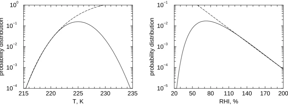
Fig. A1. Comparison between Gaussian temperature distribution and resulting quasi-exponential distribution of RHI (solid curves, left and right panel, respectively) with corresponding analytical solutions valid at low temperatures and high relative humidities (dashed curves) describing an exact asymptotic exponential decrease of the distribution of RHI.
with the parameterT¯ at which8(T ) reaches its maximum andω= ¯Sexp(−θ/T ).¯
Figure A1 (left panel) depicts the normally distributed temperatures 8n(T ) from Eq. (5) with To=225 K and
σ=2.5 K (solid curve) along with the distribution Eq. (A3) withC=1.85 andT¯=237 K (dashed curve). The right panel depicts the resulting distributions ofS from Eq. (10) with So=0.8 (solid curve; the same distribution is plotted as a
dashed red curve in Fig. 2) and from Eq. (A2) withS¯=0.2 (a value consistent with the MOZAIC data).
The agreement between the exact Gaussian distribution forT and the exact exponential distribution for S with our analytic solutions Eqs. (A3) and (A2) is very remarkable. We may argue that much larger deviations from an exact exponential fall-off than those shown in Fig. A1 cannot be discerned from atmospheric measurements of RHI, because typical experimental uncertainties of RHI are some ±5% or higher. Such deviations may be caused by additional variability due to adiabatic corrections and variations ofχ (which have been ignored in the analytic solution) or by low temperature tails of the distributions ofT that do not exactly follow a Gaussian distribution or Eq. (A3), including those arising from small-scale temperature fluctuations as exam-ined in Sect. 4.3.
Acknowledgements. We thank Klaus Gierens for comments on a draft version of this manuscript and Andrew Gettelman for a use-ful discussion. This research was conducted within the projects “Particles in the Upper Troposphere and Lower Stratosphere and Their Role in the Climate System” (PARTS) and ”Interhemispheric Differences in Cirrus Properties From Anthropogenic Emissions” (INCA), funded by the European Commission, and contributes to the project “Particles and Cirrus Clouds” (PAZI) supported by the Helmholtz-Gemeinschaft Deutscher Forschungszentren (HGF).
Topical Editor O. Boucher thanks two referees for their help in evaluating this paper.
References
Bacmeister, J. T., Eckermann, S. D., Tsias, A., Carslaw, K. S., and Peter, Th.: Mesoscale temperature fluctuations induced by a spectrum of gravity waves: A comparison of parameterizations and their impact on stratospheric microphysics, J. Atmos. Sci., 56, 1913–1924, 1999.
Fischer, H., de Reus, M., Traub, M., Williams, J., Lelieveld, J., de Gouw, J., Warneke, C., Schlager, H., Minikin, A., Scheele, R., and Siegmund, P.: Deep convective injection of boundary layer air into the lowermost stratosphere at midlatitudes, Atmos. Chem. Phys., 3, 739–745, 2003.
Gary, B.: Mesoscale temperature fluctuations: An overview, http: //reductionism.net.seanic.net/bgary.mtp2/isentrop/index.html, 2002.
Gettelman, A., Randel, W. J., Wu, F., and Massie, S. T.: Transport of water vapor in the tropical tropopause layer, Geophys. Res. Lett., 29, doi:10.1029/2001GL013818, 2002.
Gierens, K. M., Schumann, U., Smit, H. G. J., Helten, M., and Z¨angl, G.: Determination of humidity and temperature fluctua-tions based on MOZAIC data and parameterisation of persistent contrail coverage for general circulation models, Ann. Geophys-icae, 15, 1057–1066, 1997.
Gierens, K. M., Schumann, U., Helten, M., Smit, H., and Marenco, A.: A distribution law for relative humidity in the upper tro-posphere and lower stratosphere derived from three years of MOZAIC measurements, Ann. Geophysicae, 17, 1218–1226, 1999.
Gierens, K. M., and Brinkop, S.: A model for the horizontal ex-change between ice-supersaturated regions and their surround-ings, Theor. Appl. Climatol., 71, 129–140, 2002.
Haag, W., K¨archer, B., Str¨om, J., Minikin, A., Ovarlez, J., Lohmann, U., and Stohl, A.: Freezing thresholds and cirrus cloud formation mechanisms inferred from in situ measurements of rel-ative humidity, Atmos. Chem. Phys., 3, 1791–1806, 2003. Heymsfield, A. J., Miloshevich, L. M., Twohy, C., Sachse, G., and
2002.
Jeffreys, H., Theory of Probability, second edition, Oxford Univ. Press, 1948.
Jensen, E. J., Toon, O. B., Vay, S. A., Ovarlez, J., May, R., Bui, P., Twohy, C. H., Gandrud, B., Pueschel, R. F., and Schumann, U.: Prevalence of ice-supersaturated regions in the upper tropo-sphere: Implications for optically thin ice cloud formation, J. Geophys. Res., 106, 17 253–17 266, 2001.
K¨archer, B., and Solomon, S.: On the composition and optical ex-tinction of particles in the tropopause region, J. Geophys. Res., 104, 27 441–27 459, 1999.
K¨archer, B., and Str¨om, J.: The roles of dynamical variability and aerosols in cirrus cloud formation, Atmos. Chem. Phys., 3, 823– 838, 2003.
Koop, T., Luo, B. P., Tsias, A., and Peter, Th.: Water activity as the determinant for homogeneous ice nucleation in aqueous so-lutions, Nature, 406, 611–614, 2000.
Marti, J., and Mauersberger, K.: A survey and new measurements of ice vapor pressure at temperatures between 170 and 250 K, Geophys. Res. Lett., 20, 363–366, 1993.
Murphy, D. M., Kelly, K. K., Tuck, A. F., Proffitt, M. H., and Kinne, S.: Ice saturation at the tropopause observed from the ER-2 air-craft, Geophys. Res. Lett., 17, 353–356, 1990.
Ovarlez, J., van Velthoven, P., Sachse, G., Vay, S., Schlager, H., and Ovarlez, H.: Comparisons of water vapor measurements from POLINAT 2 with ECMWF analyses in high-humidity conditions, J. Geophys. Res., 105, 3737–3744, 2000.
Ovarlez, J., Gayet, J.-F., Gierens, K., Str¨om, J., Ovarlez, H., Auriol, F., Busen, R., and Schumann, U.: Water vapour measurements inside cirrus clouds in Northern and Southern hemispheres during INCA, Geophys. Res. Lett., 29, 1813, doi:10.1029/2001GL014440, 2002.
Peter, Th.: Microphysics and heterogeneous chemistry of polar stratospheric clouds, Annu. Rev. Phys. Chem., 48, 785–822, 1997.
Schlager, H., Schulte, P., and Volkert H.: Estimate of diffusion parameters of aircraft exhaust plumes near the tropopause from nitric oxide and turbulence measurements, J. Geophys. Res., 100, 14 147–14 162, 1995.
SPARC Assessment of Upper Tropospheric and Stratospheric Water Vapor, D. Kley and J. M. Russell III (Co-chairs), World Climate Research Program (WCRP), WCRP-113, World Meteorological Organization (WMO), WMO-TD No. 1043, Stratospheric Pro-cesses and Their Role in Climate (SPARC) Report No. 2, 233– 240, December, 2000.
Spichtinger, P., Gierens, K., and Read, W.: The statistical distri-bution law of relative humidity in the global tropopause region, Meteorol. Z., 11, 83–88, 2002.
Str¨om, J., Seifert, M., K¨archer, B., Minikin, A., Gayet, J.-F., Krejci, R., Petzold, A., Auriol, F., Haag, W., Busen, R., Schumann, U., and Hansson, H.-C.: Cirrus cloud occurrence as a function of am-bient relative humidity: A comparison of observations from the Southern and Northern Hemisphere midlatitudes obtained dur-ing the INCA experiment, Atmos. Chem. Phys., 3, 1807–1816, 2003.
Tabazadeh, A., Toon, O. B., Gary, J., Bacmeister, J. T., and Schoe-berl, M. R.: Observational constraints on the formation of type 1a polar stratospheric clouds, Geophys. Res. Lett., 23, 2109–2112, 1996.
Thornton, B. F., Toohey, D. W., Avallone, L. A., Harder, H., Mar-tinez, M., Simpas, J. B., Brune, W. H., and Avery, M. A.: In situ observations of ClO near the winter polar tropopause, J. Geo-phys. Res., 108, 8333, doi:10.1029/2002JD002839, 2003. Vay, S. A., Anderson, B. E., Jensen, E. J., Sachse, G. W., Ovarlez,