Nonlinear time series analysis of the fluctuations of the geomagnetic horizontal field

Annales

Geophysicae

Nonlinear time series analysis of the fluctuations of the geomagnetic

horizontal field

B. George1, G. Renuka1, K. Satheesh Kumar2, C. P. Anil Kumar3, and C. Venugopal4

1_{Department of Physics, University of Kerala, Kariavattom, Thiruvananthapuram, Kerala - 695 581, India} 2_{Department of Mathematics, St. John’s College, Anchal PO, Kerala - 691 306, India}

3_{School of Pure and Applied Physics, Mahatma Gandhi University, Priyadarshini Hills PO, Kottayam, Kerala - 686 560, India} 4_{Department of Physics, University of Asmara, PO Box 1220, Eritrea}

Received: 27 November 2000 – Revised: 2 May 2001 – Accepted: 28 June 2001

Abstract. A detailed nonlinear time series analysis of the hourly data of the geomagnetic horizontal intensityH mea-sured at Kodaikanal (10.2◦N; 77.5◦E; mag: dip 3.5◦N) has been carried out to investigate the dynamical behaviour of the fluctuations ofH. The recurrence plots, spatiotemporal entropy and the result of the surrogate data test show the de-terministic nature of the fluctuations, rejecting the hypothesis thatH belong to the family of linear stochastic signals. The low dimensional character of the dynamics is evident from the estimated value of the correlation dimension and the frac-tion of false neighbours calculated for various embedding di-mensions. The exponential decay of the power spectrum and the positive Lyapunov exponent indicate chaotic behaviour of the underlying dynamics ofH.This is also supported by the results of the comparison of the chaotic characteristics of the time series ofH with the pseudo-chaotic characteris-tics of coloured noise time series. We have also shown that the error involved in the short-term prediction of successive values ofH, using a simple but robust, zero-order nonlin-ear prediction method, increases exponentially. It has also been suggested that there exists the possibility of character-izing the geomagnetic fluctuations in terms of the invariants in chaos theory, such as Lyapunov exponents and correlation dimension. The results of the analysis could also have impli-cations in the development of a suitable model for the daily fluctuations of geomagnetic horizontal intensity.

Key words. Geomagnetism and paleomagnetism (time vari-ations, diurnal to secular) – History of geophysics (solar-planetary relationships) Magnetospheric physics (storms and substorms)

1 Introduction

The geomagnetic field pervades the region around the Earth, extending to several times of the radius of the Earth. Solar output, in terms of solar plasma and magnetic field, ejected Correspondence to: G. Renuka ([email protected])

out into the interplanetary medium contributes greatly to the perturbation in the geomagnetic field. Episodes of extra or-dinary fluctuations in Earth’s magnetic field were detected as storms in the mid 1800’s. The analysis of the fluctuations in the geomagnetic field has many practical applications in magnetic navigation, orientation control, geophysical explo-ration, etc. (Newitt, 1993; Kerridge, 1993; Gonzalez et al., 1994; Sutcliffe, 2000). The analysis of storm morphology has been undertaken by several authors. Different defini-tions of geomagnetic storms have been given by Gonzalez et al. (1994). According to the classical definition, a geo-magnetic storm occurs when the dailyApindex exceeds 29,

a minor storm occurs when 30 ≤ Ap < 50; a major storm

occurs when 50 ≤ Ap < 100 and a severe storm occurs

whenAp≥100 (Lundstedt, 1996).

A continuous recording of any of the components of the geomagnetic field typically exhibits two types of variations: a smooth, regular variation, known as Sq, and the solar quiet day variation, which arises as the magnetic signature of the E-region ionosphere current driven by a dynamo ac-tion (Campbell, 1989) and a rapid irregular fluctuaac-tion, re-ferred to as a geomagnetic disturbance or storm, the mag-nitude of which may be such that the regular Sq variation is swamped and thus, not easily discernible. Although the

-300 -200 -100 0 100 200 300 400

0 1000 2000 3000 4000 5000 6000 7000 8000

H (nT)

Time (hour) (a)

-300 -200 -100 0 100 200 300 400

-300 -200 -100 0 100 200 300 400

sn-5

sn (b)

Fig. 1. (a) Time series of the geomagnetic fieldH.(b) Delay

repre-sentation of the time series ofH.

decrease in H at low-latitudes, with an increasing Ap

in-dex during extremely quiet periods and suggested the effect is associated with the interaction of the solar wind on the magnetosphere. One of the objectives of investigation of the dynamical behaviour of the fluctuations of the geomagnetic field is to predict storms. Wang (1996) has applied fractal theory in a quantitative analysis of geomagnetic storms and has estimated the correlation dimension of the attractor for storm data from the Beijing observatory (40.0◦_{N, 116.2}◦_E). Nonlinear dynamic methods have been applied to mag-netospheric data in order to study the underlying dynamics (Sharma, 1995; Klimas et al., 1996). Studies using these methods have given results supporting the concept of mag-netospheric chaos (Vassiliadis et al., 1990, 1992; Robert et al., 1991; Shan et al., 1991; Pavlos et al., 1992, 1994, 1999a, b, c). However, several studies have given evidence against the hypothesis of magnetospheric chaos and indicate the sig-nificant role of the stochastic solar wind driver (Prichard and Price, 1993; Price et al., 1994; Takalo and Timonen, 1994, Prichard, 1994). Klimas et al. (1996) have given an excellent review of the studies on these aspects. The criticism about the magnetospheric chaos has been recently addressed in a series of papers by Pavlos et al. (1999a, b, c). They have

tested the null hypothesis that the observedAEindex signal is generated by a linear stochastic signal, possibly perturbed by a static nonlinear distortion. In the first paper (Pavlos et al., 1999a) of the series, they have used four distinct geomet-ric parameters derived from the slope of the correlation in-tegral as discriminating statistical procedures in order to test the null hypothesis of the nonlinear stochastic surrogate data, which have the same power spectrum and amplitude distri-bution as the original data. In the second paper (Pavlos et al., 1999b), dynamical characteristics, such as Lyapunov ex-ponents, nonlinear dynamic models and mutual information, were used to test the null hypothesis. The results of these tests suggest the rejection of the null hypothesis that theAE

index signal belongs to the family of stochastic signals un-dergoing a static nonlinear distortion, i.e. the results of these studies strongly support the hypothesis of nonlinearity and chaotic behaviour of the underlying dynamics of the magne-tospheric system. In continuation of these studies, they have introduced significant theoretical concepts about the magne-tospheric system and its dynamical interaction with the so-lar wind (Pavlos, 1999c). Based on the comparison of the observational behaviour of the magnetospheric system with the results of the analysis of the different types of stochastic and deterministic input-output systems, they have observed that the hypothesis of low-dimensional chaotic behaviour of the magnetospheric dynamics remains a possible and fruitful concept which must be developed further. Hence, we feel that the tools of nonlinear time series analysis can be used with confidence in order to obtain useful information about the internal deterministic component of a magnetospheric time series.

Our main objective in this work is to carry out a detailed nonlinear time-series analysis of the time series of the mea-surements of the geomagnetic horizontal fieldH. The data we used in this analysis represent the geomagnetic horizon-tal intensityH, measured during the year 1991 at a one hour interval at the Kodaikanal observatory and published by the Indian Institute of Geomagnetism, Bombay. The importance of this data is thatHvaries drastically during the year and in addition, we noted 33 storms, out of which five were severe. The time series ofHis plotted in Fig. 1a and its delay repre-sentation in Fig. 1b. The origin of the values ofH has been shifted to 39 000 nT.

2 Nonlinear time series analysis

time delay coordinates. Embedding theorems (Sauer et al., 1991) guarantee that for an appropriate delay depending on the data, at most 2d+1 delay coordinates are enough, when

d is the fractal dimension of the attractor. A time series is a sequence of scalar measurements of some quantity which depends on the current state of the system, taken at multiples of a fixed sampling time:

sn=s(y(n1t ))+ηn, (1)

whereηn is the measurement noise. A delay reconstruction

inmdimensions is then found by the vectorsyn, given by

yn=(sn−(m−1)v, sn−(m−2)v, . . . , sn−v, sn). (2)

The time difference in number of samplesvbetween adja-cent components of the delay is referred to as the lag or delay time. One of the problems of the nonlinear time-series anal-ysis is to find an optimal embedding dimensionm.However, for many practical purposes, the most important embedding parameter is the productmτ of the embedding dimensionm

and the delay timeτ, sincemτ is the time span represented by an embedding vector. A precise knowledge ofmis only required when we want to exploit determinism with minimal computational effort (Kantz and Schreiber, 1997). Neverthe-less, there are several indicators of an optimal embedding di-mensionm.One such indicator is the correlation dimension

D, defined by

D= lim

r→0 lnC(r)

lnr , (3)

whereC(r)is the correlation sum for radiusr, which reveals a scaling profile asC(r) ∼ rd forr → 0.The correlation sum depends on the embedding dimensionmof the recon-structed phase space and the length of the time seriesN as

C(r)= 2

N (N−1)

N X

i=1

N X j=i+1

2(r− kyi−yjk), (4)

where2is the Heaviside step function,2(a)=0 ifa ≤ 0 and2(a)=1 fora >0.The scaling exponentd increases withmand saturates to a final value of D for sufficiently large embedding dimensionmo. In most cases,momay be

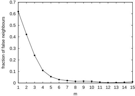
the smallest integer larger thanD(Ding et al., 1993). When the slopes d of the correlation integral for various embed-ding dimensions reveal a plateau at low values ofr and the plateau converges for increasingm, then there is strong ev-idence for a low-dimensionality of the underlying dynamics of the system. Calculation of the correlation dimension from the time series is easy, compared to the calculation of other dimensions and, in most cases, gives a good approximation to the actual dimension of the attractor. Another technique to estimate an optimal value ofmis to look for the closed false neighbors (FNN) in the phase space at a given value of m (Kennel et al., 1992). As the embedding dimension increases, the number of false neighbours decreases. Thus, one can detect the minimal embedding dimension which cor-responds to the minimum number of false neighbours. These

0 0.1 0.2 0.3 0.4 0.5 0.6 0.7

1 2 3 4 5 6 7 8 9 10 11 12 13 14 15

fraction of false neighbours

m

Fig. 2. The fraction of the closest false neighbours as a function of

the embedding dimensionmfor the time series.

techniques give the optimal number of independent variables required to reconstruct the underlying attractor of the dynam-ical system from the time series. Most of the significant char-acteristics of the original phase space are carried over to the reconstructed phase space for the sufficient large embedding dimension obtained in the above discussed methods. Math-ematically speaking, the geometrical characteristics of the original phase space are topologically equivalent to its mir-ror dynamical flow in the reconstructed phase space. Conse-quently, it is possible to make both qualitative and quantita-tive statements about the system based on the time series by using the tools of a nonlinear time-series analysis. Thus, it is relevant to carry out a detailed, nonlinear time-series analy-sis of the fluctuations of the geomagnetic horizontal intensity

H.The results of the analysis are discussed in the following section.

3 Results and discussion

We started the analysis by estimating an optimal value of the embedding dimensionm, using the method of the closest false neighbours. The fraction of the closest false neighbours as a function of the embedding dimension is plotted in Fig. 2. It is evident from the figure that the fraction of false neigh-bours decreases drastically after the first few values ofm.In order to establish the low dimensionality of the attractor, we have also calculated the correlation dimension.

Attractors of dissipative chaotic systems generally have very complex geometry and hence, are called the strange at-tractors. One of the parameters that characterizes an attractor is its dimension, which can be regarded as a measure of the amount of information necessary to specify the position of a point on the attractor within a given accuracy. The correla-tion dimension is one such parameter which depends on the spatial correlation of points on the attractor.

0 50 100 150 200 250 300

0 20 40 60 80 100 120

r

Dt

Fig. 3. The space-time separation plot for the time series ofH. Initially, the curves increase quickly and later, the stable diurnal oscillations repeat.

attractor (Theiler, 1991). In order to remove this spurious ef-fect, the temporally correlated points are excluded from the pair counting in the correlation sum, i.e. the sum in Eq. 4 is restricted to pairs of points whose time indices differ by at leastω, called the Theiler window (Theiler, 1991). Heg-ger et al. (1999) have suggested that the value ofωshould be chosen generously. The space-time separation plot intro-duced by Provenzale et al. (1992) provides a good means of determining a sufficient value ofω(Hegger et al., 1999). In the presence of temporal correlations, the probability that a given pair of points has a distance smaller thanrdepends on bothr and also on the time1tbetween the two points. In a space-time separation plot, the number of pairs is plotted as a function of two variables, the time separation1t and the spatial distancer(Hegger et al., 1999).

The space-time separation plot of the geomagnetic hori-zontal field H is given in Fig. 3. The diurnal variability is dominant in this system and is reflected in Fig. 3. The temporal correlation is evident within the first 12 time steps where the lines increase consistently. However, the oscilla-tions saturate after a few cycles. To be safe, we have cho-sen the minimum correlation time to be 100. However, we have varied the value of the Theiler parameterω from 100 to 1000 for the calculation of the correlation dimension, but there was no significant difference. The value of the correla-tion dimension calculated is 3.70±0.04 which corresponds to a good plateau, as shown in Fig. 4. This fractional cor-relation dimension indicates the existence of a strange, low dimensional attractor.

We then analyzed the deterministic nature of the time se-ries. This is important since a finite time series with a broad band power spectrum may be a realization of a stochas-tic process governed by an autoregressive moving average model or of a low dimensional deterministic chaotic pro-cess (Eckman and Ruelle, 1985). It has also been noted that some geometrical and dynamical characteristics (low corre-lation dimension and positive Lyapunov exponent, etc.) of

0 2 4 6 8 10 12 14 16 18

0 50 100 150 200 250 300 350 400

d(r)

r (a)

1e-07 1e-06 1e-05 0.0001 0.001 0.01 0.1 1

10 100 1000

C(r)

r (b)

Fig. 4. (a) Local slopes of the logarithm of the correlation sum

for the geomagnetic horizontal intensityH form = 12, τ = 10 andω = 100.The correlation dimensionD = 3.70±0.04.(b)

The correlation sumC(r)ofH form=8,9, . . . ,20, τ = 10 and ω=100.

the low dimensional chaotic dynamics can also be observed from a particular linear stochastic process. We employed the method of surrogate data and also the Recurrence Plots (Eck-man et al., 1987) to distinguish between linear stochastic and deterministic dynamics.

The method of surrogate data has been reported to be a successful tool of choice for the identification of a nonlin-ear deterministic structure in an experimental data (Mitschke and D¨ammig, 1993). It is specifically devised to contrast a data set under study with data that are similar with respect to linear correlations, but otherwise purely random. Accord-ing to this method, the geometrical and dynamical charac-teristics of the data under study is compared with those of stochastic signals which have the same Fourier amplitudes and the same distribution of values. If the behaviour of the original data and the surrogate data are significantly differ-ent in such characteristics, then it may be safely concluded that the process under study cannot be described by a sta-tionary, linear Gaussian stochastic model. The significance of the difference of the local slopes of the correlation sums can be defined as

S= µ−µorig

σ , (5)

whereµis the mean value of the local slopes of the correla-tion sums of different surrogates, andσ is their standard de-viation (Mitschke and D¨ammig, 1993; Pavlos et al., 1999a). For our analysis, a group of 40 surrogates of the time se-riesH were generated based on the algorithm of Schreiber and Schmitz (1996). The plot of the local slopes of the cor-relation sums of the surrogates, along with that of H as a function of ln(r), is given Fig. 5a. Figure 5b gives its mean value and the standard deviation (S. D.). For the region where

S > 2, we can reject with a confidence above 95% the null

0 2 4 6 8 10 12

30 60 120

Local slopes

Ln(r) (a)

Surrogate data H

0 1 2 3 4 5 6 7 8 9 10 11

30 60 120

Local slopes

Ln(r) (b)

H mean value of the surrogates mean + S.D.

0 1 2 3 4 5 6 7 8

30 60 120

S

Ln(r) (c)

Fig. 5. (a) The local slopes of the correlation sums of the surrogates

as function of ln(r)form=12, τ=10 andω=100.(b) The mean

values of the local slopes of the surrogates with standard deviation form=12, τ =10 andω=100.(c) Plot of the significance of the

differenceSversus ln(r).

stochastic process (Pavlos et al., 1999a). As shown in Fig. 5c, the significance of the differenceSreaches above 7 for small values ofr, and remains above 2 for a larger interval of small

rvalues.

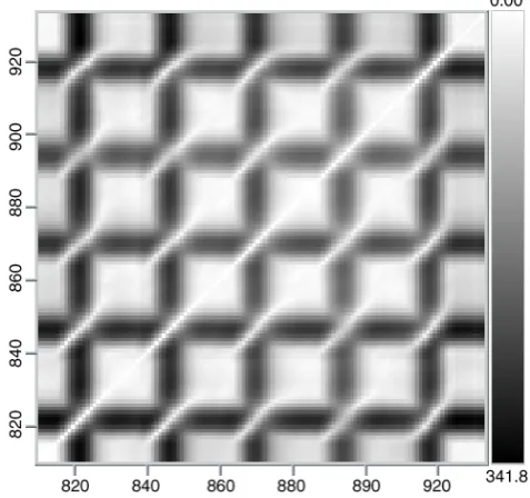
We have also used the recurrence plot of the time series ofH to identify the structure in the data. Recurrence plots

Fig. 6. The recurrence plot of the time series ofH.

are useful to graphically detect hidden patterns and structural changes in data or to see similarities in patterns across the time series under study (Eckman et al., 1987). Once the dynamical system is reconstructed by means of delay co-ordinates, the distances between all pairs of vectorsyi and

yj are computed and various colour-codes are assigned to

different distances. In a two-dimensional recurrence plot, a colour-code at position(i, j )specifies the distances between the vectorsyi andyj.For random signals, a uniform

distri-bution of colours over the entire plane is obtained, whereas for deterministic signals, the recurrence plot contains beau-tiful structures. The recurrence plot in the grey scale of the time series in this study is given in Fig. 6, which provides evidence of the determinism in the data.

In addition to these techniques, we have also computed the spatiotemporal entropy. This quantity compares the distribu-tion of distances between all pairs of vectors in the recon-structed phase space with distances between different orbits evolving in time. For random signals, the value of the spa-tiotemporal entropy will be 100%, whereas for deterministic signals the value lies in between 0 and 100. In our case the value computed was close to zero, showing perfect structure in the data. From the above observations, we can safely con-clude that the geomagnetic horizontal intensityH does not belong to the family of linear stochastic signals. Thus, the fluctuations observed in the time series ofHare due to a low dimensional deterministic process.

It has been observed that a time series of coloured noise can also exhibit a power law power spectrumω−α which is typical of a chaotic time series. The correlation dimensionD

-0.2 0 0.2 0.4 0.6 0.8 1

0 10 20 30 40 50 60 70

Autocorrelation Coefficient

Time (days)

Colored Noise H

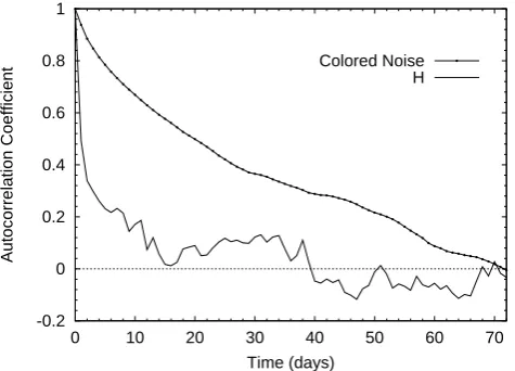
Fig. 7. The autocorrelation coefficient of the time series ofH and that of the coloured noise with the same correlation dimensionD=

3.7.

coloured noise can be generated by letting

x(j )=

N/2

X k=1

Ckcos(2πj k/N−φk)forj =1,2, . . . , N, (6)

where the coefficientsCk, related to the power law power

spectrumP (k)∝k−αby

Ck =

P (k)2π

N

1/2

(7)

and the phasesφk, are randomly distributed in[0,2π].

Pav-los et al. (1992) have discussed the methods to compare the chaotic characteristics of an experimental time series with the pseudo-chaotic characteristics of a coloured noise time series.

The autocorrelation coefficients of H and that of the coloured noise time series with same fractal dimension is plotted in Fig. 7. For small lag times, the autocorrelation coefficient ofH drops quickly, whereas that of the coloured noise decreases very slowly. There is also a significant dif-ference in the decorrelation time. The autocorrelation coef-ficient ofH drops abruptly by days 14 and 15 and reaches zero by day 40. However, the coloured noise takes about 72 days to become decorrelated.

The randomization of the phases of a deterministic chaotic signal can destroy its low dimensional chaotic profile. How-ever, this profile of a coloured noise time series remains in-variant under the phase randomization (Pavlos et al., 1992). We have compared the low dimensional profile of the time series ofHto that of the time series obtained by the random-ization of phases of the time series ofH.The phase random-ized time series ofH was obtained from the Fourier series representation ofH

x(ti)=

X k

Ckcos(ωkti+φk), (8)

0 2 4 6 8 10 12 14 16

0 50 100 150 200 250 300

d(r)

r (a)

0 4 8 12 16 20

0 100 200 300

d(r)

r (b)

Fig. 8. (a) Plot of the local slopes of the logarithm of the

corre-lation sums of the phase randomized time series ofH form =

1,2, . . . ,20, τ = 10 andω =100.(b) The same for the original

times series ofH form=12,13, . . . ,20, τ=10 andω=100.

where the phasesφkare distributed randomly on the interval

[0, 2π]. Figure 8a shows the local slopes of the logarithm of the correlation sums of the phase randomized time series of

Hand Fig. 8b shows that of the original time series ofH. It is evident from these figures that the low dimensional chaotic profile is destroyed by the phase randomization.

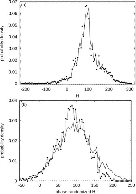
We then compared the stationarity of these two times se-ries. The fractional Brownian motions with coloured noise profiles can have a low dimensional character, but they are not stationary signals unlike motions on a strange attractor (Pavlos et al., 1992). For a stationary process, the probabil-ity densprobabil-ity in phase space must be invariant with time. The probability density of the time series ofH is calculated by dividing the range of the values ofH into short intervals and counting the values ofH which fall in those intervals. Fig-ure 9a shows the probability density calculated for the origi-nal times seriesH.The solid line shows the probability den-sity calculated for the entire time series and the filled circles corresponds to the first half of the time series. The coinci-dence is very clear in this figure. Figure 9b shows the prob-ability calculated for the phase randomized time series ofH.

In this figure, the solid line corresponds to the entire time se-ries and the dashed line with filled circles corresponds to the first half of the series. The coincidence in this figure is very low and this reveals the nonstationary character of the phase randomized signal. These results also show the deterministic character of the time series ofH.

The power spectrum of the time series ofH shows expo-nential decay which excludes the possibility of random be-haviour and thus, indicates the chaotic bebe-haviour of the time series (Fig. 10). It is also evident from Fig. 10 that there are five distinct peaks and they corresponds toAp =300 nt,

300 nt, 179 nt, 236 nt, 300 nt, respectively, and hence, repre-sent severe storms.

0 0.01 0.02 0.03 0.04 0.05 0.06 0.07

-200 -100 0 100 200 300

probability density

H (a)

0 0.01 0.02 0.03 0.04

-50 0 50 100 150 200 250

probability density

phase randomized H (b)

Fig. 9. (a) The probability density function of the original time

series ofHbased on the entire time series (solid line) and on the first half of the series (filled circles). (b) The probability density function of the phase randomized time series ofH based on the entire time series (solid line) and on the first half of the series (dashed line with filled circles).

the calculation of Lyapunov characteristic exponents which, if positive, by definition, are the most striking evidence of chaos (Kantz, 1994). The first algorithm to a compute Lya-punov exponent for a time series was introduced by Wolf et al. (1985). One of the drawbacks of the algorithm of Wolf et al. (1985) is the strong dependence of the embedding di-mension (Kantz, 1994). In this work, we used the algorithm developed by Kantz (1994) to calculate the maximum Lya-punov exponent. According to this method, one has to com-pute

S(1n)= 1

N

N X n0=1

ln

1 |U(yno)|

X

ynU(yno)

|sno+1n−sn+1n|

!

(9)

for a pointyno of the time series in the embedding space, whereU(yno)is the neighborhood of yno with diameterr. This is repeated for many values ofn0so that the fluctuations

0.01 0.1 1 10 100 1000 10000

0 0.05 0.1 0.15 0.2 0.25 0.3 0.35 0.4 0.45

Power

Frequency (0.001)

Fig. 10. The power spectrum of the times series withw =0.001. The first part of the spectrum corresponds to an abrupt decay and the second part corresponds to a slow decay, as shown by the dis-continuous lines.

-5 -4.5 -4 -3.5 -3 -2.5 -2 -1.5 -1

0 5 10 15 20 25 30 35 40 45

exp(S)

Dn

Fig. 11. The curve ofeS(1n)for the embedding dimensionm=12. The slope of the dashed line is 0.25±0.006 and it is the maximum Lyapunov exponent of the time series ofH.

of the effective expansion rates are averaged out. For an in-termediate range of values of1n,S(1n)increases linearly with slopeλ, which is our estimate of the maximal Lyapunov exponent. In this work, we have repeated the computation

of S(1n)for different values of the embedding dimension

mand the diameter of the neighbourhoodr. The maximum Lyapunov exponent was estimated to beλ = 0.25±0.006 for the time series ofH (Fig. 11).

condi-60 80 100 120 140 160 180 200

1 2 3 4 5 6 7 8 9 10

0.37 0.38 0.39 0.4 0.41 0.42 0.43

Geomagnetic field H (nT)

Normalized error

Time (hr) Actual values Predicted values Normalized error

Fig. 12. The predicted (using the zero-order nonlinear prediction

method) values of the times series ofH is plotted along with the actual values and the normalized error.

tions and the Lyapunov exponent. The prediction of subse-quent values of the times series of H, using a simple but robust zero-order nonlinear prediction method (Kantz and Schreiber, 1997), is given in Fig. 12, along with the nor-malized root mean-square errors. It may be noted that the root mean-square errors increases exponentially. This could be seen as further evidence of the deterministic nature of the fluctuations and also of the underlying chaotic behaviour.

4 Conclusion

In this work, an investigation of the fluctuations of the time series of the geomagnetic horizontal intensityH, using the tools of nonlinear time series analysis, has been carried out. The recurrence plots and the results of surrogate data method, in addition to the estimate of spatiotemporal entropy, shows the deterministic nature of the data. We have also compared the chaotic characteristics of the time series ofH with the pseudo-chaotic characteristics of coloured noise time series generated by the phase randomization of the original time series. The results of the comparison also reveal the deter-minism in the data. In addition to the estimated value of the correlation dimension, the analysis of the data, according to the method of the closest false neighbours, also shows the low dimensional character of the underlying dynamics. The positive value of the maximum Lyapunov exponent and the exponential decay of the power spectrum shows the chaotic behaviour of the dynamics. Thus, the physical process under-lying the fluctuations ofHis deterministic, low dimensional and chaotic. We have also shown that the error involved in the short-term prediction of the successive values ofH, using a simple but robust, zero-order nonlinear prediction method (Kantz and Schreiber, 1997), increases exponentially and this indicates the sensitive dependence on the initial conditions. Wang (1996) has proposed that a combination of the corre-lation dimension of the attractor of the storm data and the magnetic indexkcould perhaps better describe the degree of

solar disturbance than the single parameterk.We have es-timated both the geometric and dynamical invariants of the attractor for the geomagnetic horizontal intensity, such as the correlation dimension and Lyapunov exponents, and we feel that it would be more advantageous to include the dynamical invariants, such as Lyapunov exponents, into this combina-tion to describe the solar disturbance. In general, the quan-tities involved in chaos theory could be used to characterize the fluctuations of the geomagnetic intensity and hence, to describe the associated phenomena more accurately. The re-sults of the analysis could also have implications in the de-velopment of a suitable model for the daily fluctuations of geomagnetic horizontal intensity.

Acknowledgements. The authors are grateful to the referees of this paper for their constructive comments which helped to improve the presentation of this paper substantially. One of the authors (K. S.) thanks T. R. Ramamohan, Regional Research Laboratory (CSIR), Thiruvananthapuram for stimulating discussions.

Another one of the authors (B. G.) wishes to thank C. V. Deva-sia, Space Research Laboratory, VSSC, Thiruvananthapuram for his helpful suggestions.

Topical Editor M. Lester thanks N. Watkins and A. Klimas for their help in evaluating this paper.

References

Bhargava, B. N. and Subramanyan, R. V.: Geomagnetic distur-bances associated with equatorial electrojet, J. Atmos. and Terr. Phys., 26, 879–888, 1964.

Bhargava, B. N. and Yacob, A.: Solar cycle response in the hori-zontal force of the earth’s magnetic field, J. Geomagn. and Geo electr., 21 385–397, 1969.

Campbell, W. H.: The regular geomagnetic field variations during quiet solar conditions, in: Geomagnetism, Vol. 3, (Ed) Jacobs, J. A., Academic Press, London, 1989.

Ding, M., Grebogi, C., Ott, E., Sauber, T., and York, J. A.: Estimat-ing correlation from a chaotic time series: when does a plateau onset occur?, Physica D, 60, 404–424, 1993.

Eckman, J. P. and Ruelle, D.: Ergodic theory of chaos and strange attractors, Rev. Mod. Phys., 57, 617–628, 1985.

Eckman, J. P., Kamphorst, S. O., and Ruelle, D.: Recurrence plots of dynamical systems, Europhys. Lett., 4, 973–977, 1987. Gonzalez, W. D., Joselyn, J. A., Kamide, Y., Kroehl, H. W.,

Ros-toker, G., Tsurutani, B. T., and Vasyliunas, V. M.: What is a geomagnetic storm?, J. Geophys. Res., 99, 5771–5792, 1994. Grassberger, P. and Procaccia, I.: Measuring the strangeness of

strange attractor, Physica D, 9, 189–208, 1983.

Hegger, R., Kantz, H., and Schreiber, T.: Practical implimentation of nonlinear time series: the TISEAN package, chaos, 9, 413– 435, 1999.

Hibberd, F. H.: Day-to-day variability of theSqgeomagnetic field variation, Aust. J. Phys., 34, 81–90, 1981.

Joselyn, J. A., Kamide, Y., Kroehl, H. W., Rostoker, G., Tsurutani, B. T., and Vasyliunas, V. M.: What is a geomagnetic storm?, J. Geophys. Res., 99, 5771–5792, 1994.

Kantz, H. and Schreiber, T.: Nonlinear time series analysis, Cam-bridge University Press, CamCam-bridge, 1997.

Kennel, M. B., Brown, R., and Abarbanel, H. D. I.: Determining minimum embedding dimension using a geometrical construc-tion, Phys. Rev. A., 45, 3403–3411, 1992.

Kerridge, D. J.: Applications of geomagnetism in the oil industry, Paper 05.04.02 presented at the 7th Scientific Assembly IAGA, Buenos Aires, 1993.

Klimas, A. J., Vassiliadis, D., Baker, D. N., and Roberts, D. A.: The organized nonlinear dynamics of the magnetosphere, J. Geophys. Res., 101, 13 089–13 113, 1996.

Lundstedt, H.: Solar origin of geomagnetic storms and predictions, J. Atmos. Terr. Phys., 58, 821–830, 1996.

Mitschke, F. and D¨ammig, M.: Chaos versus noise in experimental data, in: Complexity and chaos, (Eds) Abraham, N. B., Albano, A. M., Passamante, A., Rapp, P. E., and Gilmore, R., World Sci-entific, Singapore, 1993.

Newitt, L. R.: Practical needs of users of magnetic declination infor-mation, Paper 05.09.07 presented at the 7th Scientific Assembly IAGA, Buenos Aires, 1993.

Osborne, A. R. and Provenzale, A.: Finite correlation dimension for stochastic systems with power-law spectra, Physica D, 35, 357– 381, 1989.

Parkinson, W. D.: Introduction to geomagnetism, Scottish Aca-demic Press, Edinburgh, 1983.

Pavlos, G. P., Athanasiu, M. A., Diamantidis, D., Rigas, A. G., and Sarris, E. T.: Nonlinear analysis of magnetospheric data Part I. Geometric characteristic of theAEindex time series and com-parison with nonlinear surrogate data, Nonlin. Proc. Geophys., 6, 51–65, 1999a.

Pavlos, G. P., Athanasiu, M. A., Diamantidis, D., Rigas, A. G., and Sarris, E. T.: Nonlinear analysis of magnetospheric data Part II. Dynamical characteristic of theAEindex time series and com-parison with nonlinear surrogate data, Nonlin. Proc. Geophys., 6, 79–98, 1999b.

Pavlos, G. P., Athanasiu, M. A., Diamantidis, D., Rigas, A. G., and Sarris, E. T.: Comments and new results about the magne-tospheric chaos hypothesis, Nonlin. Proc. Geophys., 6, 99–127, 1999c.

Pavlos, G. P., Diamadidis, D., Adamopoulos, A., Rigas, A. G., Daglis, I. A., and Sarris, E. T.: Chaos and magnetospheric dy-namics, Nonlin. Proc. Geophys., 1, 124–135, 1994.

Pavlos, G. P., Kyriakov, G. A., Rigas, A. G., Liatsis, P. I., Trochout-sos, P. C., and Tsonis, A. A.: Evidence for strange attractor struc-tures in space plasmas, Ann. Geophysicae, 10, 309–322, 1992. Price, C. P., Prichard, D. J., and Bischoff, J. E.: Nonlinear

input-output analysis of the auroral electrojet index, J. Geophys. Res., 99, 13 227–13 238, 1994.

Prichard, D. J. and Price, C. P.: Is theAEindex the result of

non-linear dynamics?, Geophys. Res. Lett., 20, 2817–2820, 1993. Prichard, D. J.: Short comment for magnetospheric chaos,

Nonlin-ear Proc. Geophys., 20, 771–774, 1994.

Provenzale, A., Smith, L. A., Vio, R., and Murante, G.: Distin-guishing between low-dimensional dynamics and randomness in measured time series, Physica D, 58, 31–49, 1992.

Roberts, D. A., Baker, D. N., Klimas, A. J., and Bargatze, L. F.: Indications of low dimensionality in magnetosphere dynamics, Geophys. Res. Lett., 18, 151–154, 1991.

Sauer, T., Yorke, J. A., and Casdagli, M.: Embedology, J. Stat. Phys., 65, 579–616, 1991.

Schreiber, T. and Schmitz, A.: Improved surrogate data for nonlin-earity tests, Phys. Rev. Lett., 77, 635–638, 1996.

Shan, H., Hansen, P., Goertz, C. K., and Smith, K. A.: Chaotic appearance of the ae index, Geophys. Res. Lett., 18, 147–150, 1991.

Sharma, A. S.: Assessing the nonlinear behaviour of the magne-tosphere: Its dimension is low, its predictability is high, (US National Report to IUGG, 1991-1994), Rev. Geophys., 33, 645– 650,(Supp), 1995.

Sugiura, M. and Chapman, S.: The average morphology of geomag-netic storms with sudden commencement, Abband. Akad. Wiss. Goettingen, Math. Physik. KI Sonderh, 4, 3–53, 1960.

Sutcliffe, P. R.: The development of a regional geomagnetic daily variation model using neural networks, Ann. Geophysicae, 18, 120–128, 2000.

Takalo, J. and Timonen, J.: Properties of ae data and bicolored noise, J. Geophys. Res., 99, 13 239–13 249, 1994.

Theiler, J.: Some comments on the correlation dimension of 1/fα noise, Phys. Lett. A, 155, 480–493, 1991.

Vassiliadis, D., Sharma, A. S., and Papadopoulos, K.: Time se-ries analysis of magnetospheric activity using nonlinear dynam-ical methods, in: Chaotic Dynamics: Theory and Practice, (Ed) Bountis, A., Plenum, New York, 1992.

Vassiliadis, D., Sharma, A. S., Eastman, T. E., and Papadopoulos, K.: Low-dimensonal chaos in magnetospheric activity fromAE time series, Geophys. Res. Lett., 17, 1841–1844, 1990.

Vestine, E. H., Laporte, L., Lange, I., and Scott, W. E.: The ge-omagnetic field – its description and analysis, Publi. No. 580, Carnegie Institution of Washington, Washington, 1947. Wang, T.: Fractals and magnetic storm, Ann. Geophysicae, 14,

888–892, 1996.

Wolf, A., Swift, J. B., Swinney, H. L., and Vastano, J. A.: Deter-mining Lyapunov exponents from a time series, Physica D, 16, 285–317, 1985.