publisher policies. Please scroll down to view the document
itself. Please refer to the repository record for this item and our
policy information available from the repository home page for
further information.
To see the final version of this paper please visit the publisher’s website.
Access to the published version may require a subscription.
Author(s): Adelman, James S and Brown, Gordon D. A.
Article Title: Modeling lexical decision: The form of frequency and
diversity effects.
Year of publication: 2008
Link to published version:http://dx.doi.org/
10.1037/0033-295X.115.1.214
decision: The form of frequency and diversity effects.
and
Postscript: Deviations from the predictions of serial search.
DOI:
10.1037/0033-295X.115.1.214
In press,
Psychological Review
, as at October 24, 2007.
This article may not exactly replicate the final version
published in the APA journal. It is not the copy of
record.
Running head: MODELING LEXICAL DECISION
Modeling Lexical Decision: The Form of Frequency and Diversity Effects
James S. Adelman and Gordon D. A. Brown
University of Warwick
Corresponding Author:
James S. Adelman
Department of Psychology,
University of Warwick,
Gibbet Hill Road,
COVENTRY,
CV4 7AL,
UK.
Telephone: +44 (0) 24 7615 0233
Abstract
What is the root cause of word frequency effects on lexical decision times? Murray and
Forster (2004) argued that such effects are linear in rank frequency, consistent with a
serial search model of lexical access. This paper (i) describes a method of testing models
of such effects that takes into account the possibility of parametric overfitting; (ii)
illustrates the effect of corpus choice on estimates of rank frequency; (iii) gives derivations
of nine functional forms as predictions of models of lexical decision; (iv) details the
assessment of these models and the rank model against existing data regarding the
functional form of frequency effects; and (v) reports further assessments using contextual
diversity, a factor confounded with word frequency. The relationship between the
occurrence distribution of words and lexical decision latencies to those words does not
appear compatible with the rank hypothesis, undermining the case for serial search
models of lexical access. Three transformations of contextual diversity based on extensions
Modeling Lexical Decision: The Form of Frequency and
Diversity Effects
The effect of word frequency on lexical processes is both ubiquitous and large. It is
evident in a wide range of both tasks (e.g., lexical decision, word naming, picture naming
and memorial tasks) and measures (especially response times and eye fixation times, but
also errors in the aforementioned tasks). It therefore seems reasonable to require models
of lexical tasks to account not only for the existence of frequency effects, but also for their
form. However, few existing models provide such an account. Murray and Forster (2004)
took up the challenge in the context of lexical decision times. Specifically, they showed
that their bin model, a frequency-ordered serial-search model of lexical access, predicts
that lexical decision times will be determined by the rank ordering of word frequency. In
comparisons between rank and logarithmic transformations, they argued that just this
pattern could be seen in the data, and (inter alia) interpreted this result as evidence for
serial search models.
As Murray and Forster (2004) made clear, one advantage of a clear theoretical
framework, such as their serial search model, is that it gives a principled prediction of the
functional form of frequency effects. According to Murray and Forster’s bin model, tasks
such as lexical decision require serial search of frequency-ordered lists. The expected
ranked position of a word in any list is a linear function of the word’s rank frequency,
leading to the prediction that expected search time will be linear in rank word frequency.
We agree with Murray and Forster that future progress will require the derivation and test
of specific predictions of fully explicated models such as the one described in their paper.
In particular, the evaluation of whether the ranked frequency of a word, rather than some
other (e.g., logarithmic, power, or exponential) transformation of frequency, predicts
lexical decision time would appear to have wide implications for quite general classes of
In this paper we consider several different classes of model architecture and derive
their specific predictions regarding the functional form of the word frequency effect (e.g.,
logarithmic, power and exponential from Bayesian, instance and contextual cue models
respectively). This allows us to evaluate different classes of model against several large
data sets. In particular, we explore some of the specific claims made by Murray and
Forster (2004) and question their conclusions regarding serial search models, before
turning to a more general survey of predictions regarding lexical decision latencies.
The plan of the paper is as follows. First, we examine Murray and Forster’s
dismissal (on the grounds of complexity) of the power transformation. We show that
additional tests on Murray and Forster’s own data suggest the superior fit of the power
transformation is not solely due to its propensity to overfit due to complexity. Second, we
argue (contrary to Murray and Forster’s assumption) that high correlations in frequency
among corpora do not guarantee accurate assessment of models based on rank word
frequency, suggesting the use of alternatives to the Kuˇcera and Francis (1967) word
frequency counts. In the third part of the paper, we derive predictions concerning the
functional form of word frequency effects from several different classes of model. In the
fourth part of the paper, we test these predictions regarding frequency effects with large
data sets and find evidence against a number of models. Finally, we argue that it is not
word frequency but rather the correlated factor of contextual diversity that determines
latency of access (McDonald & Shillcock, 2001; Adelman, Brown, & Quesada, 2006), and
conduct similar analyses with this variable. Overall, the additional analyses that we
report narrow the model types that can be considered compatible with existing data.
The evidence adduced by Murray and Forster (2004) for their model was based on
three new lexical decision experiments and on analyses of a subset of the data from a
mega-study by Balota, Cortese, and Pilotti (1999), using only the Kuˇcera and Francis
rank frequency over log frequency) was obtained for the Balota et al. (1999) data. Murray
and Forster (2004) used only lexical decision data to support their claims regarding lexical
access; we also consider only data from this task. Additional assumptions allowed an
extended version of the bin model to account for error rates (and error response times),
but the signature effect of such a model is a linear relationship between rank frequency
and (correct) lexical decision times, so any case against the model is both sufficient and
strongest if it is based on the response times. In addition, a focus on latencies rather than
error rates allows straightforward derivation of predictions from other classes of model,
and more accurate assessment of such predictions (because variance in error rates is high,
especially at the item level).
The Methodology of Comparing Fits of Frequency
Transformations
We first consider two methodological aspects of the Murray and Forster’s (2004)
assessment of transformations of frequency. These give the motivation for some of our
additional analyses.
Comparing Rank and Power Law Fits
Murray and Forster (2004) found that a power law transformation of frequency gave
a higher R2 on their (Experiment 1 and 2) data than did the rank of frequency. However,
they suggested that this result might have been an artifact arising from the additional
parameter of the power function. They supported this claim by simulations, the results of
which illustrated the fact thatR2 values can misleadingly favor a two-parameter power
function over a one-parameter linear function1.
This observation does not itself, however, indicate that the power law functional
form should be dismissed. It is important to know whether the observed R2 advantage for
larger than expected, as only the latter gives evidence against the simpler function. To
discover this, one can instead simulate many sets of data under the hypothesis that the
rank function generates response times in the task, in order to estimate the true
distribution of the power lawR2 (or any other statistic) under the rank hypothesis, and
then test whether the observed value falls in the tail of this distribution. In order to
generate response times under the rank (or any other) hypothesis, it is necessary to make
assumptions about the distribution of response times, because typically models predict
central tendency (in this case mean lexical decision time), but not the dispersion around
that central tendency. When a hypothesis is instantiated by using the empirical
(observed) distribution to estimate the distribution of the population under that
hypothesis, and the distribution of a statistic is examined under repeated resampling
(with replacement, and especially, but not necessarily, by simulation), this is known as a
bootstrap (Efron & Tibshirani, 1993).
Within the data we used here, the predictors, including frequency (however
transformed), are effectively fixed factors2. The appropriate procedure is then as follows.
One first fits the model under test (H0). Estimates are thereby obtained of the model’s
parameters, and of the distribution of errors in prediction (i.e., residuals). The observed
error distribution estimate is then used3 to generate simulated data around the
predictions of the model with the estimated parameters. This step is repeated many times
to produce several (B) bootstrap ‘replications’ of the experiment of interest. For each of
these, some statistic (T) of interest (for which higher values indicate moreH0 misfit) has
an estimate (t∗
i) calculated. Theset∗i values form an estimate of the overall distribution of
this statistic, which can be compared with its observed value (t) from the genuine
experiment. The size of the tail this cuts off (ˆp= #(t∗ > t)/B forT, where low ˆpvalues
are evidence against H0) can be used for a (usually one-tailed) null-hypothesis significance
discuss in this paper use the fit of some other model (Ha) as a component of the statistic
T (most simply, theR2 forH
a) so that evidence againstH0 is based onsystematic deviations from its predictions.
In our first illustrative analysis, we conducted simulations with the rank model as
H0 and examined theR2 of a power-law based model acting asH
a. (The derivation of
such a model with the exponent as a free parameter is given later in the paper.) Figure 1
shows the estimated distribution of a power function’sR2 (this acting as T), when rank
frequency generated the simulated data, with the simulation constructed on the basis of
the condition means from Murray and Forster’s (2004) Experiment 1. The mean was
90.3%, similar to the value obtained by Murray and Forster in their higher variance set of
simulations, and higher than the baseline (88.4%) for the fit of rank. This result is
consistent with the assertion that the R2 estimate is very biased. The observedR2 for the
power law functional form was 92.1%. This value did not fall in the 5% tail of the
distribution simulated under the rank hypothesis; in fact, ˆp=.324. However, whether the
R2 of the power function is surprisingly high (given the rank hypothesis is H
0) is better
considered by comparing it to the baselineR2 of the rank function, and asking whether
thedifference is surprisingly high. This procedure ameliorates the influence of
idiosyncratic properties of the sample. In many of the runs of the simulation (or indeed
actual replications of the experiment) where the powerR2 is high, the rankR2 will also be
high, as the predictions of the two models are in many cases very similar. For instance,
both will obtain their better fits when the frequency to response time relationship is
monotonic. Failing to take account of this relationship between the two values ofR2 being
compared therefore reduces the power of the test, just as using a between-subjectst-test
loses power when a within-subjects t-test is appropriate. Thus, some paired comparison is
necessary. The simplest such method, illustrated in Figure 2, uses the difference score of
positive mean, again pointing to bias, but the observed difference of 3.7% was now in the
5% tail (ˆp=.024). This provides evidence that the extent to which the R2 was higher for
a power-law function cannot be explained away by the tendency for power laws to fit data
generated according to the rank hypothesis better than rank frequency4. Such a result
appears to be inconsistent with the serial search hypothesis.
There are two ways, however, in which such a methodology is incomplete. First, it
may depend too heavily on the specific parameters that are estimated. This type of
simulation treats these parameter estimates as exact, generating a distribution (ofT) that
gives the correct rejection rate only if the estimates obtained are without error. The
standardt-test resolves this problem with respect to variance when comparing two means;
dividing through by the standard error creates a statistic whose distribution is
independent of the variance. We used a technique known as the double bootstrap (whose
details are described by Beran, 1988)5 to find a statistic that had the property of being
relatively independent of the parameter estimates in exploratory simulations. Omitting
the details, the statistic used in the Hotelling t-test for comparingr values appeared
satisfactory (although its distribution was not the Student’st that would occur for the
hypothesis that ther values are equal, as is usually tested with this statistic). A single
bootstrap simulation of the Murray and Forster’s (2004) Experiment 1 (condition mean)
data with this statistic, under the rank hypothesis, is given in Figure 3. Again, the rank
hypothesis was rejected (ˆp=.048).
Second, no examination has been made of whether the rank model can provide
evidence against the power model; since the models are not nested, the rank model can fit
better than one might expect were the power model true. We might find thatboth models fit better than would be the case if the other were true if some hybrid model, some
mixture model, or some unrelated third model were in fact generating the data. Figure 4,
appear to be the case with these data: The power model was not rejected (ˆp=.402).
Notably, were the empirical fits of the two models equal, the result would have constituted
evidence against the power model (with ˆp=.008); the implication is that the rank model
could in principle have given cause to reject the power model even when its R2 was
smaller than the power law’s. However, it was sufficiently inferior that in this analysis it
did not give evidence against the power model. Hereafter, in presenting Monte Carlo
bootstraps, we will report only ˆp values, without plotting the full distribution.
The Distortion of Rank Frequency
The analyses above are consistent with a power law generating response times in
lexical decision, but not with rank doing so, giving evidence against serial search models.
A source of caution about these results and those of Murray and Forster (2004) is the
extent to which it matters which corpus is counted to derive the estimate of word
frequency. Murray and Forster noted that their data might be criticized on the basis of
their use of the Kuˇcera and Francis (1967) frequency count, as there are counts based on
larger corpora, and by comparison, the accuracy of the Kuˇcera and Francis estimates of
frequency for low-frequency words may be limited. To counter this possibility, Murray and
Forster noted the high (.900) correlation between the Kuˇcera and Francis frequencies and
CELEX (Baayen, Piepenbrock, & Gulikers, 1995) frequencies for their Experiment 2
items, and argued that the counts are therefore so similar that the possible discrepancies
at the low-frequency end of the scale are too small to be of concern.
Murray and Forster (2004) also noted that lexical decision latencies from their
Experiment 2 correlated similarly with log frequency as derived from Kuˇcera and Francis
(1967) and CELEX. However, theR2 of rank Kuˇcera-Francis frequency in accounting for
these latencies was similar to that of log Kuˇcera and Francis frequency, and so a more
so, evidence in favor or against models making the rank prediction could be spurious.
More importantly, other larger counts might improve the correlation among the variables.
Therefore we conducted analyses using frequency counts derived from (1) Kuˇcera and
Francis; (2) the 12th grade level (and below) texts6 of the LSA TASA corpus (Landauer,
Foltz, & Laham, 1998); (3) CELEX; and (4) the BNC (British National Corpus
Consortium, 2000). Use of these corpora allowed us to construct frequency counts based
on 1.0, 8.3, 17.9, and 84.5 million word tokens respectively.
As Murray and Forster (2004) noted, when calculating ranks of frequencies, it is
important to take account of the fact that the corpus will probably contain words
unknown to the participant pool, and which therefore will not be searched (assuming a
rank model is true). For all the corpora, we calculated adjustments to estimates of rank in
a fashion similar to Murray and Forster. A total of 30,196 types chosen from the corpora
randomly were each checked in an unspeeded fashion by one of two undergraduate raters
for whether they were known. For each frequency in each corpus, the proportion of
unknown words was used to adjust the rank of words of lower frequency and words of the
same frequency (to obtain the correct tied rank); for the higher frequency words, adjacent
frequencies were merged into bins due to few observations.
Comparison of the relationships among rank frequencies in Figure 5a demonstrated
that the ranks of many words in the relatively small Kuˇcera and Francis (1967) counts will
be underestimated quite greatly at the low frequency end of the scale, and that this
distortion is not linear, meaning that predictions generated linearly from these estimates
will not correctly reflect a rank model. This occurs because some words of moderately low
frequency are missing from the corpus, permitting words of lower frequency that are in the
corpus to leapfrog them, without the higher frequency words occuring to balance the error
(for instance, Burgess & Livesay, 1998, listedcucumber, diploma andreptile among
frequency can be seen to be only slightly distorted, because for word frequency (unlike
rank) the main source of distortion is a few words whose genuine frequency is just below
one per corpus size.
Some frequency counts are more reliable and predictive than others (e.g., Burgess &
Livesay, 1998; Balota, Cortese, Sergent-Marshall, Spieler, & Yap, 2004). Moreover, there
are systematic and distortive differences in estimates of rank frequency. It seems possible
that the distortion in the estimation of rank frequency might account for its apparent
superiority, especially as the predicted response times from rank for the lowest frequency
words already were too long, and correcting the distortion can only exacerbate this
problem.
There are two ways that have been described in which the methodology of
assessment of transformations of word frequency can be extended. First, bootstrap tests
can be used that are based on testing the hypothesis that a model is correct, allowing a
strict test that is suitable for models with several parameters. Second, more accurate
estimates of frequency, and (consequently) less biased estimates of rank frequency, can be
used in these assessments. Although we have adduced some evidence in favor of the power
model and against rank, the analyses were made with a small frequency count that will
have distorted predictions with respect to rank. Before turning to our full analyses of
several data sets, we consider the predictions of other models of lexical decision with
respect to the functional form of word frequency effects.
Alternatives to the Rank Model
With the machinery in place to test functional forms of frequency effects, the next
two sections of this paper (i) derive the predictions of several classes of model for this
functional form (e.g., logarithmic and power for Bayesian and instance models,
methodology.
Bayesian Model
The Bayesian Reader model (Norris, 2006) is based on the assumption that the
decision processes involved in visual word recognition tasks are based on a criterion for
posterior probability of stimuli under priors based on word frequency. A simplified version
of the Bayesian Reader predicts a logarithmic relationship between frequency and lexical
decision latencies as we now show. Suppose for a given input wordw among all wordsW,
the probability density of a particular input patternxt occuring on any time tick tis
fw(xt), and that when a nonword is presented the probability of a given input pattern xt
on any given time tick isg(xt). πw denotes the prior for a wordw. Then a Bayesian model
stops and responds correctly for a word at the smallest T such that the posterior
probability of the input being a word exceeds a threshold τ <1. That is:
X
w∈W
πw T Y
t=1
fw(xt)
X
w∈W
πw T Y
t=1
fw(xt) + T Y
t=1
g(xt)
> τ.
If the inputs come from a particular word w, then thext come from the distribution
defined byfw. If we neglect the contribution from the other words (neighborhood effects),
then the rule is:
πw T Y
t=1
fw(xt)
πw T Y
t=1
fw(xt) + T Y
t=1
g(xt)
> τ,
which is equivalent to
πw T Y
t=1
fw(xt) + T Y
t=1
g(xt)
πw T Y
t=1
fw(xt)
since probability densities and priors are positive. This is the same as:
T Y
t=1
g(xt)
πw T Y
t=1
fw(xt)
< 1−τ τ .
Taking logarithms and switching signs,
logπw+ T X
t=1
(logfw(xt)−logg(xt))>logτ −log(1−τ).
Under independence of the xt, this is a random walk with threshold
logτ−log(1−τ), mean driftEfw(logfw(xt)−logg(xt)), and starting point logπw. Since the drift is on average linear, the expectation of the stopping time (smallestt) is
(negative) linear in the starting point logπw. If the priors are based on word frequency
then this model will predict that a logarithmic functional form in frequency will dominate
lexical decision latencies. Notably, the predicted response times do not depend on the
total number of word experiences (summed subjective frequency over the whole
vocabulary) because proper priors sum to one.
Instance Model
We now show that instance models predict various types of power law, depending on
the details of their instantiation. Suppose that each experience with a word leaves an
instance (trace) in memory, following the instance model of automatization (Logan, 1988).
(This model is not the same as Logan’s in that there is no algorithmic component.) Upon
later presentation of that word in the lexical decision task, the time taken to retrieve each
trace follows a Weibull distribution, whose cumulative distribution function
F(x) = 1−e−x
α
withα >0 a free parameter. A positive lexical decision is made when the
first such trace is retrieved, with density Ln depending on the number of tracesn, thus
(Colonius, 1993):
= 1−
³
e−xα´n
= 1−e −nxα
= 1−e
−(n1/αx)α
and since thex values are scaled by n1/α and α and nare constants with respect to x, the
expectation of this is proportional ton−1/α giving a power law functional form in
frequency (as number of experiences is proportional to frequency).
Extension with Background Instances. Ifbfurther instances representing the nonword alternatives or other, similar, words race with those representing the presented
word, then the expectation of response time is proportional to (b+n)−1/α, the generalized power model. If the exponential distribution, that is Weibull with α= 1, is used, then expected response times are 1/(b+n), a more commonrace model.
Duration-Practice Model
Next, we consider a model in which decision times reduce in direct proportion to
practice. It is simple to show that such a model predicts an exponential function form of
frequency effects. For notation, assume that on the (n+ 1)th experience (after nprevious
experiences) with a word it takes Tn to complete the access component of the lexical
decision (and some additional period of time for residual (perceptual, motor)
components). Suppose that on thenth occasion, practice occurs to a factor 0< θ <1,
such that the time taken is reduced byθTn−1 for the next occasion. That is,
Tn=Tn−1−θ.Tn−1 = (1−θ)Tn−1. Clearly then, Tn= (1−θ)nT0= exp(n.log(1−θ))T0,
giving an exponential function in frequency (Heathcote, Brown, & Mewhort, 2002).
Restricted Contexts Model
We now consider a model in which word frequency effects occur because frequent
the context at test; such a model also predicts an exponential functional form. Suppose
thatm distinct contexts can be mentally represented, and each occurrence of a word
occurs in each of these contexts with equal probability. After noccurrences of a word,
given an arbitrary (random) new experimental context, the probability that it has not
been seen before in this context is given by (m−1
m )n (the probability that it occurredn times in one of the other contexts), and this is equal to exp(n.log((m−1)/m)). If words
not seen in the current context on average generate slower lexical decisions (but response
times are not otherwise conditional on frequency), then this again gives an exponential
function in frequency.
Hybrid Context-Instance Model
More complex models can be considered. The above model can be augmented with
the assumption that if the word has not been seen in the present context, all the other
contextual instances race, as in the Instance model, to be retrieved. The overall expected
response time will then be the product of the exponential function and the (generalized)
power function giving an (A)PEX function (Heathcote et al., 2002).
An Interactive-Activation model
Finally, we consider an interactive-activation (IA) model that is similar in operation
(with squashing action removed) to the lexical route of the DRC (Coltheart, Rastle, Perry,
Langdon, & Ziegler, 2001) with only a specific lexical activation (not a total lexical
activation) rule. The external input to a word unit is constant when the activation of the
letter units is constant, which typically occurs very early in processing in the DRC, so we
treat it as a constant. There is additional (negative) input to the word unit, which
of the formj+kg. The change in activation from one time step to the next is:
at+1−at=j+kg−θat.
Approximating this as a continuous process gives:
da
dt =j+kg−θa,
whose solution for the time T at which activation reaches a thresholdA is
T = 1
θlog
µ j+kg
j+kg−θA
,
an inverse logistic equation, which is proportional to log((a+g)/(b+g)). In the DRC,g is
the logarithm of frequency (hereafter IA2), but a plausible alternative is to haveg directly
proportional to frequency (hereafter IA1).
Recapitulation
There are several alternative models that make predictions as to the functional form
of the word frequency effect. Those derived in this paper are as follows. A Bayesian model
predicts a logarithmic relationship between frequency and response times. An instance
model predicts a simple power law with negative exponent. An extended instance model
with background elements predicts an adjusted (generalized) power relationship, where a
constant is added to the frequency before before the power law is applied. A race model is
a special case of this model with the exponent fixed as -1. Duration-practice or restricted
contextual representation models predict an exponential relationship. Hybrid
context-instance models make predictions that are those of the two models multiplied
together (PEX from power or APEX from adjusted power). Interactive activation models
predict an inverse logistic function in frequency (IA1) when they have bias linear in
frequency, and an inverse logistic function in log. frequency (IA2) when they have bias
Frequency Counts and Fits
We have shown that there are several theoretically plausible functional forms of the
relationship between word frequency and lexical decision latencies in addition to the rank
hypothesis considered by Murray and Forster (2004). This section of the paper uses the
bootstrap procedure previously described to examine the evidence for the rank and other
models that is given by data in Murray and Forster’s Experiment 1, and mega-studies
conducted by Balota et al. (1999) and Balota et al. (2002, 2007). In the light of the
differences we have detailed that may arise between frequency counts, we used all four
frequency counts that we have already considered above.
We first considered the data of Murray and Forster’s (2004) Experiment 1. 471 of
the 4747 items used in that experiment appear in all four corpora. Although these data
were collected to fill frequency conditions or bands (as they cover a small range of
frequencies), it would be inappropriate to conduct tests using bands for the frequency
counts not used to design the experiment, so all our analyses are based on items. We also
considered (raw) mean response time data from three mega-studies, young and older adult
samples reported by Balota et al. (1999), and the Elexicon (Balota et al., 2002, 2007)
database. For these, we included as covariates the length (in letters), the orthographic
neighborhood size (Coltheart, Davelaar, Jonasson, & Besner, 1977; Andrews, 1989, 1992,
as this variable correlates with frequency and affects lexical decision), and the number of
syllables. We also included all the available data8, not only those in a restricted frequency
range: As Murray and Forster noted in the rationale of their Experiment 2, the distinction
between transformations of frequency will be most evident at the extremes of the
frequency range. The range examined here is approximately .01 to 65000 per million (a
ratio more than four orders of magnitude greater than was the case in Murray and
Forster’s Experiment 2) when the largest corpus is considered
and transformation (with optimized parameters) in Table 19. Many of the other
transformations of frequency exhibited a higher R2 than rank on most of the
dataset-corpus combinations. Notably, with the data of Murray and Forster’s (2004)
Experiment 1, an advantage obtained for rank over log only when Kuˇcera and Francis
(1967) was used.
Of course, simply observing that a particularR2 value exceeds another is not a valid
statistical reason for rejecting a particular model; rejection should occur when it is
implausible that the model produced the data. Table 2 therefore presents ˆpvalues from
bootstrap analyses of the rank model and the various other models, using the procedure
detailed earlier using the Hotelling statistic on ther values from the two models, treating
the rank model as the model under test (i.e., the simulated model, H0, against which
these are one-tailed tests)10. Therefore each value indicates the extent to which the
results are surprising under the rank model, with low values indicating unexpectedly good
fit for the alternative model. (The measurement of unexpectedness is under the
assumption that the rank model is true, so high ˆpvalues are not evidence against the
alternative; separate tests, described below, are needed for this.)
In the vast majority of cases (117/144, including every test for the Elexicon data),
the alternative model fitted significantly better than it would were word frequency effects
in lexical decision governed by rank of frequency11. In the interest of giving the model
under test the benefit of the doubt, in our interpretation we gave precedence to the test
performed with the highestR2 for the model under test (H0, i.e., rank). In 33 out of 36
such comparisons, the evidence gave a result significant against rank at the 5% level. In
some of these cases there was evidence against the rank model even when the alternative
model had a lower R2: For instance, log frequency would not have fared nearly so well as
it did had rank produced the data, even in many cases where it appeared inferior.
attributed to word frequency but for which rank frequency cannot account. In each case,
the conclusion is not that the alternative model is correct. In particular, the results do not
license an argument in favor of the log transformation; if a log transformation were
generating the data, it would have consistently had a higher R2 value than rank (because
their complexity is equivalent). Evidence has also been found against a log transformation
previously by Balota et al. (2004), whose analyses found a quadratic tendency in log
frequency to be significant (albeit before taking into account covariates) in the data of
Balota et al. (1999).
To determine which, if any, of these other models were plausible in the light of the
level of rank’s fit to the data, tests swapping the roles of the models (i.e., switchingH0
withHa) are presented in Table 3. Each value indicates the extent to which the results
are surprising under the particular (H0) model, with low values indicating unexpectedly
good fit for the rank model, giving evidence against theH0 model. As has already been
related, the logarithmic frequency model could also be rejected; 14 out of 16 comparisons
were significant (at a 5% level), and for three data sets, this included that with the corpus
most favorable to log in terms of R2. 10 out of 16 comparisons were disfavorable to the
power transformation, all on the mega-study data; for all of the mega-studies, a highly
significant result occurred for the most favorable corpus. 6 out of 16 comparisons gave
evidence against the race model, including with the three larger corpora on Elexicon. 13
out of 16 comparisons gave significant results against the exponential model, including all
comparisons with older adults, and all with Elexicon. Both the power-exponential (PEX)
and IA1 models had 3 out of 16 results significant against them, including a highly
significant result in the Elexicon-BNC combination, and the BNC performed best on
Elexicon for this hypothesis. The situation with generalized power was less clear.
Although 3 out of 16 results went against it, including the that with Elexicon-BNC
significant result was with TASA on the young adult monosyllable data, where CELEX
performed better. In the light of the number of datasets (four), the former result does not
appear good reason for rejection with, for example, a Bonferroni corrected criterion of
.0125. One result was significant at 5% but not 1.25% against the APEX model, and this
was not with the corpus performing best for that data set.
Contextual Diversity
Why do many of these models of word frequency (WF) fail to capture the variability
that appears to be due to word frequency? A serious problem for any attempt to account
for these effects in this way arises because it appears that word frequency does not cause
the effects that have been attributed to word frequency (irrespective of transformation).
We have provided evidence elsewhere (Adelman et al., 2006) that a contextual diversity
(CD) factor accounts for word frequency effects (cf. Galbraith & Underwood, 1973;
McDonald & Shillcock, 2001). Since words tend to cluster in contexts, the likely need
(Anderson & Milson, 1989) of a word in an arbitrary new context relates to the number of
contexts the word has been seen in before, not the number of occurrences of the word.
Documents are the natural contextual unit of a words in a corpus, and so we use this as a
measurement of contextual diversity (cf. Steyvers & Malmberg, 2003, who use this as a
normative measure of context variability). With either logarithmic or power law
transformations of WF and CD, Adelman et al. (2006) found a unique facilitatory
influence of CD, and the effects of WF were null or inhibitory, when assessed on
mega-studies of lexical decision and word naming.
The possibility that CD rather than WF might be the relevant causal factor
necessitates a re-evaluation of the models we have considered. The serial search model
whence derives the rank hypothesis might yet be plausible if it is the rank of contextual
Likewise, all of the other models may be modified by replacing word frequency with
contextual diversity, with the exception of the duration-practice model, and the contexts
model predicts the same functional form (exponential). Our list of functional forms is thus
unaltered, and we can proceed as before.
Table 4 shows the R2 values for contextual diversity fits to the various data sets
with each of three corpora12. We note in passing that for the overwhelming majority
(117/120) of corpus-transformation combinations more variance was explained by CD
than WF (consistent with the conclusions of Adelman et al., 2006). As before, most of the
transformations performed better than rank, although the results with log CD are more
mixed. Again, the bootstrap ˆp values for the tests of the rank model in terms of the fit of
the alternatives in Table 5 show that the rank model could be rejected on the basis that
the alternative models would not fit so well were the rank model generating the data
(82/108 at 5% level, and 64/108 at 1.25% level, including every test for the Elexicon data
and all but one test with TASA for the BCP99 young adult data).
Does the rank model account for variability that cannot be explained by the other
models? Table 6 presents the results of the relevant bootstrap analyses (analogously to
Table 3 but using CD in place of WF). There was evidence against the logarithmic
transformation in 9 out of 12 combinations; against the power transformation in 8 out of
12 combinations, all 8 on mega-study data; against the race model on the Elexicon data
with the two larger corpora; against the exponential transformation in all the analyses
with Elexicon and the older adult data, as well as the TASA analysis on the BCP99 young
adult data; against the IA1 model for the Elexicon-BNC combination; and against IA2 in
8 out of 12 combinations, all 8 on mega-study data. All of these models can be considered
rejected.
The remaining three models, the generalized power model, the power exponential
any significant results against them at the Bonferroni-corrected criterion. Moreover, they
appeared to account for a significant amount of variability in the data that the rank model
did not. At this point however these three models have only faced the challenge of the
rank model: It is possible that they do not capture all the variation captured by one of
the other models. Table 7 presents the ˆp values for the relevant tests; these tests were only
performed using models that are not nested within the model that is under test. For
reasons described above, we considered rejection at ˆp < .0125. Only one test met this
criterion, testing the APEX model using the IA2 model on Elexicon, with the Kuˇcera and
Francis (1967) corpus, where BNC was the preferred corpus for this data set. Our analyses
do not therefore provide strong evidence against any of the three remaining models.
Discussion
The aim of this paper was to investigate how the effects of word frequency can
inform us about the processes involved in lexical decision in the light of recent attempts to
account for such effects. To this end, we (i) described a method for assessing systematic
divergences from model predictions that makes allowances for the parametric flexibility of
models; (ii) analyzed the effect of the choice of frequency count to assess the effects; (iii)
derived predictions of several models as to the form of the frequency effect; (iv) assessed
the models against several existing data sets; and (v) investigated functional forms of the
confounded factor of contextual diversity as a further explanation of effects attributed to
word frequency.
There was evidence of systematic variability in lexical decision times that is
systematically related to word frequency, but it cannot be explained by a linear relation
with the rank of frequency. This variability may be related to contextual diversity, but
rank contextual diversity does not account for all the variability due to contextual
Forster (2004) attempted to test, because these models’ signature functional form of effect
on response times was absent. Of course, some model in which serial search is only one of
the components sensitive to frequency could be constructed; to test whether such a model
is plausible, it would be necessary to specify the other processes and test that these
processes alone do not account for the results, using some method that takes account of
parametric complexity.
On the basis of our analyses, functional forms arising from extensions of instance
models (Logan, 1988) that introduce background instances (generalized power), posit
direct contextual access (PEX), or combine both of these features (APEX) remain viable
for a basic functional form of contextual diversity effects in lexical decision. It remains to
be seen whether these functional forms could be appropriate for response times to other
tasks, and what functional relationships are predicted and are obtained from other
measures such as dwell times.
Although these remaining functional forms are more flexible than several
alternatives, the evidence was not within the range expected due to this flexibility alone.
Nevertheless, should such functions remain viable, an important topic of research will be
the theoretical interpretation of the parameters giving them their flexibility: There might
be no such interpretation because the results could be artefactual of an approximation to
some yet-to-be-suggested functional form, but the results might also reflect a general
cognitive limit, or (perhaps more likely) individual differences between participants.
Individual participant experiments like Murray and Forster’s (2004) Experiment 3 are
likely to be instructive as to the usefulness of these parameters: Of their three
participants, two showed functional forms similar to a rank function, but one participant
gave data similar to a log function; these differences may in fact be genuine individual
parametric differences within one of these or another parameterized functional form,
participants in the analysis of these models (see for instance, Heathcote et al., 2002),
analysis at the level of individual participants will be necessary to test properly or
otherwise explore models with nonlinear parameters (a rank model has no nonlinear
parameters, although it is linear in neither word frequency nor contextual diversity).
Moreover, as with Murray and Forster’s (2004) development, it is insufficient to
posit a theory that accounts for only one effect in the data; Jacobs and Grainger (1994,
p. 1316) suggest that “[m]any researchers would probably agree that a model that explains
only one result or effect is not very interesting.” A quantitative account of the source of
the word frequency or contextual diversity effect in lexical decision does not account for
lexical decision unless it can also capture other effects. The inclusion of covariates in our
analyses is an imprecise proxy for a genuine account of these effects. Assessment of the
quantitative ability of extensions of the models considered in this paper to account for
other effects will likely also exclude them in their current form.
There is considerable scope for increased assessment of the quantitative fit of visual
word recognition tasks. For such assessment to be useful, it must test the correct (null)
hypothesis, that some proposed model is correct (not that two models are equivalent in
fit) and disfavor overcomplexity without disfavoring necessary complexity, as well as
accurately assessing the relevant variables. When such criteria are met, quantitative
analyses can give important constraint and impetus to the modeling of visual word
recognition, in this case including the rejection of the form of serial search model that
Murray and Forster (2004) used to generate their predictions, and indications that
instance models based on contextual diversity may explain effects attributed to word
Author note
This work was supported by a Warwick Postgraduate Research Fellowship to the
first author, and by grant RES 000-22-1558 from the Economic and Social Research
Council (UK) and grant F/215/AY from the Leverhulme Trust. The authors are grateful
to Neil Stewart and Elizabeth Maylor for discussions related to this work, Jos´e Quesada
for calculating the TASA frequency and contextual diversity counts, and Elisabeth
Footnotes
1When differing numbers of linear parameters are involved, there is of course a
well-knownR2-adjusted statistic for this. The correction has less influence when the
number of points fitted is high; this illustrates an additional point to our later argument
against the use of frequency bands.
2At least, the values of the predictor (vector) that are omitted from the experiment
have been chosen a priori.
3One could almost equivalently use the parametric bootstrap that estimates the
standard deviation of normal noise and then simulates on this basis. This would be
similar to Murray and Forster’s simulation procedure, except the standard deviation and
other parameters would be based directly on the data.
4The result is not surprising relative to Murray and Forster’s results: Their
(high-variance) simulation had an average difference of .9%, which is much smaller than
the 3.7% yielded by the experiment.
5Ideally, using the rule ˆp= #(t∗> t)/B will give a distribution of ˆP that is
rectangular over [0,1] when integrated over all possible data samples and estimated
parameters to correctly reflect the tail probability of the evidence. To perform in effect an
integration over the data and parameters in a finite fashion, instead of performing only a
bootstrap onT for the observed data, one can for each simulated data set perform a
bootstrap on the basis ofP. Roughly speaking, this places weight on likely data sets and
hence likely parameters. One performs first a bootstrap sample, and calculates ˆp. (1−pˆ)
now plays the role of t. Several more bootstrap replications are generated, and for each of
these, ˆp is calculated by estimating parameters and error distributions anew and
simulating aT distribution for each. The rank of the first level ˆpamong the second level ˆp
gives a second level p estimate. If theT chosen is not affected by parameter estimates,
same.
6We use this portion of the corpus because these frequencies are more predictive of
response times than those from the whole corpus. We attribute this to the
overrepresentation of college-level texts in the full corpus for undergraduate level readers.
7One further mistranscription was noted when we conducted our analyses, and we
used the true frequency of this item.
8For the BCP99 studies, these are from 2649, 2729, 2760 and 2774 items for
Kuˇcera-Francis, TASA, CELEX and BNC respectively. For Elexicon, the corresponding
numbers are: 27053, 29461, 32838, 33991.
9Our results from the Kuˇcera and Francis (1967) corpus for Murray and Forster’s
(2004) Experiment 1 were in the same direction as Murray and Forster’s, but both
correlations were smaller. This is not only due to the reduction in items and the use of
undergraduate raters to adjust the ranks; the same discrepancy occurs with the data
provided by Murray even when we used the ranks from the Appendix of their paper.
10An example of one of these analyses in R code is given at
http://www.warwick.ac.uk/~psrcaj/boot5p.R
11One of the non-significant tests is with the fit of a power law for Murray and
Forster’s (2004) Experiment 1 with Kuˇcera and Francis (1967), which was a significant
difference in our preliminary analysis with frequency bands above. The earlier analysis
used the Kuˇcera-Francis ranks estimates provided by Murray and Forster. These are less
favorable to the rank hypothesis because they retain more words in the estimated
vocabulary of undergraduates, which produces less of the distortive curvature illustrated
in Figure 5. That is, removing a greater proportion of words in our rankings to reflect the
empirical vocabulary of undergraduates exacerbates the problems of rank distortion from
the incompleteness of the Kuˇcera-Francis counts.
anyway formed of so few documents (contexts) that the CD measure could reasonably
References
Adelman, J. S., Brown, G. D. A., & Quesada, J. F. (2006). Contextual diversity, not word
frequency, determines word-naming and lexical decision times. Psychological Science,17, 814–823.
Anderson, J. R., & Milson, R. (1989). Human memory: An adaptive perspective.
Psychological Review,96, 703–719.
Andrews, S. (1989). Frequency and neighborhood effects on lexical access: Activation or
search? Journal of Experimental Psychology: Learning, Memory, and Cognition,15, 802–814.
Andrews, S. (1992). Frequency and neighborhood effects on lexical access: Lexical
similarity or orthographic redundancy? Journal of Experimental Psychology: Learning, Memory, and Cognition,18, 234–254.
Baayen, R. H., Piepenbrock, R., & Gulikers, L. (1995). The CELEX Lexical Database (Release 2) [CD-ROM]. Philadelphia: Linguistic Data Consortium, University of Pennsylvania.
Balota, D. A., Cortese, M. J., Hutchison, K. A., Neely, J. H., Nelson, D., Simpson, G. B.,
et al. (2002). The English Lexicon Project: A web-based repository of descriptive and behavioral measures for 40,481 English words and nonwords. Retrieved 11th December, 2004 from http://elexicon.wustl.edu/ .
Balota, D. A., Cortese, M. J., & Pilotti, M. (1999). Item-level analysis of lexical decision:
Results from a mega-study. InAbstracts of the 40th Annual Meeting of the Psychonomics Society (p. 44). Los Angeles, CA: Psychonomic Society.
Balota, D. A., Cortese, M. J., Sergent-Marshall, S. D., Spieler, D. H., & Yap, M. J.
Balota, D. A., Yap, M. J., Cortese, M. J., Hutchison, K. I., Kessler, B., Loftis, B., et al.
(2007). The English Lexicon Project. Behavior Research Methods,39, 445-459.
Beran, R. (1988). Prepivoting test statistics: A bootstrap view of asymptotic refinements.
Journal of the American Statistical Association,83, 687–697.
British National Corpus Consortium. (2000). British National Corpus World Edition [CD-ROM]. Oxford: Humanities Computing Unit, University of Oxford.
Burgess, C., & Livesay, K. (1998). The effect of corpus size in predicting reaction time in
a basic word recognition task: Moving on from Kuˇcera and Francis. Behavior Research Methods, Instruments and Computers,30, 272–277.
Colonius, H. (1993). The instance theory of automaticity: Why the Weibull?
Psychological Review,102, 744–750.
Coltheart, M., Davelaar, E., Jonasson, J. T., & Besner, D. (1977). Access to the internal
lexicon. In S. Dorniˇc (Ed.), Attention and performance VI (pp. 535–555). Hillsdale, NJ: Erlbaum.
Coltheart, M., Rastle, K., Perry, C., Langdon, R., & Ziegler, J. (2001). DRC: A dual
route cascaded model of visual word recognition and reading aloud. Psychological Review,108, 204–256.
Efron, B., & Tibshirani, R. J. (1993). An introduction to the bootstrap. New York: Chapman and Hall.
Galbraith, R. C., & Underwood, B. J. (1973). Perceived frequency of concrete and
abstract words. Memory & Cognition,1, 56–60.
Heathcote, A., Brown, S., & Mewhort, D. J. K. (2002). The power law repealed: The case
for an exponential law of practice. Psychonomic Bulletin & Review,7, 185–207.
state of the art. Journal of Experimental Psychology: Human Perception and Performance,20, 1311–1334.
Kuˇcera, H., & Francis, W. N. (1967). Computational analysis of present-day American English. Providence, RI: Brown University Press.
Landauer, T. K., Foltz, P. W., & Laham, D. (1998). An introduction to latent semantic
analysis. Discourse Processes,25, 259–284.
Logan, G. D. (1988). Toward an instance theory of automatization. Psychological Review, 95, 492–527.
McDonald, S. A., & Shillcock, R. C. (2001). Rethinking the word frequency effect: The
neglected role of distributional information in lexical processing. Language and Speech,44, 295–323.
Murray, W. S., & Forster, K. I. (2004). Serial mechanisms in lexical access: The rank
hypothesis. Psychological Review,111, 721–756.
Norris, D. (2006). The Bayesian reader: Explaining word recognition as an optimal
Bayesian decision process. Psychological Review,113, 327–357.
Steyvers, M., & Malmberg, K. J. (2003). The effect of normative context variability on
M o d el in g L ex ic al D ec is io n 32 ab le 1 ri a n ce A cc o u n te d fo r ( R 2 in % ) by T ra n sf o rm a tio n o f F re qu en cy , D a ta S et , a n d C o rp u s
Data Corpus rank WF log. WF power WF gen. pow. WF race WF exp. WF APEX WF PEX WF IA1 WF IA2 WF
MF Exp. 1 Kuˇcera-Francis 21.13 20.35 21.62 21.62 20.93 19.69 21.65 21.65 21.40 21.68 TASA 18.96 20.76 20.90 22.14 22.13 21.59 22.14 21.66 22.13 20.88 CELEX 19.03 22.38 22.80 23.72 23.51 22.71 23.76 23.33 23.72 22.75 BNC 22.19 22.28 23.06 23.16 22.80 22.10 23.22 23.21 23.12 23.01
BCP99 Young Kuˇcera-Francis 32.54 27.99 32.31 33.62 33.48 33.51 33.63 33.62 33.48 31.92 TASA 40.67 38.23 41.57 42.41 44.53 44.17 44.57 44.44 44.53 41.18 CELEX 35.55 35.11 38.49 42.80 42.67 42.49 42.80 42.55 42.67 37.99 BNC 36.27 33.19 35.72 39.73 39.68 39.36 39.74 39.46 39.68 35.32
BCP99 Older Kuˇcera-Francis 27.80 23.20 27.69 27.80 27.76 27.04 27.81 27.80 27.81 27.50 TASA 34.90 31.42 35.10 35.57 36.08 35.13 36.16 35.94 36.16 34.77 CELEX 33.71 29.91 34.49 36.23 36.22 35.32 36.23 35.91 36.22 33.96 BNC 32.71 28.44 32.12 33.11 33.03 32.03 33.15 33.15 33.13 31.74
[image:34.595.63.663.132.483.2]M o d el in g L ex ic al D ec is io n 33 2 lu es , W o rd F re qu en cy . H 0: R a n k Hy po th es is
Data Corpus H1: log. WF power WF gen. pow. WF race WF exp. WF APEX WF PEX WF IA1 WF IA2 WF
MF Exp. 1 Kuˇcera-Francis .039 .127 .466 .768 .726 .439 .256 .450 .068 TASA .000 .005 .019 .000 .002 .015 .005 .001 .007 CELEX .000 .000 .000 .000 .000 .000 .000 .000 .000 BNC .003 .043 .004 .122 .084 .021 .083 .043 .029
BCP99 Young Kuˇcera-Francis .052 .707 .038 .000 .000 .003 .000 .000 .802 TASA .000 .000 .000 .000 .000 .001 .000 .000 .000 CELEX .000 .000 .000 .000 .000 .000 .000 .000 .000 BNC .000 .062 .000 .000 .000 .002 .000 .000 .015
BCP99 Older Kuˇcera-Francis .324 .699 .637 .546 .496 .824 .746 .526 .654 TASA .000 .011 .003 .000 .000 .008 .000 .000 .011 CELEX .000 .001 .000 .000 .000 .000 .000 .000 .000 BNC .003 .248 .013 .001 .000 .064 .001 .005 .120
Elexicon Kuˇcera-Francis .000 .008 .000 .000 .000 .000 .000 .000 .043 TASA .000 .000 .000 .000 .000 .000 .000 .000 .000 CELEX .000 .000 .000 .000 .000 .000 .000 .000 .000 BNC .000 .000 .000 .000 .000 .000 .000 .000 .000
[image:35.595.103.665.121.475.2]M o d el in g L ex ic al D ec is io n 34 ab le 3 a lu es , W o rd F re qu en cy . H a: R a n k h yp o th es is
Data Corpus H0: log. WF power WF gen. pow. WF race WF exp. WF APEX WF PEX WF IA1 WF IA2 WF
MF Exp. 1 Kuˇcera-Francis .001 .491 .301 .040 .001 .311 .400 .146 .531 TASA .106 .283 .593 .770 .210 .391 .365 .760 .208 CELEX .100 .660 .548 .367 .044 .956 .506 .714 .447 BNC .009 .276 .713 .059 .193 .621 .290 .270 .209
BCP99 Young Kuˇcera-Francis .000 .000 .352 .879 .026 .773 .382 .870 .000 TASA .000 .000 .004 .648 .000 .167 .244 .568 .000 CELEX .000 .060 .639 .998 .108 .316 .658 .994 .000 BNC .000 .000 .625 .943 .004 .149 .124 .932 .000
BCP99 Older Kuˇcera-Francis .000 .011 .150 .055 .000 .112 .090 .203 .001 TASA .000 .000 .028 .035 .000 .234 .053 .421 .000 CELEX .000 .000 .385 .167 .000 .191 .112 .224 .000 BNC .000 .000 .088 .006 .000 .022 .042 .017 .000
Elexicon Kuˇcera-Francis .000 .000 .306 .395 .000 .788 .444 .346 .000 TASA .000 .000 .409 .000 .000 .879 .017 .541 .000 CELEX .000 1.000 .206 .000 .000 .443 .644 .012 .996 BNC .000 .000 .047 .000 .000 .478 .005 .000 .000
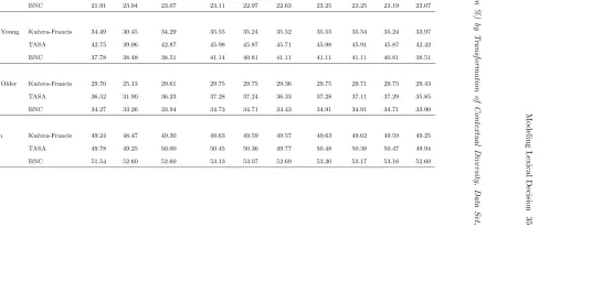
[image:36.595.103.664.121.475.2]M o d el in g L ex ic al D ec is io n 35 4 n ce A cc o u n te d fo r ( R 2 in % ) by T ra n sf o rm a tio n o f C o n te xt u a l D iv er si ty , D a ta S et , o rp u s
Data Corpus rank CD log. CD power CD gen. pow. CD race CD exp. CD APEX CD PEX CD IA1 CD IA2 CD
MF Exp. 1 Kuˇcera-Francis 21.17 20.48 21.73 21.73 21.40 20.57 21.76 21.76 21.65 21.74 TASA 19.94 21.18 21.43 21.92 22.65 22.02 22.67 22.08 22.65 21.40 BNC 21.91 23.04 23.07 23.11 22.97 22.63 23.25 23.25 23.19 23.07
BCP99 Young Kuˇcera-Francis 34.49 30.45 34.29 35.55 35.24 35.52 35.55 35.54 35.24 33.97 TASA 42.75 39.06 42.87 45.98 45.87 45.71 45.98 45.91 45.87 42.42 BNC 37.78 38.48 38.51 41.14 40.81 41.11 41.11 41.11 40.81 38.51
BCP99 Older Kuˇcera-Francis 29.70 25.13 29.61 29.75 29.75 29.36 29.75 29.71 29.75 29.43 TASA 36.52 31.90 36.23 37.28 37.24 36.33 37.28 37.11 37.29 35.85 BNC 34.27 33.26 33.94 34.73 34.71 34.43 34.91 34.91 34.71 33.90
[image:37.595.59.636.165.449.2]M o d el in g L ex ic al D ec is io n 36 ab le 5 a lu es , C o n te xt u a l D iv er si ty . H 0: R a n k Hy po th es is
Data Corpus Ha: log. CD power CD gen. pow. CD race CD exp. CD APEX CD PEX CD IA1 CD IA2 CD
MF Exp. 1 Kuˇcera-Francis .040 .081 .385 .426 .442 .326 .171 .227 .078 TASA .000 .017 .017 .000 .002 .027 .014 .000 .016 BNC .000 .025 .006 .066 .033 .017 .036 .022 .021
BCP99 Young Kuˇcera-Francis .079 .810 .048 .000 .000 .002 .000 .000 .897 TASA .000 .011 .001 .000 .000 .001 .000 .000 .014 BNC .000 .000 .000 .000 .000 .000 .000 .000 .000
BCP99 Older Kuˇcera-Francis .673 .844 .382 .160 .128 .356 .791 .248 .827 TASA .001 .343 .019 .001 .000 .047 .003 .000 .308 BNC .005 .340 .065 .001 .000 .036 .001 .027 .267
Elexicon Kuˇcera-Francis .000 .002 .001 .000 .000 .000 .000 .000 .011 TASA .000 .000 .000 .000 .000 .000 .000 .000 .000 BNC .000 .000 .000 .000 .000 .000 .000 .000 .000
[image:38.595.116.662.158.441.2]M o d el in g L ex ic al D ec is io n 37 6 lu es , C o n te xt u a l D iv er si ty . H a : R a n k h yp o th es is
Data Corpus H0: log. CD power CD gen. pow. CD race CD exp. CD APEX CD PEX CD IA1 CD IA2 CD
MF Exp. 1 Kuˇcera-Francis .003 .533 .302 .103 .008 .345 .434 .325 .481 TASA .064 .197 .502 .839 .229 .443 .292 .857 .143 BNC .277 .383 .524 .171 .072 .566 .396 .519 .376
BCP99 Young Kuˇcera-Francis .000 .002 .426 .979 .178 .842 .467 .967 .000 TASA .000 .000 .173 .853 .001 .228 .268 .827 .000 BNC .000 .000 .574 .985 .336 .428 .441 .991 .000
BCP99 Older Kuˇcera-Francis .000 .009 .266 .446 .000 .247 .073 .414 .002 TASA .000 .000 .393 .082 .000 .231 .033 .428 .000 BNC .000 .000 .133 .021 .000 .129 .225 .012 .000
Elexicon Kuˇcera-Francis .000 .000 .487 .981 .000 .558 .493 .985 .000 TASA .000 .000 .276 .000 .000 .502 .016 .539 .000 BNC 1.000 1.000 .163 .000 .000 .512 .193 .000 1.000
[image:39.595.116.663.158.441.2]M o d el in g L ex ic al D ec is io n 38 ab le 7 a lu es , C o n te xt u a l D iv er si ty . No n -n es te d T es ts E xc lu d in g R a n k
H0: gen. pow. CD PEX CD APEX CD
Data
Corpus Ha: exp. CD APEX CD PEX CD IA1 CD IA2 CD race CD gen. pow. CD APEX CD IA1 CD IA2 CD IA1 CD IA2 CD
MF Exp. 1
Kuˇcera-Francis .333 .549 .743 .561 .618 .522 .458 .193 .547 .665 .642 .730 TASA .038 .441 .273 .498 .117 .129 .998 .994 .999 .948 .715 .141 BNC .758 .597 .651 .958 .619 .472 .497 .603 .551 .589 .720 .697
BCP99 Young
Kuˇcera-Francis .573 .489 .751 .389 .364 .476 .730 .796 .544 .425 .451 .383 TASA .681 .561 .545 .491 .490 .330 .969 .894 .975 .829 .492 .516 BNC .312 .146 .435 .336 .189 .283 .966 .863 .821 .591 .838 .590
BCP99 Older
Kuˇcera-Francis .529 .288 .294 .766 .598 .605 .906 .892 .945 .805 .928 .626 TASA .597 .041 .676 .713 .686 .315 .995 .970 .999 .992 .908 .446 BNC 1.000 .981 .624 .568 .997 .909 .627 .420 .599 .792 .681 .851
Elexicon
Kuˇcera-Francis .565 .978 1.000 .167 .016 .449 .985 .997 .814 .122 .036 .007 TASA .859 1.000 .739 1.000 .245 .080 1.000 1.000 1.000 .984 .078 .045 BNC .999 .999 .985 1.000 1.000 .039 1.000 1.000 1.000 .967 .997 .981
[image:40.595.24.670.99.483.2]Figure Captions
Figure 1. Estimated distribution ofR2 (%) for power law fit to rank hypothesis data, Murray and Forster’s (2004) Experiment 1, using condition means. Number of bootstrap
samples, B= 10,001. Vertical line is observed R2 for power law fit.
Figure 2. Estimated distribution of difference in R2 (%) between power law and rank fits
to rank hypothesis data, Murray and Forster’s (2004) Experiment 1, using condition
means. Number of bootstrap samples, B= 10,001. Vertical line is observed difference.
Figure 3. Estimated distribution of Hotelling T statistic comparing power law and rank fits to rank hypothesis data, Murray and Forster’s (2004) Experiment 1, using condition
means. Number of bootstrap samples, B= 10,001. Vertical line is observed difference.
Figure 4. Estimated distribution of Hotelling T statistic comparing rank and power law fits to power law hypothesis data, Murray and Forster’s (2004) Experiment 1, using
condition means. Number of bootstrap samples,B = 10,001. Vertical line is observed
difference.
Figure 5. Relationship between corpus estimates of frequency. (a) Comparisons involving rank word frequency. (b) Comparisons involving log. word frequency. Whilst the
logarithmic transformation of frequency is approximately linearly related between corpora,
the relationship between ranks estimated from different corpora can be far from linear. As
these ranks were adjusted to accord with undergraduate vocabulary (size), the differences
75
80
85
90
95
100
0.00
0.02
0.04
0.06
0.08
Variance Accounted for (%) by Power Law of Frequency
Density
0
2
4
6
8
10
0.0
0.1
0.2
0.3
0.4
0.5
Difference in Variance Accounted for (%):
Power Law of Frequency − Rank Frequency
Density
Hotelling Statistic:
Power Law of Frequency vs. Rank Frequency
Density
0.0 0.2 0.4
−4 −2 0 2
Hotelling Statistic:
Rank Frequency vs. Power Law of Frequency
Density
0.0 0.2 0.4
−4 −2 0 2
Frequency (per million)
Frequency (per million)
Rank Frequency
Kucera−Francis TASA CELEX
TASA
CELEX
BNC
(b)
(a)
v
0.001
10
100000
0.001
10
100000
0.001 10 100000
0.001 10 100000
0.001
10
100000
0.001 10 100000
(a)
TASA
CELEX
0 10000 20000
0
10000
20000
0 20000 60000
0
5000
15000
0
20000
50000
Kucera−Francis
0 20000 40000
Postscript: Deviations from the Predictions of Serial Search
James S. Adelman and Gordon D. A. Brown
Murray and Forster (2004) claimed that rank frequency provided a better account of
lexical decision times than either log frequency or power law frequency, the latter being
dismissed on the grounds of over-flexibility. We (Adelman & Brown, 2008) argued that (i)
Murray and Forster’s use of the relatively small Kuˇcera and Francis (1967) word frequency
counts biased the estimates of rank; (ii) the superiority in fit of the power law (and of some
other functions) could not all be attributed to over-flexibility in the manner Murray and
Forster claimed; and (iii) bootstrapping analyses designed to take flexibility into account
gave evidence of systematic deviations from several theoretically-motivated functional
forms, including rank and power, but not from some generalizations of the power function.
We concluded that the data could not be taken as support for serial search models.
Murray and Forster (2008) have suggested that our results do not contradict the
rank hypothesis (and in fact support it) because (i) an additional task-specific mechanism
could account for any discrepancy between data and model predictions; (ii) the increase in
R2 for rank when better-estimated ranks are used provides stronger evidence for rank, and
shows that the case for rank was not favored by a bias in rank estimates; (iii) Adelman
and Brown (2008) did not find a systematic failure of the rank function; (iv) assessment of
the rank function does not rely on estimation of parameters, but assessment of the power
function relies on parameters that lack theoretical interpretation or independent
justification, unlike those of the rank function; (v) their simulations of an instance model
show that such models cannot provide a plausible account of mean lexical decision
latencies; and (vi) data from different tasks, data sets, and measures converge in favor of
the rank function.
In response to Murray and Forster’s (2008) comments, we make the following
points. (i) An appeal to additional mechanisms can of course be made for any theory, but
— absent a detailed specification and test of such mechanisms — such appeal inevitably