Development of a vane motor servo system for precision positioning in an MRI or CT environment

Acknowledgements

Doing research and writing this thesis has been a long and interesting experience, at times fun, at times tough. I wouldn’t have been able to reach this point without the many people around to support me.

First of all, I want to thank my parents, Anja and Mieke, for being extremely supportive of me all throughout my education these past 20 years. Without their unending support I would definitely not be here.

All of my friends deserve a thanks as well. During a time where all day, every day, is dominated by this thesis, they have been indispensable in showing me that there is, in fact, life besides graduating. The great times we had definitely helped reduce stress.

I would also like to thank my daily supervisor at Demcon, Maarten Arnolli. When he was not busy crossing 250 km of ice days before receiving his PhD, he would always be there to give constructive, useful, and sober advice for the project during our weekly meetings. I feel that our sparring has really improved my understanding of mechanical and control concepts.

Thanks also goes to my supervisors from the University of Twente, Vincent Groenhuis and Franc¸oise Siepel. They were always just a small bike ride away and ready to give valuable input for my research and report.

Summary

Electromechanical actuators are widely used in a range of applications because of their good speed, torque, and bandwidth characteristics. In a CT/MRI-environment, their application is limited as the materials used can cause da-mage to the system and patient, or degrade ida-mage quality. There is a need for precise actuators that can function in a CT/MR-environment without the aforementioned complications.

Various systems have been developed for use in a CT- or MRI-scanner [1, 2, 3]. However, these systems generally suffer from not being completely MRI-compatible or from having poor precision or speed characteristics.

The main objective of this thesis is to explore the possibilities of, and to develop, an actuator system that can be used to precisely position a needle guide in a CT- and MRI-environment.

Due to its high power-to-weight ratio, inherent cleanliness, simple design, and promising positioning precision [4, 5], a pneumatic vane motor forms the basis of a novel actuator system designed in this thesis.

Other works of literature cover the subjects of CT/MR-compatible actuation [1, 2, 3, 6] and positioning of vane motors [4, 5] separately. This thesis uses the knowledge on CT/MR-compatible actuation to design a pneumatic system that can be used in a CT- or MRI-scanner. An important distinction with normal positioning of vane motors in e.g. [4, 5] is that control valves, which typically use solenoid actuation, can not be present near the vane motor. Valves and actuator are separated by 5 meters of tube, introducing a delay into the system.

Dynamical behaviour of the vane motor is described using models from literature. The filling and emptying of pneumatic tubes is modelled as well. Insight gained by this modelling serves as the basis for a novel system design which includes valve and tube topology. A non-linear simulation model and a proof-of-principle setup are created from this system design.

Identification using the lab set-up and the non-linear model is done to clarify various system characteristics, such as the relation between torque and angle, which is non-linear. Several Linear Time-Invariant (LTI) input/output models are fitted to experimental data.

Three controllers are designed to achieve precise positioning results: a PID controller, a state feedback controller, and a controller utilising a brake attached to the vane motor’s shaft.

PID control is implemented on the lab set-up to analyse the vane motor servo system’s performance for various scenarios. In the majority of scenarios where control valves are placed close to the vane motor, a precision of 0.5ois achieved in 100% of the cases; other experiments attained a precision of 1o, in line with design goals. When tubes of 5 meters are placed between actuator and control valves, to simulate control valves being placed outside of the MRI bore or CT zone, 1oprecision is achieved within 10 seconds in 90% of the cases.

Contents

1 Introduction 5

1.1 Research context . . . 6

1.2 Objective . . . 7

1.3 Outline . . . 7

2 Background 8 2.1 Objective . . . 8

2.2 State of the art . . . 8

2.2.1 Computed Tomography . . . 8

2.2.2 Magnetic Resonance Imaging . . . 9

2.2.3 CT- and MR-compatible actuation principles . . . 10

2.2.4 Choice of actuator . . . 14

3 System design and modelling 17 3.1 Objective . . . 17

3.1.1 Requirements . . . 17

3.2 Materials & methods . . . 19

3.2.1 Vane motor operating principle . . . 19

3.2.2 Dynamic model . . . 20

3.2.3 Tubes and valves model . . . 25

3.2.4 System design . . . 26

3.3 Results . . . 28

3.3.1 System design . . . 28

3.4 Discussion . . . 31

4 System identification 32 4.1 Objective . . . 32

4.2 Materials & methods . . . 32

4.2.1 Torque-angle relation . . . 32

4.2.2 Motor speed and torque . . . 32

4.2.3 Pressure dynamics . . . 33

4.2.4 Dynamic response . . . 33

4.3 Results . . . 37

4.3.1 Torque-angle relation . . . 37

4.3.2 Motor speed and torque . . . 39

4.3.3 Pressure in tubes . . . 39

4.3.4 Dynamic response . . . 41

5 Controller design 47

5.1 Objective . . . 47

5.2 Materials & methods . . . 47

5.2.1 PID control . . . 47

5.2.2 State feedback controller . . . 50

5.2.3 Brake control . . . 53

5.3 Results . . . 53

5.4 Discussion . . . 54

6 Performance analysis 56 6.1 Objective . . . 56

6.2 Materials & methods . . . 56

6.2.1 Experiments . . . 56

6.3 Results . . . 57

6.4 Discussion . . . 58

7 Conclusions & outlook 61 7.1 Conclusions . . . 61

7.2 Discussion . . . 62

7.3 Outlook . . . 64

References 66

Chapter 1

Introduction

Over the past decade, the number of yearly Computed Tomography (CT) and Magnetic Resonance Imaging (MRI) scans in the Netherlands has tripled [7, 8]. Simultaneously, technological advances allowed surgery to transition from open procedures, where incisions are made in the patient’s body to access various sites, to minimally invasive procedures. Laparoscopy, angioscopy, and endoscopy are some minimally invasive surgical procedures. Percutaneous surgery, where access to a patient’s internal sites is provided via a needle-puncture of the skin, is minimally invasive as well. Examples of percutaneous procedures include biopsy and tissue ablation using radio-frequency (RF) or microwave (MW) radiation.

Working in an MRI- or CT-environment imposes constraints on the materials which can be used, and therefore on the type of actuation. It is desirable to make a system that is fully CT- and MR-compatible. Different terminologies exist for CT- and MRI-compatibility. CT-compatibility is defined as the system being sufficiently X-ray transparent to avoid unacceptable image distortion. For MRI, the terminologies adopted by the US FDA are as follows. A system or object is MR-safe if it poses no known hazards to the patient or environment in the form of magnetic or induced forces, torques, RF heating, or induction of voltages. The rationale behind MR-safeness of a material should be grounded in scientific reasoning instead of tests [9]. If a system is safe to use in MRI-scanners up to a certain field strength, the system is dubbed MR-conditional.

MR-safeness considers only hazards in any form to patient, radiologist, or environment. MRI-compatibility of a system considers the effect of an MR-safe device on the diagnostic image data as well. Akin to CT-compatibility, MRI-compatible systems avoid unacceptable image distortion.

Various robotic systems have been developed to improve minimally invasive surgical procedures with varying degrees of automation [1, 3]. Some of these systems use piezoelectric actuation, which makes them inherently not MRI-compatible. Pneumatic actuators in a CT or MRI context are often in the form of stepper motors. Some of these systems, such as the PneuStep [10], are complex in design. Other pneumatic stepper motors generally suffer either from low bandwidth or low resolution.

CT/MRI-compatible robotics. This development includes: a choice of actuator type, design of a system that interfaces the actuator with its environment, and a mechanical design of the actuator with a focus on CT/MRI-compatibility.

This research focuses on picking a suitable actuator, identifying its under-lying mechanics and challenges, and designing a controller with which to accurately position the actuator.

1.1

Research context

A novel system for use in a CT-scanner is the Needle Placement System (NPS) developed by DEMCON, see Figure 1.1. The NPS provides physical guidance of a needle for manual insertion in the liver and lungs. When a patient develops a liver tumour, the usual procedure is to remove it surgically. This is often done by ablating the tumour’s cancerous tissue with microwave radiation. Ablation is a complex process and as such, surrounding healthy tissue is often removed as collateral damage. To minimise the damage to a patient’s healthy tissue, it is imperative that the needle be placed accurately. In the traditional work flow, the physician places the patient inside a CT- or MRI-scanner to assess the tumour’s location, orientation, and size. With the help of several markers which show the angle with respect to the patient’s body, the physician aims and inserts the needle manually. As tumours can be quite small at around 2 cm, and situated deep inside the patient, the physician often does not place the needle correctly in one try. This leads to patient inconvenience and higher costs.

Figure 1.1:Impression of the DEMCON NPS.

The NPS, pictured in Figure 1.1, automates part of this process. It receives and interprets CT-scans automatically, plans a path for the needle to the tumour, and aligns two segments (seen in the left of the picture) with a precision of 0.01o. Positioning is achieved by two DC motors and a 1:100 transmission. The physician then places a needle inside the needle guide and manually inserts it to the correct depth.

Currently, the NPS uses electromechanical actuation at the base of the arm, which is transmitted via cables to the end-effector. Since the motors them-selves are outside of the scanning zone, they produce no problems with the CT-scanning process. In an MRI-scanner, DC motors pose risks for patient and environment. The NPS is thus not MR-safe. If the NPS is to be made MRI-compatible as well, an alternative method of actuation will have to be developed that is inherently CT- and MRI-compatible.

1.2

Objective

The main objective of this research is:

To develop a servo system for precision positioning of a needle guide in a CT-or MR-environment

This objective comprises making a design of the hardware on a system level, creating a model of the system, realisation of the system in a proof-of-principle set-up, system identification, controller design, and performance assessment. A

redesign of the actuator to a version made out of MR/CT-compatible materials is not made in this thesis. The first step when developing a new actuator for the NPS is to evaluate its performance. Changing the design of an actuator slightly to accommodate CT/MRI-compatible materials is not seen as an important goal of this research. A few notes on the actuator’s redesign are given in Chapter 7.

1.3

Outline

Chapter 2

Background

2.1

Objective

The objective of this chapter is to provide a background in CT- and MR-compatible actuation, and to choose an actuator for the rest of this thesis.

2.2

State of the art

In order to make an informed decision about the type of actuator to use in this thesis, it is necessary to explain more about image modalities such as CT and MRI. These processes are discussed in this section, as are materials which can be used in both methods.

2.2.1

Computed Tomography

Computed tomography (CT) provides 2D and 3D cross-sectional images recon-structed from multiple projectional images. A picture demonstrating this can be found in Figure 2.1. On one side of the patient, an X-ray source is located, which emits X-rays through the patient and into the X-ray sensors on the other side. The amount of absorption then provides information about the material in between. By spiralling the source and sensors around the patient, a full 3D image can be reconstructed. Contrast material can be injected into the patient to highlight e.g. the blood vessels.

X-ray transparency of materials Since the scan output depends on the materi-als that the X-rays pass through, care should be taken about which materimateri-als are present in the CT-scanner. Materials which absorb or scatter radiation should be avoided. X-ray intensity Itafter passing through a material of thicknesst, with initial X-ray intensityI0is defined according to Beer’s law:

It(t) =I0e−µ(E)t, (2.1)

whereµ(E), is the material-specific X-ray absorption coefficient, dependent on energyE. Beringer [11, Figure 31.16] shows that the absorption length of radio waves becomes smaller as the atomic number of the material becomes

higher. This means that materials with high atomic numbers, such as iron and copper, are undesirable in CT-scanners. Since plastics and ceramics are mostly comprised of smaller atoms such as carbon, silicon, hydrogen, and oxygen, these materials will not distort the quality of a CT-scan as much.

Figure 2.1:Process of a computed tomography scan [12].

2.2.2

Magnetic Resonance Imaging

Magnetic Resonance Imaging (MRI) relies onnuclear magnetic resonance(NMR) to create an image of a patient. NMR is the process where atomic nuclei absorb and re-emit electromagnetic radiation when exposed to a magnetic field. The resonance frequency at which this happens depends on the magnetic field properties and on the properties of the isotope that is being excited. Specifically, isotopes with an odd number of protons and neutrons have an intrinsic magnetic moment (spin), and produce NMR spectra. When an isotope with a magnetic moment, such as hydrogen or carbon, is placed in a magnetic field, its magnetic moment aligns with the field direction.

A change in field strength then causes the protons to change their alignment. When changing back to their original orientation, a magnetic flux is produced, which changes the voltage in receiving coils that process the signal.

Since the resonance frequencies vary linearly with field strength, a spatial gradient can be applied to the magnetic field strength. Based on the detected resonance frequencies, a 3D-image can be obtained showing the location and amount of e.g. water in a patient’s body. This can then be used to deduce the composition of tissue in various locations.

MR-safe, -conditional, and -compatible materials Because a magnetic field is present in the MR bore, materials that are magnetic will experience a force and/or torque. Depending on the nature of this magnetic field, conductors can be displaced, risking damage to both the patient and machine. If a DC magnetic field is applied, conductors which are moving experience forces, torques and currents. If the magnetic field is AC, conductors which are at rest are affected as well.

2.2.3

CT- and MR-compatible actuation principles

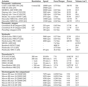
In this section, several methods of actuation that are used in a CT or MR environment are discussed. For each method, advantages and disadvantages will be given, along with approximate values for resolution, speed and power. All statements made are backed up with references either to actuators that are on the market at the time of this writing, or to a paper that shows these performances. A summary of each actuation type’s strengths and potential design challenges can be found in Table 2.2. An overview of several actuators for each type, along with their performance, is found in Table 2.1.

Pneumatic actuation

Air motors have a high power-to-weight ratio, are simple in design, are self-cooling, and can be used in volatile environments where sparking could result in an explosion [4]. Air leakage poses low risks in most environments, and exhaust air can be returned to the atmosphere. Furthermore, its design allows for an MRI-compatible version by adequate material selection. Pneumatic motors have been deployed in e.g. functional MRI (fMRI) actuation [13, 14]. Pneumatic actuators can be divided in continuous and stepper motors.

Continuous motors The first type of pneumatic actuators operate as long as power is supplied. Once power supply is stopped, the motor stops moving. Theoretically, a continuous motor is able to be positioned in any configuration. Several continuous pneumatic actuators exist, such as the vane motor (see Figure 2.2), the harmonic drive, and the piston.

(a) Working principle of a vane motor, which exist in both pneumatic and hydrau-lic versions [15].

(b) A pneumatic vane motor as developed by NSK.

Figure 2.2: Pneumatic motors, operation principle (left) and example motor (right).

Continuous pneumatic actuators are being used in MRI [16], though litera-ture on the subject is scarce.

Pneumatic actuation, in the form of both continuous and stepper motors, suffers from the compressibility of air. In [17], a linear force controller was

made for a pneumatic actuator with low friction. The authors achieved a 16 Hz bandwidth for±2 N force changes. By using a complex non-linear model and sliding mode controller, Richer et al. increased the bandwidth to 58 Hz [18]. There is also a lot of friction present in pneumatic systems, which make them hard to control. Still, accurate positioning of a ball screw table actuated by a pneumatic vane motor was achieved in [4]. The authors report a positioning error of 6 mrad by using sliding mode control.

Stepper motors The other type of actuator is powered by alternately filling and evacuating a chamber with air, which causes a mechanism to engage and disengage accordingly. Stepper motors are capable of moving only in certain increments defined by the system’s geometry. This poses a hard limit on the achievable precision. Figure 2.3 depicts a linear pneumatic stepper motor.

Figure 2.3:Example of an MRI-compatible pneumatic stepper motor [19].

Bandwidth is also a major challenge for stepper air motors. In [20], a band-width of 10 Hz was achieved for tubes of 5 meters.

Compared to continuous actuators, MRI-compatible pneumatic stepper motors are more numerous in literature. The PneuStep, developed in [10], has a resolution of 3.3oand a maximum speed of 180 rotations per minute. A more recent example are the T-63, R-80, and differently sized counterparts developed in [20]. These stepper motors are completely metal-free. The rotary motors have a resolution of 10o_{and a speed of 133 rpm, while the linear motors have a} resolution of 1 mm and a speed of 200 mm/s.

Hydraulic actuation

which should be assessed as a potential cause of a hazardous situation in risk management.

Hydraulic actuation was compared with pneumatic actuation in a MR-environment by Yu et al. [22]. A device was developed with one translational DOF to be used by a patient in fMRI tasks. The actuator was a piston cylinder, either hydraulic or pneumatic. The authors reported that the hydraulically actuated system achieved a higher positioning accuracy, smoother movements and a greater robustness against force disturbances than the pneumatic system. On the other hand, the pneumatically actuated piston is backdrivable and had better force control.

Electrical actuation

Two types of electrical actuators are discussed: piezoelectric motors and electro-active polymer (EAP) actuation. Their reliance on electrical and magnetic fields make them MR-conditional at best.

Piezoelectric actuation The electric dipole moment of atoms in a crystal struc-ture varies between regions, the so-called Weiss domains. In some solids, applying a mechanical stress aligns the dipoles of these domains. This creates a change in polarization, which produces a current. This is called thepiezoelectric effect. It is seen to occur in some synthetic ceramics and plastics, but also in natural materials such as wood and DNA.

In piezoelectric materials, the converse effect also occurs, where a deforma-tion is created by applying an electrical field to the crystal. This is the basis of piezoelectric actuation. An example of a piezoelectric actuator is shown in Figure 2.4. The piezomotor slowly extends, then rapidly contracts, producing a force which moves the base. By accurately controlling the electrical field, very high resolutions can be achieved, even under 100 nm [23]. The large bandwidth of electrical systems is also an advantage here, meaning high speeds can be achieved. These properties make piezoelectric actuation popular among MR-conditional systems: in [24], a 9-DOF robot was designed for minimally invasive interventions in the prostate, which makes use of several ultrasonic motors to position, insert, and steer a needle. A compliant force-feedback ultrasonic actu-ator for wrist protocols during functional MRI was designed, built and tested in a 3 T MRI scanner [25].

Piezoelectric actuators experience a lot of friction by design, quickly leading to wear. The actuators are also non-backdrivable, so a more complex design is needed to make a system that is backdrivable. Although they are not magnetic, piezoelectric actuators produce artefacts in MRI scans, especially when turned on [27, 28]. When the actuators are covered in RF-shielding material such as aluminium, some authors report an improvement in the signal-to-noise ratio (SNR) [29]. Still, most studies are done in 1.5 - 4.0 T scanners, while magnets with field strengths up to 11 T are already developed for use in high field neuroimaging [30], making the MR-compatibility of piezomotors questionable.

Electroactive polymer actuation Electroactive polymers (EAPs) resemble pie-zoelectric materials in that they also deform when an electric field is applied.

EAPs however exhibit much larger strains of up to 200% and are popularly referred to as artificial muscles.

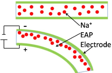
EAPs come in two types: dielectric and ionic EAPs. The first type relies on electrostatic forces which shrink the polymer in thickness and expand it in area. These EAPs have a fast response time and can provide large actuation forces. A strain can be maintained by a DC voltage. The electric field needed to deform a dielectric EAP (DEAP) is high, however, with values of 100 MV/m cited [31]. Ionic EAPs (IEAPs) provide actuation by displacing ions inside a polymer (Figure 2.5). They require an electrolyte to provide actuation. Their main advantage is that they require a relatively low operating voltage (1-3 V) and are generally bi-directional. However, the electrolyte can evaporate over time, making the material dry and decreasing performance. IEAP response times are much higher than DEAPs (100 ms vs 1 ms). For most IEAPs, it is difficult to maintain a displacement by applying a DC voltage [31].

The MR-compatibility of a DEAP was tested in [32]. It was found that an applied electrical field of 8 MV/m on the DEAP produced almost no difference in SNR in a 3 T MRI scanner. In [33], the authors produced a linear DEAP actuator which is capable of lifting a 7.5 kg mass 2.2 mm, and deflecting a spring by 2.2 mm, producing a force of 66 N. A commercial EAP-based motor has yet to be developed.

Remote actuation

It is possible to use electromagnetic actuation, as long as the actuators them-selves are either not in the way of X-ray beams (in CT) or are outside the MRI bore. This means that transmissions, such as a cable/belt or rod, are needed to control the end-effector.

Electromagnetic DC motors are the actuation method of choice for most robotics applications. They have a high bandwidth, are usually backdrivable and allow for simple control of position and force. The working principle of a DC motor is shown in Figure 2.6. By alternating the current’s direction inside a coil, the armature is alternately attracted and repelled by two permanent static

(a) Working principle of a pie-zomotor [26].

(b) Example of a piezoelectric motor as developed by Piezo-motor.

Figure 2.5:Working principle of an ionic EAP motor [34].

magnets around the armature. In a MR-environment, these motors have to be placed at a safe distance from the magnet’s isocenter. Even then, shielding may be required. In [2], a DC motor was placed at a distance of 2.5m from the isocenter of a 1.5 T MR scanner. The motor was then repeatedly switched on and off, keeping track of an object’s SNR in the scanner bore. This was done with and without shielding by a mu-metal. When the motor was not shielded, SNR changed heavily depending on if the motor was running or not. After applying shielding, SNR remained relatively constant throughout the experiment. Keeping in mind the increase in scanner strength, the actuators would have to be placed further away from the bore, making it difficult to design a compact and efficient electromagnetically actuated MR-safe robot.

(a) Working principle of a DC motor [35].

(b) Example of a DC motor as developed by Maxon.

Figure 2.6:DC motors, operation principle (left) and example motor (right).

2.2.4

Choice of actuator

Various actuation principles have been considered in search of a CT and/or MRI-compatible motor, and a wealth of designs has been developed. However,

Table 2.1:Overview of a selection of actuators, with specifications. Actuator specifications were found in ranges corresponding to the application in this thesis.

Actuator Resolution Speed Force/Torque Power Volume (cm3₎

Pneumatic: continuous

GAST 1AM-NRV-39A [36] 6 mrad [4] 10000 rpm 0.75 Nm 300 W 326

NSK EX-203c [37] - 25000 rpm - - 18.8

MORITA AIR TORX [38] - 20000 rpm 0.03 Nm 10 W 22.5

Deprag Adv. Line 67-010 [39] - 3000 rpm 0.06 Nm 20 W 48

Deprag Adv. Line 67-030 [39] - 1300 rpm 0.29 Nm 20 W 50.6

Modec Air motor MT051_{1 [40] - 2772 rpm 2 Nm 92 W 253.7}

Desoutter MR16 KL-ATEX [41] - 13000 rpm 0.15 Nm 110 W 75

Desoutter MR25 KL-ATEX [41] - 13100 rpm 0.24 Nm 160 W 137.4

Pneumatic: stepper

Groenhuis R-44 (stepper) [20] 10◦ _{333 rpm 0.45 Nm 3.7 W 60}

Groenhuis R-25 (stepper) [20] 6.9◦ _{231 rpm 0.1 Nm 1.1 W 12.5}

PneuStep (stepper) [10] 3.3◦ _{180 rpm 0.6 Nm 3 W 198.6}

Hydraulic

HydroLeduc PB32.5 [42] - 5000 rpm 0.27 Nm 22 W 122.4

HydroLeduc PB36.52_{2 [42] - 5000 rpm 0.69 Nm 57 W 268.6}

HydroLeduc PB1.3 [42] - 4000 rpm 7.6 Nm 600 W 726.4

MOOG A085 [43] - - 7.4 Nm - 6135.8

Bansbach HZ163_{3 [44] - - 4000 N - 28.4}

Flodraulic LP-12 [45] - - 4.75 Nm - 219

Flodraulic MPJ-11 [45] - 69 rpm 36.4 Nm 42 W 210.7

Piezoelectric4₄

PI N-412.50 [46] 300 nm 20 kHz 7 N 0.042 W 10.2

PI M-664.164 [47] 200 nm 400 mm/s 4 N 1.6 W 81

DSM I-90 [48] <1µm 30 mm/s 90 N 2.7 W 64.6

DSM I-30 [48] <1µm 30 mm/s 30 N 0.9 W 16.1

NanoMotion HR1 [23] <100 nm 250 mm/s 3.5 N 0.875 W 8.3

NanoMotion HR2 [23] <100 nm 250 mm/s 7 N 1.75 W 13.5

Electromagnetic (for comparison)

Maxon RE-max 24 222049 [49] - 7470 rpm 0.0525 Nm 9 W 14.5

Maxon RE-max 24 222053 [49] - 9270 rpm 0.0519 Nm 9 W 14.5

Maxon RE-max 29 226802 [49] - 9350 rpm 0.299 Nm 9 W 29.7

Maxon RE-max 29 226806 [49] - 8860 rpm 0.299 Nm 9 W 29.7

Maxon DCX 22 12V [50] - 6240 rpm 0.015 Nm 8 W 12.9

Maxon DCX 22 24V [50] - 6384 rpm 0.014 Nm 8 W 12.9

a compact and high performance solution that lives up to the way electrical servomotors dominate the field of regular mechatronics is yet to be found.

Pneumatic continuous actuation is often dismissed due to non-linear beha-viour and a high amount of friction [6]. Precise positioning using a pneumatic vane motor has however been shown feasible [5, 4]. The vane motor furthermore offers a high power-to-weight ratio, cleanliness and simple design of which an MR-compatible version has readily been developed [16]. This makes the vane motor an excellent candidate for a CT- and/or MRI-compatible actuation system.

1 _{Not reversible.} 2 _{Non-backdrivable.} 3 _{Maximum load time 10 s, 15% of duty cycle.} 4 _Powers

Table 2.2:Summary of several actuation types used in an MRI-environment, with their advantages and challenges listed.

Actuation type Advantages Challenges

Pneumatic ◦High

power-to-weight ratio

◦Low bandwidth

◦Safe in volatile envi-ronments

◦Losses due to leakage

◦Leakage not a safety issue

◦Low efficiency

◦Completely MR-compatible

◦Large amounts of friction

Continuous High speeds attainable ◦Position control

difficult

Stepper ◦Position control

sim-ple

◦Resolution and speed limited by geometry ◦Higher friction than continuous motors

Hydraulic ◦High

power-to-weight ratio

◦Leakage can be an issue

◦High stiffness ◦High inertia due to fluid

◦Actuation principle is MR-safe

◦High friction

◦High pressure allows for high torques

Piezoelectric ◦Extremely high

reso-lution

◦Not completely MR-safe

◦High bandwidth ◦Not backdrivable ◦High amount of wear ◦Low power

◦Not X-ray transparent

Electroactive polymer: DEAP

◦High forces possible ◦Need a strong electric field

◦High energy density ◦Actuation mostly uni-directional

◦Fast response time ( 10−3_s)

◦Not available as mo-tor yet

IEAP ◦IEAP: Bi-directional ◦IEAP: Performance degrades material dries ◦IEAP: Low voltage

required

◦IEAP: Slow response time ( 10−1s)

◦Not available as mo-tor yet

◦IEAP: Requires electrolyte

Remote actuation ◦Standard servomotor

possible

◦Reducing friction

◦Achieving sufficient stiffness

Chapter 3

System design and modelling

3.1

Objective

The objective of this chapter is to develop a vane motor servo system with control valves and tubes in favour of precision position control. A non-linear model is constructed of the system, which is then built in the form of an experi-mental set-up to test several strategies for positioning. These strategies include adjustable friction torque and tube lengths. First, a list of requirements is made.

3.1.1

Requirements

Requirements can be divided into a few categories: what the systemmust

achieve, what the systemshouldachieve, and what itcouldachieve.

There is only one requirement thatmust be achieved, which is that the system is CT- and MRI-compatible. This means that no magnetic or conducting materials can be used. Materials with a high atomic number have to be avoided as well, as they absorb X-rays. The other requirements,shoulds andcoulds, are named design goals.

Design goals are not as strict. For instance, the torque specification is not set in stone, as several alterations to the NPS can be made to accommodate a lower torque output by the vane motor. In practice, this means that an off-the-shelf actuator will be picked to do experiments on. Within this constraint, the maximum achievable performance for torque, rotational velocity, and precision will be evaluated for several scenarios. The design goals are listed below.

Precision The motor should achieve a precision of 1o. This is based on the minimum tumour size that has to be punctured, which is 5 mm in diameter. The NPS’ end-effector precision is 0.01o. The end-effector is linked by a worm to the actuators with a 1:100 transmission. The actuators themselves thus achieve a precision of 1o. The chosen actuator should be able to achieve this precision as well.

This torque originates from several sources. To aid the explanation below, an impression of part of the NPS is shown in Figure 3.1. A simplified iconic diagram of the vane motor and NPS is shown in Figure 3.2.

Figure 3.1: Impression of the NPS’ segments and drive axis, including worm wheels (green) and pre-load torsion spring (white).

The vane motor is connected to a worm, which forms a 100:1 transmission with a worm wheel. This worm wheel is connected to a shaft which in turn rotates the NPS’ segments. These segments produce a friction torqueTf on the worm wheel axis.

A pre-tensioned torsion spring (Figure 3.1) serves to keep the worm wheels aligned with the actuators’ worms. The maximum torque, Ts in Figure 3.2, produced by this spring is 300 Nmm.

Finally, there is a load torque which is determined by the amount of moving mass. This torque is also after the transmission, so the equivalent inertia is 1/10000th_{of the original inertia.}

Figure 3.2:Simplified iconic diagram of vane motor and NPS. The vane motor has inertia Jm and generalised coordinateφindicating its rotation. A worm is attached to the vane motor which forms a 100:1 transmission with a worm wheel, which is connected to the rest of the NPS, which has an inertia ofJNPS. Gear transmissions in the NPS lead to a friction torqueTf. A pre-loaded torsion spring designed to keep the worm wheel in place produces torqueTs.

The total torque was determined by actuating the worm wheel with a Maxon RE-max 24 222053+201940 motor, which has a motor constant of 24.4 Nmm/A. Movement started at a current of 0.3 A, which means the static torque equals 7.32 Nmm. Dynamic torque was found by determining the steady-state current

when the worm wheel is rotating, found to be 0.22 A. This leads to a dynamic torque of 5.5 Nmm.

Rotational velocity The motor should achieve a speed of 40 RPM. This is based on the worst-case scenario where the NPS has to perform a homing procedure of its entire range of motion (340 degrees per DOF), after which it gets a set-point of 340 degrees again. The desired positioning time is 5 seconds, which means that a rotational velocity of 2.5 rad/s is needed at the end-effector. The current design incorporates a transmission of 1:100 between end-effector and actuator, yielding a rotational velocity of 250 rad/s or 14,000 deg/s of the actuator.

3.2

Materials & methods

This section covers the vane motor’s operating principle and introduces several models from literature. Using these, a novel system design is made based on arguments from a physics and control standpoint.

3.2.1

Vane motor operating principle

A vane motor’s operation is not unlike that of a waterwheel. In this case, pressu-rized air enters a chamber that consists of two eccentrically placed cylinders, the stator and rotor. See also Figure 3.3. The chamber is divided into compartments by vanes, which are pushed against the stator by either centrifugal force, pres-surized air, or springs at the base. Air enters one compartment and as the rotor rotates, the chamber is sealed and expands until it reaches the outlet (here at the bottom). Here, air is exhausted to a lower, typically atmospheric, pressure. The air which is still in the compartment is then slightly compressed as it completes its rotation.

The pressure difference produces a force on the vane between the two adjacent compartments, which constantly varies throughout one rotation. The sum of all the vane forces then produces a torque on the rotor, causing the vane motor to accelerate. Vane motors have a simple operating principle, are compact, and thrive at high rotational velocities. For this reason, they are often used in speed control applications, such as a dentist’s drill. In this thesis however, the positioning accuracy of the vane motor is important.

As stated in Section 2.2.3, there are several challenges in accurate positioning of a vane motor. The first is that there is a large amount of friction present in the system, especially at the vanes’ contact point with the rotor. This introduces some stick/slip-behaviour to the system which makes positioning at low speeds harder to accomplish.

Next, since there are several distinct positions in which the combined torque on the rotor is lowest, there is a possibility that the system will exhibit cogging behaviour at these positions. One such position is when a compartment has just exhausted its air to the outlet, as the work done by that chamber suddenly drops to zero.

Figure 3.3:Working principle of a vane motor[15].

the gas behaves as an ideal gas, is between 0.97 and 0.99. The compressible flow can be interpreted as a stiffness between actuator and end-effector. The system should then be designed such that the influence of the effects mentioned above is as small as possible.

3.2.2

Dynamic model

This section will discuss the dynamic model of the vane motor system, which includes, aside from the vane motor itself, the tubing to and from the actuator, and the control valves. It will take several models from literature on the geo-metry and kinetics of the vane motor, and combine them with a model for the filling and evacuating of pressurized air tubes. The model is then implemented in Simulink to gain insight about the vane motor system’s inner workings and to aid in the future design of a vane motor.

Vane motor dynamics

The vane motor model should capture the change in pressure during rotation of the rotor, the torque produced by a pressure difference between compartments, and the resulting acceleration, rotational velocity, and angle of the rotor as a result of this torque. The first step in describing the relation between pressure and torque is analysing the vane motor’s geometry. Part of this model is taken from [4], where a rotational accuracy of around 1 degree was achieved. The part about work per cycle and mass flow is partly taken from [51], which is a general introduction to vane motors. No performance is mentioned in that paper.

Geometry Consider a motor with Nv vanes, which has a length of L. The angle between vanes isγ= 2_Nvπ. LetRbe the stator’s radius andrthe rotor’s radius. The eccentricitydis defined asR−r. The stator and rotor angles,αand βrespectively, are shown in Figure 3.4a.

Their relation is defined as [51]:

β=α−arcsin

dsin(α)

R

(3.1)

The effective surface area of the vanes is a function of angle. It depends on the working radiusxp, which is defined as [4] (see Figure 3.4b)

xp=

q

d2_sin2_{β+ (R−dcosβ)}2 _(3.2)

(a) Rotor (α) and stator (β) angles of a vane

motor [51].

(b) Working radiusxpfollows from Pytha-goras’ theorem.

Figure 3.4:Vane angles and working radius.

The volumeVαcan be found by a subtraction of integrals and is equal to:

Vα=

L

2(R

2

β−r2α−dRsin(β)) (3.3)

There are three different scenarios for the working volumeVw, i.e. the volume in one compartment:

Vw=



 

 

Vα 0<α≤γ

Vα−Vα−iγ γ<α≤2π

V2π−Vα−γ 2π<α≤2π+γ

(3.4)

Here,Vα−iγ, i=1, 2, ...,Nvequates to the volume oficompletely filled

cham-bers, andV2πequals the volume of all vanes.

Figure 3.5 shows an example. Suppose one is interested in computing the volume of compartmentI I I, shaded with diagonal stripes. Sinceα>γ, working volumeVwequals:

Vw =Vα−Vα−iγ=VI+I I+I I I−VI+I I (3.5)

The These equations can then be used to compute the dead, filled and expanded volumes, see Figure 3.6. The ratio of expanded to filled volume determines the expansion ratio,

e= Vexp

Figure 3.5:Example of chamber volumes for a vane motor with 5 vanes.

which can be interpreted as the extent to which internal energy of the incoming air is used. Ife=1.0, then the pressure remains constant from intake until the exhaust is reached. This means that there is no extra work done by pressure differences between compartments. A high expansion ratio, on the other hand, means that much of the internal energy is used to power the engine. While this leads to higher torques, the water in the supplied air can freeze, causing potential harm to the engine [51].

Figure 3.6:Dead, filled and expanded volumes of a compartment [51].

Work per cycle In order to compute the amount of work done per revolution, a PV diagram is constructed. It is shown in Figure 3.7.

Air enters the motor ata, with pressurePu. As the compartment rotates, it is filled until its volume reachesVf ill, still atPu. Frombtoc, the air expands to

VexpandPue, which can be calculated by assuming a polytropic process:

Pue=Pu

Vexp

Vf ill

!n

=Puen (3.7)

wherenis the polytropic index, typically taken to be 1.3 for air.

Figure 3.7:Pressure-volume diagram of the vane motor [51].

Now the air is exhausted to the surroundings, dropping its pressure toPu. Fromdtoe, the reverse process ofb→coccurs; air, now at ambient pressure, is slightly compressed toPe2:

Pe2=Pee−n (3.8)

This compression produces negative work. Ate, most of the air is released to the other port, leaving only the dead volumeVdin the compartment at state

f.

The total work done by one compartment during one stroke of the engine is given by

W =Wexpansion+Wdisplacement+Wcompression

=− Z b

c pdV− Z

pdV− Z d

e pdV = PuVf ill

n−1 (e

1−n_{−1) + (P}

u−Pd)(Vf ill−Vd) +

PdVexp

n−1 (e

n−1₋₁₎

(3.9)

Mass flow to and from vane motor In a real setup, air entering the chamber does not necessarily have the same pressure as that leaving the compressor. This is due to pressure losses over long and narrow ducts. To simulate this, lumped volumes are placed at inlet and outlets. The mass and pressure in these volumes can then be computed by a differential equation and the ideal gas equation, respectively. A model is shown in Figure 3.8. Looking at volume 1, the equations are:

˙

m1=−m˙f rom1+m˙toV1 (3.10)

Pu = m1RsT0

V1

whereRsis the specific gas constant. With clockwise rotation, the mass flow from volume 1 can be computed as

˙

mf rom1=

PuωVdisp,nom

2πRT0 (3.12)

whereVdisp,nom = Vf illNv is the nominal displaced volume per stroke. The incoming mass flow rate is a function of input pressure. Similarly, the mass flow rate to port 2 can is determined to be

˙

mto2=

peωeVdisp,nom 2πRT0

(3.13)

Assuming zero losses, mass flow rate to the exhaust volume can be computed as

˙

mtoe=m˙f rom1−m˙to2 (3.14)

In a real set-up, however, additional power losses will occur due to leakage and friction.

Motor kinematics

Now that the pressure in each of the compartments is known throughout the entire cycle, the effect of the pressure difference on motor acceleration and rotation can be elucidated.

The motor will experience friction, both dry (Coulomb/Stribeck) and viscous. Applying Newton’s second law to the vane motor yields

T−f S(φ)˙ −cφ˙ =Jφ¨ (3.15)

whereTis the driving torque,f is the stiction coefficient,cthe friction coefficient andS(φ)˙ is defined as

S(φ) =˙

(

0 φ˙ =0

sign(φ)˙ φ˙ 6=0 (3.16)

Figure 3.8:Mass-flow model of the vane motor [51].

Driving torqueT is defined as the sum of torques acting on each individual vane:T=_∑Nv_v=1Tv. The torque on each vane is simply pressure difference times effective vane area:

Tv= (∆P)Av

(Pa−Pb)(xp−r)L(xp−r)/2

= (Pa−Pb)(d2cos(2φ) +2Rdcos(φ) +R2−r2)L/2

(3.17)

wherePaandPb are the pressures in neighbouring compartments. Including friction in the moment balance and dividing by the effective inertia, the accele-ration is obtained. This can be integrated twice to produce the rotation angle of the vane motor, which can be fed back to compute the pressures inside each compartment.

3.2.3

Tubes and valves model

Tubes take time to fill and empty, which, especially at high rotational velocities or valve switching frequencies, can have a large effect on the dynamics of the whole system. The tubes produce several effects. First, flow along the surface of the tubes will be restricted, introducing a resistance. This resistance is dependent on the Reynolds number of the flow [52]. The Reynolds number is a dimensionless quantity that expresses the degree to which a flow is laminar or turbulent and is defined as

Re= ρuL

µ , (3.18)

whereρ is the fluid density, u is the mean fluid velocity, µ is the dynamic viscosity of the fluid (inPa·s), andLis the characteristic length of the fluid container, which is the smallest relevant dimension (in this case the radius). The Reynolds number is then used to calculate the tube resistanceRt. If the flow is laminar (Re<2000),Rt= _D322µ

tube

. If the flow is wholly turbulent (Re>4000),

thenRt=0.158_D2µ

tube

Re3/4. In the crossover region, interpolation is used. The flow resistance is then used to compute the attenuation in mass flow, which is

ψ=e−RtRsT2P Ltc_{, (3.19)}

whereLtis the length of the tube andcis the speed of sound in the fluid. The second effect of the tube length is that mass flow at the far end of the tube is delayed with respect to mass flow at the start of the tube. The delay is equal to the time it takes an acoustic wave to travel the length of the tube, which isLt/c.

3.2.4

System design

To enable the vane motor to be positioned accurately, the flow of air needs to be controlled by valves. Since the vane motor needs to be bi-directional, one such valve should be able to switch between the two different inlets of the vane motor. Should the motor be positioned within the desired accuracy, the flow of air will need to be stopped entirely. This means that a valve with three outlets and two positions (a 3/2-valve) is needed, which is normally in the closed position in order to ensure that the NPS does not accidentally rotate should there be a power failure.

Next, there should be a mechanism which controls the amount of air which enters and leaves the vane motor. This can be done by throttling either the incoming or the outgoing flow. The difference between the two is the pressures which are present in the vane motor. If throttling is done on the input, air entering the vane motor will be between atmospheric and supply pressure, while the air exiting the vane motor will be at exhaust pressure. On the other hand, if throttling is done at the output, the incoming air will always be at supply pressure, while air leaving the vane motor will be between atmospheric and expanded supply pressure, which depends on motor geometry.

In position control, systems which have a low stiffness are often more dif-ficult to control accurately than systems which have higher stiffness’s. The mechanical concept of stiffness relates force to position. In bond graph the-ory, force is the mechanical effort variable, while position is the integral of the mechanical flow variable, speed. Translating this to the hydraulic domain, force becomes pressure, and position becomes volume. The concept of stiffness translates to the inverse of a hydraulic capacitance:

k= F

x = e

R

f dt = P V =

1

C (3.20)

Therefore, a higher system stiffness is achieved if the pressure is as high as possible. For this reason, it is chosen to throttle the output flow with a valve. This valve can be either directional (binary on/off) or proportional, which can restrict the flow anywhere between fully and not at all. For a proportional valve, any type of continuous control such as PID or state feedback control can be used, while for the directional valves only a PWM signal can be transmitted. It is possible to reconstruct an analogue signal with a pulse-width modulated signal, but this requires a higher control frequency than using a proportional valve. In Figure 3.9, the system layout with a proportional valve on the exhaust can be seen.

Regarding the inlet that is not currently in use, several options exist for its pressure. One is to have the other inlet at atmospheric pressure. This however means that a torque is still generated between the exhaust and the other inlet, even if the exhaust valve is completely closed. In order to be able to bring the motor to a complete halt, the inlet that is not in use should either be at the same pressure as the exhaust or completely closed.

If it is completely closed, compression at the end of the cycle would induce additional torque. On the other hand, if the pressure is the same as at the exhaust valve, no extra (negative) work is done at the end of the cycle. This

Figure 3.9: Layout of the pneumatic system with two directional inlet valves and one proportional outlet valve. Ps indicated supply pressure, Pu is the upstream pressure at the vane motor entrance,Peis the exhaust pressure, and

Pdis the downstream inlet pressure.

Figure 3.10:Layout of the pneumatic system with an added tube between the exhaust and downstream inlet port. Flow restriction shown with red lines.

removes negative work from the cycle and simplifies the dynamic analysis as well. The principle is illustrated in Figure 3.10.

3.3

Results

3.3.1

System design

A system was designed comprising a vane motor, two binary valves, and a proportional valve (Figure 3.11).

Figure 3.11: Schematic representation of the pneumatic system designed in this chapter. Triangles indicate direction of flow. (I) Compressed air enters the system. (II) Two 3/2 NC valves direct airflow towards the vane motor. (III) Vane motor. (IV) Proportional flow control valve on the exhaust. (V) Tubes from inlets to exhaust, as in Figure 3.10.

Flow starts at (I), where compressed air enters the system. This air is directed towards the two 3/2 NC directional control valves at (II), which connect the vane motor (III) either to the supply pressure, or to the exhaust pressure via (V). At (IV), a proportional flow control valve determines the mass flow and thus the pressure in the exhaust tube.

Set-up

The system design’s components are translated into a lab set-up. All the compo-nents are listed here, for completeness and reproducibility. The set-up can be found in Figure 3.12.

Air supply at constant pressure (2-6 bar) enters the directional valves through tubes with an outer diameter of 4 mm, which control the direction at which the air enters the vane motor. The vane motor produces a rotation, logged by

Table 3.1:Overview of the Beckhoff components used in experiments.

Component Function

EL1828 Connects Beckhoff system to personal computer. EL2828 Processes directional valve signals.

EL7342 Processes encoder signals.

ES3064 Processes signals from load cell and pressure sensors. EL4034 Generates control signal for proportional valve. EL2024 Generates 0V or 24V signal for disc brake. ES9505 Transformer to 5V for several components.

an Avago HEDS-9140#A encoder using a Avago HEDS-5140#A06 codewheel, which has 500 counts per rotation in quadrature.

The vane motor also delivers a torque, which is logged by a SMD 120g occlusion load cell. This load cell has a maximum pressure/force range of 120g, and is operated at 10V. The load cell produces a very small voltage on the order of several mV, so a National Instruments INA826EVM amplification board was used. This board has a variable gain which can be adjusted by adding an external resistor. For this set-up, a resistor of 82Ω was used. The torque generated by the vane motor passes through a Prony brake, which provides an extra friction torque that can be controlled by tightening or loosening two plates of brass around the driven shaft. The friction torque delivered by this Prony brake was adjusted to reflect the torque of the worm in the current NPS setup. Static and kinetic friction were identified by using a Maxon RE-max motor and noting the currents running through the motor as the worm started rotating (static friction) and rotated at a constant speed (kinetic friction). The associated torques are 7.32 mNm and 5.37 mNm, respectively. At the end of the shaft, an aluminium wheel was fitted with an inertia of 9.5·10−6kgm2in order to lower accelerations. In the NPS, the actuator would rotate the worm, which is part of the 1:100 transmission. The worm, which is on the actuator side of the transmission, has an inertia of around 1·10−6.

Air then leaves the vane motor and goes to the proportional flow control valve, a Camozzi LRWA0-34-2-A-10. This valve controls volume flow through its orifice by a supply voltage, and has a maximum throughput of 610 NL/min. The exhaust of this valve is connected to the atmosphere.

All signals are processed by Beckhoff EtherCAT terminals: the components are listed in Table 3.1. The valves and vane motor will be discussed separately. One of the challenges of using a pneumatic motor inside an MRI-scanner is that standard off-the-shelf solenoid valves can not be present in the system. There are two solutions to this. First, an MRI-compatible valve can be designed. This valve could use hydraulic or pneumatic force to open and close itself.

The other option is to place the valves outside of the MRI bore, at a distance of about 5 meters. This introduces a delay into the system. Since both the directional inlet valves and the proportional exhaust valve are at a distance of 5 meters from the bore, the delay from inlet to exhaust is doubled.

Figure 3.12:Overview of the lab set-up.

NSK EX-203c, which is developed for use in dentistry. It has a rated speed of 22000 rpm at 0.25 MPa drive pressure with an air consumption of 42 NL/min. At 0.4 MPa drive air, it has 72 NL/min air consumption and rotates at 27000 rpm. A torque specification is not listed, but motors of similar size (see also Table 2.1) produce torques of around 60 Nmm. The vane motor has five chambers.

Valves Two directional valves control the direction of incoming air flow. Both valves are Festo MHE3-MS1H-3/2G-M7-K, a 3/2 NC valve which has a response time of 3 ms and a flow rate of 200 L/min. One tube leaves the valve to the vane motor, while the other goes to the atmosphere. At the exhaust end of the vane motor there is a Camozzi LRWA0-34-A-10 3/2 proportional valve, which has a 0-10 V input and maximum flow rate of 610 L/min. At an input of 5 VDC, the valve is completely closed. At lower voltages the valve exhausts to output 1 (which is closed), while at voltages higher than 5 VDC the valve outputs – proportionally – to the atmosphere.

Disc brake A disc braking mechanism is also added to the system for control purposes. One of the controllers designed in Chapter 5 utilizes this brake to reach a setpoint by braking at the correct time. The brake used is a Huco M.1701.2121 FSB001.

3.4

Discussion

The objective of this chapter is two-fold. Firstly, to design a system of tubes and valves around the vane motor, such that precision positioning is possible (Section 3.2.4). Valves and tubes were placed such that the stiffness between control input and output is as high as possible. Extra tubes were added between the exhaust and downstream inlet in order to decrease negative work and to simplify the torque consideration. A lab set-up consisting of all the elements described has been realised (Section 3.3.1).

Secondly, a model that represents the system’s inner workings was created by combining several models from literature, among others on vane motor dynamics and tube filling dynamics, into a non-linear Simulink model (Section 3.2.2). This model can be used to gain insight into the vane motor system’s dynamics, and to optimise the geometry of an MR-compatible vane motor to be designed in the future. Predictions by the Simulink model and their results on the lab set-up are discussed in Section 4.3.

Figure 3.13: Pressure-volume diagram, from the Simulink model. The cycle starts at Patm, on the bottom-left. After passing the inlet, pressure rises toPs. The compartment expands toVf illas it is closed, then undergoes a polytropic expansion toVexpandPs,expas the vane motor rotates. When encountering the outlet, pressure drops toPatm. Finally, since the motor is symmetric, a small amount of compression occurs before the compartment reaches the downstream inlet and remaining air is exhausted.

A P-V diagram is shown in Figure 3.13 as in Figure 3.7.

Chapter 4

System identification

4.1

Objective

The objective of this chapter is to identify the characteristics of the experiment setup (see Section 3.3.1). These include the relation between motor speed and torque, the time to fill and empty the tubes, pressures in both exhaust and downstream outlets, and the dynamic response in the form of an input/output model.

The torque generated by the vane motor depends on the difference in cham-ber pressures. Once such a chamcham-ber reaches the inlet or the exhaust, its pressure suddenly changes. This causes the torque to also make a discontinuous jump, which introduces a non-linearity to the system. The amount of fluctuation in the relation depends on motor geometry. Determining this relation is an objective of this chapter.

4.2

Materials & methods

This section discusses the methods used to investigate the system characteris-tics and the system’s dynamic response. Each of these is treated in its own subsection.

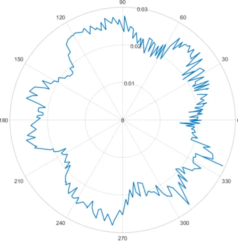
4.2.1

Torque-angle relation

As explained, the motor’s chambers cause non-linearities in torque. To deter-mine this relation, the Prony brake friction is increased to above the maximum motor torque, resulting in a static situation. Supply pressure is fixed to a value of 4 bar. The motor angle is then increased stepwise, manually, and measured by the encoder. In between, the load cell force is measured. This process is repeated until the motor has experienced two full rotations.

4.2.2

Motor speed and torque

Two important parameters of any rotary motor are its torque and rotational velocity. For electric motors, they are often related as shown in Figure 4.1. This curve is characteristic of a motor’s performance.

Figure 4.1:Example of a torque-speed relation for an electric motor.

A load cell is used to measure the friction torque applied by the Prony brake to the drive axle. Excess torque produced by the input pressure is converted to motor friction and acceleration. Under a constant input pressure, a (semi-) constant speed is eventually achieved.

To determine the torque-speed relation, a constant supply pressure is produ-ced. The friction torque absorbed by the Prony brake is varied by loosening or tightening the bolts. Any excess power produces by the motor is turned into rotational motion. Each configuration of the Prony brake results in a point on the torque-speed curve. Five different configurations, resulting in five different friction torques, are used, ranging from completely tightened to completely loosened. For each configuration, five measurements are used. This is done for pressures of 3 bar and 4 bar.

4.2.3

Pressure dynamics

Tubing between vane motor and valves inevitably introduces a delay into the system. Experiments are done by putting tubes of different lengths under pressure. After a set amount of time, pressure is released by exhausting air through the inlet. The time it takes the far end of the tube to reach the same pressure as the near end of the tube is determined for tubes of 1 m, 2 m, and 5 m.

In Section 3.3.1, it was theorised that adding an extra tube between the exhaust and downstream port would simplify the torque consideration, since no extra work would be done at the final portion of the cycle when the exhaust and downstream pressures are equal. The effectiveness of this tube is determined by exciting the vane motor with a chirp signal, and measuring the pressures at both the exhaust and downstream ports. If these pressures are exactly equal, no work is done by compression between the exhaust and downstream ports.

4.2.4

Dynamic response

Tubes of 5 m long are used, in the system configuration as designed in Chapter 3. Results are compared to results with tubes of 0.7 m.

Input and output The first step is to define the input and output of the vane motor system. A block diagram of the open-loop system is shown in Figure 4.2. The vane motor itself (Figure 4.3) has pressure difference∆P as input, and rotationφas output. Since pressure difference is linked to torque, which is proportional to the second time derivative of the output, this subsystem is expected to have a transfer function of the form _Js2₊1_ds+k.

The tubes introduce a delay in airflow. Flow at the tube’s end is dependent on tube length, as well as air and flow properties (Section 3.2.3). As pressure (difference) is the input for the vane motor, volume flow needs to be integrated. In the frequency domain, this integration acts as a low-pass filter.

Figure 4.2:Block diagram of open-loop vane motor system. Input voltage to proportional valve,up, being converted to a mass flow at the exhaust. This mass flow is integrated to determine exhaust pressure. The difference between this pressure and supply pressure produces a torque, which the vane motor converts to rotationφ.

Figure 4.3:Block diagram of the vane motor. Pressure difference∆Pis converted into torque by the chambers (see Section 3.2.2). This torque is then summed with friction and stiction torques, and divided by inertia to produce acceleration. This acceleration is then integrated twice into angleφ.

Regarding the valves, a transfer function of input voltageupto vane motor exhaust pressurePexis needed. From the datasheet supplied by manufacturer Camozzi, a graph is available showing a third-order relation between voltage and volume flow. Since the objective is to control the pressure at the outlet of the vane motor, an identification will be done on the transfer functionG(s) = _uφ(s)

p(s).

The directional valves where air passes through before entering the vane motor are only to switch direction of the air flow. The relevant dynamics at play here are in the switching time, which at 3 ms is probably faster than the system bandwidth.

Input voltage is measured by Beckhoff itself, which sends the command signal to the proportional valve, and is between 5V and 10 V. Rotation φis measured by the encoder (see also Figure 3.12).

Input signals Regarding the input signal, there are several options: multi-sine, frequency sweep (chirp), and PRBS. In a multi-multi-sine, harmonics of several different frequencies are used to excite the system (Figure 4.4). This input signal is suited to capture the response at certain frequencies, such as a (anti-)resonance. However, since this only portrays the response at certain frequencies, its use for representing a complete transfer function is limited.

Figure 4.4: Example of a multi-sine. The red, green, and blue harmonic sine waves are summed to produce an input signal which has frequency content at three distinct frequencies [53].

Another popular choice of input signal is a frequency sweep, or chirp signal (Figure 4.5). This signal excites a continuous band in the frequency spectrum, and so provides the response for this entire band. It can be used to get the system’s transfer function, provided all the relevant frequencies in the system are excited.

Finally, a Pseudo-Random Binary Signal (PRBS) is another type of input signal that is often seen in system identification. The PRBS switches between -1 and +1 in a (pseudo-) random fashion. A PRBS can be generated in multiple ways. MATLAB does this by using bit-shift operations, which produces a perfectly flat spectrum over the specified frequency range.

Both the chirp signal and the PRBS are used in this thesis, as they excite a broad spectrum of frequencies. In order to produce a consistent result, identifi-cation using a chirp signal is done as follows. Ten consecutive chirp signals are run with a small rest period of five seconds in between. Afterwards, the first two chirps are discarded to remove any transient effects. The other eight are averaged out to produce the final input/output data.

Sample time The sample time should be taken so that at least all of the rele-vant dynamics are captured. From the Shannon-Nyquist sampling theorem, the sample time should be at least twice as high as the highest frequency to be mea-sured. A lower limit for sample time stems from the type of state-space models that can be identified. In some model types, such as Auto-Regressive model with eXogenous input (ARX), the resulting model is determined by minimising error between real and predicted response at all frequencies [55]. If a high sampling rate is taken, the weighting will take into account high frequencies as well, where noise dominates. This can give a skewed representation of the system. This can be avoided by digital filters, which can reduce the sampling frequencies for identification.

To acquire the data a high sampling rate of 1 kHz is used, which is also the upper sampling frequency limit in Beckhoff. In order to lessen the focus on high-frequency behaviour, the signals are resampled to 500 Hz.

State-space models One representation of a Linear Time-Invariant system is a state-space model. In continuous-time, a state-space representation relates the states,x, of a system to their time derivatives by a set of first-order differential equations. A discrete-time implementation follows the following equations:

xk+1=Axk+Buk (4.1)

yk=Cxk+Duk, (4.2)

whereAis the system matrix,Bis the input matrix,uk is the current control input,Cis the output matrix,ykis the measured output signal and D(often empty) is the feedthrough matrix.

In order to identify a state-space model, one needs only to select a system’s order, which is equal to the dimensionality ofx. This means the system has does not need explicit definitions for the model equations, as the prediction error methods, discussed below, do. Once the order is set, the state-space parameters are optimised and one identified system is produced. This means that nuance in the delay of the system or the amount of zeroes cannot be explicitly defined.

Prediction error methods More distinction in system models can be applied by the so-called prediction error (PE) methods [55]. These methods attempt to fit a transfer function directly to the input/output data. While state-space

representations can be transformed to a transfer function, the result is not always optimal.

In PE methods, the outputyis related to the inputuand error/noisee:

y(t) =G(z)u(t) +H(z)e(t), (4.3)

for some transfer functionsG,H. These polynomials can be split into numerator and denominator, and the way this is parametrised determines the model type. For instance, in an AR(MA)X model, bothG(z)andH(z)share the same denominator, which means that the noise model follows the same dynamics as the system model. In ARMAX models,H(z)has its own numerator polynomial, which allows for some more nuance in identification. This compared to ARX models, where H(z)’s numerator is equal to 1. Output Error (OE) models, finally, follow the equationy(t) = B_F(_(zz−−11)₎u(t) +e(t), which assumesH(z) =1,

a white noise model.

The downside of PE methods is that a model structure must be defined befo-rehand. When using a structure that does not represent the system accurately, these methods can give misleading results.

Both state-space models and PE models are used in this thesis. For both type, input/output models of varying complexities are generated. For each fitted model, residual analysis is performed, which relates the expected model output to the real data and is a way to show the goodness-of-fit of a model.

4.3

Results

4.3.1

Torque-angle relation

Results on the non-linear torque-angle relation are discussed from both a mo-delling and a experiment point of view.

Model results In Figure 4.6, the modelled relation between rotation angle and pressure or torque is illustrated. In the top figure, the same expansion/compres-sion dynamics can be seen as in Figures 3.13 and 3.7. In the bottom figure, the sum of all vane torques (dashed line) can be seen to vary significantly with angle. This can be explained as follows. The highest difference in chamber pressures occurs whenever one chamber (A) reaches the exhaust. The previous chamber (B) will then have a pressure slightly lower than supply pressure (depending on geometry), thus producing a high torque. After this, chamber B expands, producing the negative slope in torque. Then the pressure in chamber B also drops to exhaust pressure, which explains the steep drop in torque.

Figure 4.6: Relation between angle and pressure (top) or torque (bottom) as modelled in Simulink.

Figure 4.7:Torque experienced by the Prony brake as a function of angle (blue). Radial axis shows torque in Nm, azimuthal axis shows angle in degrees.

Experimental results The relation between torque and angle is determined as described in Section 4.2. The results are plotted in Figure 4.7. It can clearly be seen that at certain intervals, the torque drops sharply. This happens every 72 degrees, which corresponds to the angle between two adjacent vanes (360o/5= 72o). Two full rotations are shown, with the angles transformed to the interval [0o, 360o].

4.3.2

Motor speed and torque

Torque is plotted against speed in Figure 4.8. A curve with a shape similar to that in Figure 4.1 can be seen, although the experimental data is quite scattered.

Figure 4.8:Torque as a function of angular velocity, for pressures of 3 and 4 bar. Markers indicate experiment results, lines a linear fit.

4.3.3

Pressure in tubes

Time to fill and evacuate the tubes is modelled in Section 3.2.2 as an attenuated, time-delayed response to an initial mass flow.

Figure 4.9:Reference and actual tube pressure as a function of time. Lt=5m,

dt=0.004m, ˙φ=100rad/s.