Are immigrants so stuck to the floor that the ceiling is irrelevant?

Are immigrants so stuck to the floor that the

ceiling is irrelevant?

Priscillia Hunt

No 838

WARWICK ECONOMIC RESEARCH PAPERS

Are immigrants so stuck to the ‡oor that the

ceiling is irrelevant?

Priscillia Hunt

February 2008

Abstract

In this paper, the immigrant-native wage di¤erential is explained through quantile regression estimations. Using repeated cross-sections of the British Labour Force Survey from 1993-2005, we analyse the returns to covariates across the conditional earnings distribution. We estimate a pooled model with an immigrant dummy and separate models for immigrants and natives of the UK. Our results show that the positive wage gap in favour of immigrants is attributed to those at higher quantiles. Returns to education and experience vary wider for natives than for immigrants. We decompose the wage gap in the Blinder-Oaxaca framework and apply quantile regression techniques to see if immigrants simply have more viable labour market characteristics than natives or if there is a preference for immigrant workers (reverse discrimination). Our …ndings suggest immigrants should actually be earning more and there is su¢ cient evidence of discrimination. This …nding is, however, not symmetric across the conditional wage distribution and immigrants at the bottom face more discrimination than those at the top.

Keywords: immigration, wage di¤erential, quantile regression, Blinder-Oaxaca decomposition

JEL Classi…cation: J31, J61, J71

1_{Address: Department of Economics, University of Warwick, Coventry CV4 7AL,} UK. Email: [email protected]

1

Introduction

When immigrants enter a new country to settle and work, there is a period of integration in which the foreign-born must learn a new language, job opportu-nities, methods of transportation, banking system, laws, and cultural norms. The ability to assimilate into a new economy is important for the economic success of both the existing and next generation of workers. Until recently, im-migration to the United Kingdom was of relatively little economic signi…cance because Britain was primarily a region of net emigration (Hatton (2005)). In the last few decades, there has been greater in-migration and less out-migration, resulting in more concern about the state of Britain’s labour market (O¢ ce of National Statistics 20053).

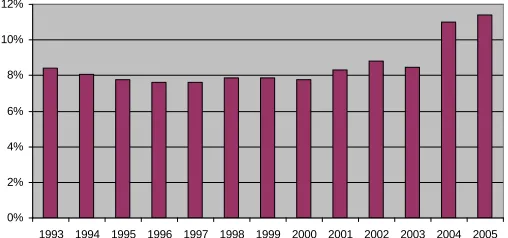
The proportion of foreign-born workers in Britain remained roughly 8 per-cent in the early 1990’s. As shown in Figure 1, there was a sharp increase to roughly 11 percent in 2004 and 2005. This substantial increase coincides with the EU enlargement of 20044_{, thus we might think the recent increase is mostly} due to the heightened ‡ow of Eastern European workers.

Figure 1: Proportion of NonUK-born in UK Labour Force, LFS 1993-2005

0% 2% 4% 6% 8% 10% 12%

1993 1994 1995 1996 1997 1998 1999 2000 2001 2002 2003 2004 2005

Looking at Table 1, we determine region of origin variation for the increased proportion of foreign-born. We see the increase is in fact e¤ectively European in 2005 (+2.46%). There is also some growth, in proportion, from 2004 to 2005 for individuals from China/Hong Kong (+1.02%) and India (+1.89%). For 2004, the distribution for region of origin remained fairly similar to 2003, except we …nd a drop in workers from the Old Commonwealth & United States (-1.15%). Table 1 illustrates the proportion of immigrants in public- and private-sector employment, thus excluding the self-employed, and there may be origin di¤erences that a¤ect the wage pro…le for immigrants.

3_{http://www.statistics.gov.uk/cci/nugget.asp?id=1311}

4_{Cyprus, the Czech Republic, Estonia, Hungary, Latvia, Lithuania, Malta, Poland,}

Ireland

Caribbean & West

Indies China/

HK Europe India

Pakistan/ Bang.

Old Common-wealth &

US

Rest of the World

1997 13.85% 5.15% 1.42% 21.31% 8.88% 4.62% 12.26% 32.50%

1998 11.79% 5.83% 1.66% 20.11% 10.40% 5.69% 15.26% 29.26%

1999 11.65% 5.12% 1.09% 20.34% 10.25% 5.43% 15.37% 30.75%

2000 11.29% 4.01% 0.89% 19.02% 9.96% 4.61% 16.05% 34.18%

2001 9.02% 4.37% 1.89% 22.85% 8.73% 5.24% 16.16% 31.73%

2002 7.70% 3.65% 1.49% 20.41% 7.30% 5.00% 19.05% 35.41%

2003 8.16% 4.23% 1.96% 22.05% 9.37% 4.23% 18.13% 31.87%

2004 8.65% 4.56% 2.04% 22.01% 9.28% 4.25% 16.98% 32.23%

2005 5.45% 2.53% 3.06% 24.47% 11.17% 4.26% 16.36% 32.71%

Source: Author's LFS Sample, 1997-2005, Employed Men only

Table 1: Percentage of Employed Immigrants by Region of Origin from 1997-2005

Success in the labour market is determined, in part, to the level of educa-tion obtained. Figure 2 shows the educaeduca-tional attainment of immigrant and native workers. It is clear from this illustration that the NonUK-born workers in Britain have relatively more education. Immigrants and natives have roughly the same proportions, 21% and 17% respectively, in the middle education group (leaving age of 17-18yrs). There are stark di¤erences in the lower and higher ed-ucation groups. 36.2% of immigrants are in the lowest eded-ucation group (leaving age of 16 yrs or less) and 65.5% of natives are in this lowest education group. Nearly 18% of natives and 43% of immigrants are in the highest education group (leaving age of 19+ yrs). This polarisation of education for immigrants indi-cates negative and positive observed selection and a potential source of greater wage disparity for immigrants than natives. Since the rate of immigration is increasing, this polarisation will have an e¤ect on overall wage equality.

Figure 2: Education Distribution for Employed Males of Britain, LFS 1993-2005

0.00 0.10 0.20 0.30 0.40 0.50 0.60 0.70

Less than 17yrs 17-18 yrs 19+ yrs

Education Leaving Age

F

requenc

y

UK-born

NonUK-born

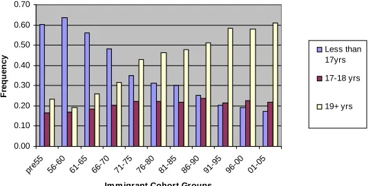
and an upward trend of highly-educated immigrant workers. The proportion of immigrants leaving school at 17 or 18 has been constant. It is beyond the scope of this paper to suggest why this occurred, however, it would be interesting to …nd what policies and/or economic relationships prompted this trend.

Figure 3: Density of Education leaving age for Immigrant cohorts in the LFS

0.00 0.10 0.20 0.30 0.40 0.50 0.60 0.70

pre55 56-60

61-65

66-70

71-75

76-80

81-85

86-90

91-95

96-00

01-05

Im m igrant Cohort Groups

Fr

e

que

nc

y Less than_17yrs

17-18 yrs

19+ yrs

The di¤erences in observed characteristics and returns to those character-istics may di¤er across the income distribution for natives and immigrants. Martins and Pereira (2003) perform quantile regression analysis to evaluate conditional returns to education across the earnings distribution and it appears that higher-ability individuals, or those earning a higher hourly wage condi-tional on education and experience, gain more from education. This result was particularly strong for Britain where OLS estimates suggested a 0.083 premium on education, yet the di¤erence between returns for those in the 10th and 90th percentiles of the earnings distribution are respectively, 0.045 and 0.092. With the …ndings of Manacorda, Manning, and Wadsworth (2006) in which immi-grants depress the wages of other immiimmi-grants, we should …nd the wage gap for immigrants is smaller than for natives. Conversely, the unobserved skills of high-skilled immigrants may be greater than those for low-skilled in such a way that does not exist between low- and high-skilled natives. If we …nd smaller wage gaps for immigrants than for natives across their respective earn-ings distributions, then the impacts demonstrated by Manacorda et al (2006) are economically signi…cant.

immigrant-native wage gap. The results allow us to discuss the implications of work and wage inequality in Britain.

The remainder of this paper is organised as follows. Section 2 surveys liter-ature looking at sources of immigrant-native wage gaps in Britain and the US. Section 3 introduces our modelling and estimation strategy. Section 4 describes the data set and presents summary statistics. We display our results in Section 5 and the …nal section concludes with policy implications and areas for further research.

2

Literature

The theoretical framework for immigrant earning pro…les was developed in Chiswick (1978, 1980), which argues immigrants cannot immediately compete with natives because they lack human capital exclusive to the destination. As time in the host country labour market progresses, outcomes of foreign-born workers assimilate towards their native counterparts. Chiswick (1980) …nds 6 percent wage advantage for white immigrants and 19 percent lower earn-ings for nonwhite immigrants in the British General Household Survey of 1972. Chiswick’s (1980) work revealed a severe pitfall to estimating wage di¤erentials using cross-sectional data- immigrant cohorts changes over time and the ’snap-shot’aspect of cross-sections misrepresents the earnings immigrants may expect. In this paper, we include cohort dummies and utilise a repeated cross-sectional data set in order to correctly estimate foreign-born earnings pro…le.

Since the work of Chiswick (1980), many authors (see the Home O¢ ce report (1999)) have investigated immigrant economic outcomes by ethnicity, race, co-hort, and intent of entry to uncover what factors put these immigrants at a wage advantage or disadvantage. Bell (1997) examines data from the General House-hold Survey for the period 1973-1992 and …nds UK immigration policy attracted higher-skilled immigrants, even though it did not consider socio-economic char-acteristics for entrance. White immigrants have an initial advantage over native whites, which eventually dissipates. He also …nds ethnic minority immigrants have an initial wage disadvantage that slowly lessens, but does not disappear as they assimilate. Clark and Lindley (2006) examine the 1993-2002 Labour Force Survey and distinguish between education and labour market immigrants to …nd there is a great deal of variance in labour market success rates based on ethnic di¤erences. There is some indication non-white immigrants have lower earnings due to unemployment rates upon entry (i.e. "scarring e¤ect"). Using the same data set, Dustmann, Fabbri, Preston, and Wadsworth (2003) estimate wage equations for UK- and NonUK-born whites and nonwhites. They …nd the largest wage gap is between UK whites and nonwhites, whilst the wage di¤er-ential between UK-born whites and nonwhite immigrants is relatively muted. This paper contributes to the literature by reporting the immigrant-native wage gap across the conditional earnings distribution.

the wage structure changed over the last decade and this harmed some work-ers whilst helping othwork-ers. Manacorda, Manning, and Wadsworth (2006) use the British General Household Survey (GHS) and British Labour Force Survey (LFS) to estimate a CES production function and assess changes to the wage structure. They …nd the rise in immigration has changed Britain’s wage struc-ture and depressed the earnings of immigrants relative to native-born. The wages of native-born workers relative to immigrants can vary over time even with …xed levels of demand and supply and authors indicate immigrants only a¤ect the wages of other immigrants. Since Card and Lemieux (2001) conclude that the return to university education is sensitive to the relative supply of uni-versity graduates and because data indicates immigrants are better-educated than natives, immigration will have reduced the return to education. Through simulation techniques, Manacorda et al. (2006) determine imperfect substi-tutability and small immigrant sizes eliminated the immigrant e¤ect on native wages. The Blinder-Oaxaca decomposition allows us to separate the di¤erences in native and immigrant earnings due to di¤ering characteristics and to discrim-ination (Blinder (1973); Oaxaca (1973)).

3

Empirical Strategy

3.1

Modelling

The competitive model framework assumes there are so many …rms that no sin-gle …rm has enough demand to a¤ect wages. Pro…t-maximising …rms set prices of labour (wage) equal to marginal productivity of labour, since any more or less reduces pro…ts. Typical skills contributing to an individual’s productivity are schooling and experience, however, levels of education and years of experience alone do not induce technological progress nor build customer relationships. Be-havioural traits also contribute to the manufacture and sale of …rm goods and services and in‡uence the working environment. Thus, …rms are willing to pay a premium for positive unobservable qualities as well. Green, Machin, and Wilkin-son (1998) learn that British employers consider motivational, attitudinal, and social skills an important contributing factor to the ’skills shortage’. Moreover, these attributes have an ethnic dimension in which Bauder (2006) …nds clear di¤erences in work attitudes between national origin groups. Hence, observable and unobservable qualities are important factors to consider in the analysis of wage disparities between natives and immigrants. All models include standard variables for human capital (i.e. years of education, potential experience), indus-try and region dummies, and personal characteristics (i.e. Non-white, Married status, Non-English as …rst language).5 The single model with a foreign dummy variable is the following:

wage=f(EXP; EDY RS; M IG; N ON W; M ARC; EN G; IN DU S; U RESM C):

In order to develop a framework of comparison, we must understand what factors enter the wage integration process and make assumptions about how it all works. The basic conjecture is assimilation in Britain occurs over time (Dustmann et al (2003)). The more time workers spend in the host country, the more they adapt to their environment. Thus, we include a variable account-ing for the number of years spent in the host country. We do not presume, however, the speed of adjustment is similar for all immigrants. An important consideration for integration in the UK labour market is country of origin. Due to historical ties, many countries are relatively similar, such as the Ireland and UK, and skills will easily transfer from home to host country. High degrees of skill transferability reduces assimilation time of the worker and improves overall earnings. Generally, immigrants can easily transport their skills if they move to a country that speaks the same language. We use national language to proxy for skill transferability since English-speaking immigrants will gather more in-formation about job prospects and communicate their abilities more e¤ectively to employers and customers. To estimate separate models for immigrants and natives, there are variables in the immigrant that clearly cannot be included for natives. The model for natives is as above and for immigrants includes covariates accounting for the assimilation process:

wage=f(EXP; F ORx; EDY RS; U Ked; N ON W; M ARC; EN G; IN DU S; U RESM C; REGOB; AGEAIM; Y RSSIN).

Lastly, we estimate a decomposition model established by Blinder-Oaxaca (Blinder (1973); Oaxaca (1973)). The Blinder-Oaxaca decomposition is a useful tool to estimate the nature of our immigrant-native wage gap . The basic idea is to break down the earnings gap between two groups as the di¤erence in observable characteristics and di¤erence in the bene…ts to those characteristics. Letk represent natives andm for immigrants and suppose the wage equation takes the form:

lnwk_i = kxk_i +"n_i (1) where wk

i are wages for a native individual i and xki is a vector of observable

characteristics for a native individuali, k denotes the vector of parameters to be estimated and"n_i is a normally distributed disturbance term with zero mean. In the same fashion, we will have for immigrants:

lnwm_i = mxmi +"mi . (2)

The di¤erence of these two equations is:

lnwk_i lnwm_i = ( kxk_i mxm_i ) + ("k_i "m_i ). (3) We can calculate the di¤erence between the mean wage logarithms for the two groups and add and subtract^kxm_{to get:}

lnwm lnwk =^k(xm xk) + (^m ^k)xm, (4)

whereE("k_{) =E("}m_{) = 0. The …rst term of the decomposition,} ^k_(xk _xm_),

indicates the "explained" component of wage di¤erences between natives and immigrants or the part of the wage gap which can be attributed to di¤erences in average observable characteristics of the individuals in each group. The second term,(^m ^k)xm_{, can be interpreted as the "unexplained" component of the}

wage gap in which immigrants experience a di¤erence in returns to characteris-tics due to mere association with the ’immigrant group’.

Clearly, we could add and subtract ^mxk instead, which is the crux of the standard ’index number’ problem (see Oaxaca and Ransom (1999)). It is not a problem in the summation of the wage gaps, but we will …nd di¤erent es-timates of the wage gap at each covariate when there are dummy covariates. We, therefore, perform estimations with natives as the reference group, then immigrants as the reference group, and lastly, as suggested in Cotton (1988), we assign population proportion weights. Results for natives as the reference group are presented in the body of the paper.6

3.1.1 Participation Selection

As with any wage equation, there is a danger of selectivity bias where only those who are working are included in the sample. Ideally, we would like to include the unemployed who are e¤ectively choosing zero wages, but are left out of the model. There are no parental variables in the LFS and we were not able to …nd a suitable instrument. Thus, we conclude that there is potential upward bias in our parameter estimates should the participation e¤ect be signi…cant.

3.2

Estimation

3.2.1 Quantile Regression

In addition to standard OLS estimations, we take a further step to encapsu-late any unobserved heterogeneity in the individual wage equations. Following Koenker and Bassett (1978) and Buchinsky (1998), we let(yi; xi), i= 1; :::; N,

be the LFS random sample of the UK population. xi is a K 1 vector of

observable characteristics to individuali and yi is the dependent variable, log

real hourly wages. The conditional quantile ofyi, conditional on the vector of

explanatory variablesxi, isQuant (yijxi) = xi . We assume the conditional

error term at each quantile isQuant (u ijxi) = 0. Then, the model is simply

yi=xi +e i (5)

The estimation process is similar to OLS in that parameter estimates are derived through minimisation of the errors. OLS measures least distance for the sum of the squared errors, whilst QR measures least distance of weighted absolute values of the error. Generally speaking, the ‘weights’ are percentiles that can take on the various values for which the researcher is interested. For example, the weighted least absolute deviation estimator for the median regres-sion is the result when =:5. An advantage of the quantile regression approach is that outliers are not given extra weight of the OLS procedure, which squares the errors. We will see that this is particularly important in terms of the LFS sample, which has some extreme values reported for weekly wages and weekly hours worked.

Since quantile functions do not specify how variance changes are linked to the sample mean, it is not necessary to specify the parametric distributional form of the error. Although as we indicated above, the error term at each quantile is zero. Thus, the thquantile regression estimator for is de…ned as:

min

8 < :

X

i:y xi

jyi xi j +

X

(1 )

i:y<xi

jyi xi j

9 =

; (6)

3.2.2 Blinder-Oaxaca QR Decomposition

and Mata (2005). The estimation procedure involves generating the UK-born log wage density that would arise if natives were given immigrant’s labour mar-ket characteristics but continued to be “paid like natives”(i.e. ^kxm). In order to estimate this marginal density, Machado and Mata (2005) indicate we …rst …nd which quantiles that should be estimated. Then, we estimate parameters in each of those quantiles for immigrants and natives separately. Next, we must randomly draw natives (with replacement) to determine the distribution of covariates and use this with the estimated coe¢ cients in each quantile to determine the counterfactual density. There are several methods we can choose to perform this …nal step. The di¤erence in approaches come down to whether to construct average characteristics in each quantile,xm_{, (Machado and Mata}

(2005), Albrecht et al. (2003)) or average characteristics of the whole sample, xm_{, (Montenegro (2001), Blaise (2005)). We follow Machado and Mata (2005),}

which entails using the distribution of immigrant characteristics to decompose the wage gap at quantiles of interest. In practice, this requires performing a bootstrap sample of size 100 and ordering each observation into percentile one, percentile two, and so forth. After 500 repetitions, we utilise covariate means at percentiles, or quantiles, of interest in the decompositions. Formally, the steps are the following:

1. Draw on the native data from the LFS to estimate the quantile regression coe¢ cient vectors,^k, for =:10; :25; :50; :75; :90.

2. Make 100 draws at random with replacement from the immigrant data from the LFS and sort by earnings.

3. Repeat 500 times to obtainxm for =:10; :25; :50; :75; :90

4. The counterfactual density is then generated as_fln ^w = ^kxm_g.

We follow Machado and Mata (2005) almost identically, except they suggest a …rst step should be to determine the quantiles, j [0;1] for j = 1; :::n. We

predetermine the quantiles of interest as 0.10, 0.25, 0.50, 0.75, and 0.90. We want to eliminate any possibilities of violating the assumption of monotonicity in the estimated conditional quantile functions and ensure enough variation across the subsamples. Koenker and Bassett (1982) argue the less dense are the set of

0_{s in[0;1], the less likely we violate this presumption. It is also the case that}

the larger the sample size becomes, the less likely one violates monotonicity; however, the immigrant small size is arguably still small. Hence, we estimate at these …ve quantiles. The Blinder-Oaxaca decomposition for quantile regression becomes:

lnwm lnwk =^k(xm xk) + (^k ^m)xm.

4

Data

Autumn (September-November), and Winter (December-February). Each quar-ter samples 125,000 individuals from approximately 60,000 households. Not all questions are posed to a household at once. The questions are posed over …ve successive quarters, which are called ’waves’. Therefore, in each quarter 12,000 households are in their wave 1, 12,000 are in wave 2, etc. The LFS is released quarterly and there are variables indicating the interviewee’s wave, as well as the quarter and year the individual entered the survey. Quarters of the LFS were seasonal until January 2006; the survey was then switched to calendar-quarters in order to ful…l European Union regulations. The survey has been carried out annually in its current form since 19837_{; however, earnings information is only} available since 1992. The earnings question is asked in wave 5 from 1992 on-wards and then also in wave 1 from 1997 onon-wards. For consistency, we use wave 5 wages whenever possible. We only use wave 1 earnings for those persons with positive wages in wave 1 and non-response in wave 5. When we in‡ate wages, we use the index corresponding to the year and quarter when the respondent gave their earnings details.8 Wages are reported in terms of weekly earnings, so we derive hourly wages by dividing (gross) weekly earnings into weekly hours worked. To account for in‡ation and determine real wages, we use the UK Re-tail Price Index (RPI)9_{. We use 2005Q4 prices as the base period to in‡ate all} prior earnings observations. We pool cross-sections of the LFS from 1993Q1 to 2005Q4. The data used for this estimation includes men aged 16-64 in full-time employment. Earnings are not reported for the self-employed.

4.1

Summary Statistics

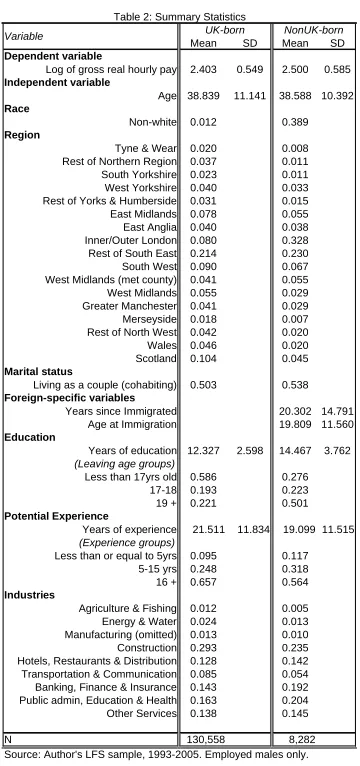
In Table 3, we present a summary of statistics characterising the sample we use for wage analysis. The data is from 1993 to 2005 and descriptive statistics are aggregated data of individual level responses from the LFS data set. Results show that foreign-born workers earn more than UK-born, £ 14.51 and £ 12.85 re-spectively. Foreign-born workers are on average the same age as native workers, roughly 38 years old. Average age at immigration is 19 years old and average years in the UK is 20 years. There are signi…cantly more non-whites in the immigrant population than in the native population. Less than 2% of working age, employed males born in the UK are non-white, whilst 39% of the immi-grant workforce are non-white. The geographical dispersion of UK-born workers is much greater for natives than immigrants. The greatest regional concentra-tion of UK-born working males is in the South East (21%), 2-9% concentraconcentra-tion in the other regions of England, and 10% living in Scotland. Immigrants, on the other hand, are highly concentrated in London (33%) and the South East (23%). Roughly the same proportion of natives and immigrants are married or living together as a couple, 50% and 54% respectively.

7_{The LFS was carried out on a biennial basis from 1973 to 1983.}

8_{We do not use the year and quarter in the survey because that relates to the period in}

which the respondent entered the survey.

Mean SD Mean SD

Dependent variable

Log of gross real hourly pay 2.403 0.549 2.500 0.585

Independent variable

Age 38.839 11.141 38.588 10.392

Race

Non-white 0.012 0.389

Region

Tyne & Wear 0.020 0.008

Rest of Northern Region 0.037 0.011

South Yorkshire 0.023 0.011

West Yorkshire 0.040 0.033

Rest of Yorks & Humberside 0.031 0.015

East Midlands 0.078 0.055

East Anglia 0.040 0.038

Inner/Outer London 0.080 0.328

Rest of South East 0.214 0.230

South West 0.090 0.067

West Midlands (met county) 0.041 0.055

West Midlands 0.055 0.029

Greater Manchester 0.041 0.029

Merseyside 0.018 0.007

Rest of North West 0.042 0.020

Wales 0.046 0.020

Scotland 0.104 0.045

Marital status

Living as a couple (cohabiting) 0.503 0.538

Foreign-specific variables

Years since Immigrated 20.302 14.791

Age at Immigration 19.809 11.560

Education

Years of education 12.327 2.598 14.467 3.762

(Leaving age groups)

Less than 17yrs old 0.586 0.276

17-18 0.193 0.223

19 + 0.221 0.501

Potential Experience

Years of experience 21.511 11.834 19.099 11.515

(Experience groups)

Less than or equal to 5yrs 0.095 0.117

5-15 yrs 0.248 0.318

16 + 0.657 0.564

Industries

Agriculture & Fishing 0.012 0.005

Energy & Water 0.024 0.013

Manufacturing (omitted) 0.013 0.010

Construction 0.293 0.235

Hotels, Restaurants & Distribution 0.128 0.142

Transportation & Communication 0.085 0.054

Banking, Finance & Insurance 0.143 0.192

Public admin, Education & Health 0.163 0.204

Other Services 0.138 0.145

N 130,558 8,282

UK-born NonUK-born

Table 2: Summary Statistics

Source: Author's LFS sample, 1993-2005. Employed males only.

Variable

Table 2 reports immigrants have relatively more workers leaving education at 19 years old or later (50%) than natives (22%). Conversely, natives are more concentrated (59%) in the lowest education group than natives (28%). Immigrants and natives have similar proportions, 19% and 22% respectively, in the middle education group of 17-18 years leaving age. Regarding years of experience, immigrants have less overall than natives. Nearly 66% of natives are in the highest experience group, whilst 56% of immigrants are within this category.

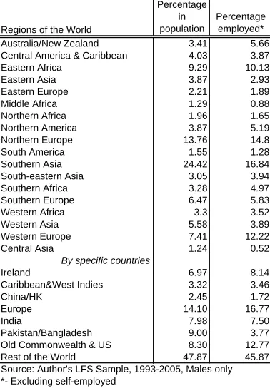
In Table 3, we present the distributions for the regions of birth10 _and coun-tries of birth for immigrants in the UK for 1993-2005. The …rst column illus-trates the proportion of immigrant males in the UK immigrant male population. The second column presents the proportion of immigrant males in the UK

grant work force. By contrasting these two tables, we observe ethnic di¤erences in employment and we …nd there are several signi…cant ethnic di¤erences. The top of the table demonstrates quite clearly that South Asian males are a sig-ni…cant proportion of the population (24%), but they are less prevalent in the labour force (17%). By disaggregating the immigrant population into areas of interest11_{, we …nd the weak employment propensities for South Asian males} are mostly due to Pakistanis and Bangladeshis. This con…rms reports of high self-employment propensities and/or low participation rates for Pakistani and Bangladeshi males (Dustmann et al (2005)). The top part of the table illus-trates lower proportions in the second (employed) column for Central American & Caribbean, Eastern Asia, Eastern Europe, Middle Africa, Northern Africa, South America, South Asia, Southern Europe, Western Asian, and Central Asia. It is beyond of the scope of this paper to suggest why this exists, however, one must consider these results do not include the self-employed or those outside legal employment.

Regions of the World

Percentage in population

Percentage employed*

Australia/New Zealand 3.41 5.66

Central America & Caribbean 4.03 3.87

Eastern Africa 9.29 10.13

Eastern Asia 3.87 2.93

Eastern Europe 2.21 1.89

Middle Africa 1.29 0.88

Northern Africa 1.96 1.65

Northern America 3.87 5.19

Northern Europe 13.76 14.8

South America 1.55 1.28

Southern Asia 24.42 16.84

South-eastern Asia 3.05 3.94

Southern Africa 3.28 4.97

Southern Europe 6.47 5.83

Western Africa 3.3 3.52

Western Asia 5.58 3.89

Western Europe 7.41 12.22

Central Asia 1.24 0.52

By specific countries

Ireland 6.97 8.14

Caribbean&West Indies 3.32 3.46

China/HK 2.45 1.72

Europe 14.10 16.77

India 7.98 7.50

Pakistan/Bangladesh 9.00 3.77

Old Commonwealth & US 8.30 12.77

Rest of the World 47.87 45.87

Table 3: Region of Birth Distribution for UK Immigrants

Source: Author's LFS Sample, 1993-2005, Males only *- Excluding self-employed

1 1_{From 1993-1996, the LFS limits responses for ’origin of birth’ to- Ireland, Hong Kong,}

5

Results

5.1

Pooled Regressions with Foreign Dummy

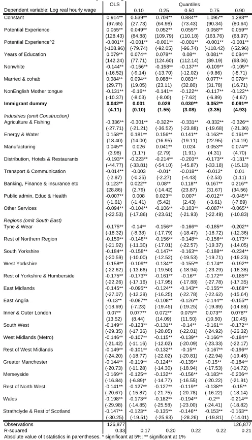
This model demonstrates the "return to being foreign", holding all else equal. Results are displayed in Table 9 in Appendix B. OLS regression estimates in-dicate a 0.042 premium to foreign status; however, it is clear from the QR estimates that these returns are not homogeneous across the conditional wage distribution. In the 10th percentile, coe¢ cients are not statistically di¤erent from zero. In the 25th percentile, the coe¢ cient on foreign status increases to 0.029, but is still not statistically signi…cant. At the median, results become signi…cant and the coe¢ cient is +0.30 log point. This increases to 0.052 and 0.091 log points for the 75th and 90th percentiles, respectively. Therefore, we can say that relative to the low-ability immigrants, the high-ability immigrants encounter wage gains associated with being an immigrant. Put another way, workers of low-ability earn the same whether an immigrant or native. Higher ability workers earn more as an immigrant than a native.

We …nd the years of education and experience increase only slightly across the wage distribution. The coe¢ cient on nonwhite varies considerably from the lowest to highest quantiles. The average e¤ect appears to be a -0.144 log point decrease in wages, whereas the e¤ect for those in the 10th percentile is -0.156 and in the 90th percentile it is less at -0.105 log points. We separate out the language e¤ect from migrant status and …nd a decreasing negative e¤ect across the conditional distribution. The impact of a di¤erent mother tongue than English is -0.16 log point reduction in wages for the least (10th percentile) able workers and approximately -0.12 for the most (50th, 75th, and 90th percentile) able workers. There is evidence, therefore, the highest ability workers are able to persevere through the language barrier somewhat, but not entirely. It has a real negative impact on the wage potential of even the most ambitious and loyal workers.

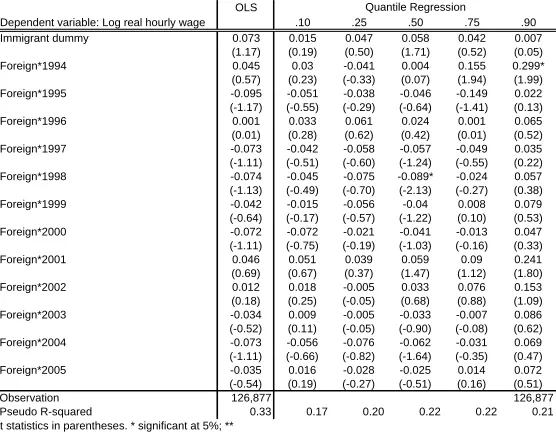
The second regression model includes an interaction term between foreign status and year dummies. We can see in Table 4 below (full results are in Table 10 of Appendix B), the immigrant e¤ect becomes statistically insigni…cant with the inclusion of interaction terms. The interaction terms are the e¤ect of being foreign in a particular year compared to being foreign in 1993. All are statistically insigni…cant and fail to show any pattern or trend for the signs. The positive e¤ect of ’foreignness’we found in the …rst model (0.042 log points) remains the case here (0.073 log points), but becomes statistically insigni…cant.

Dependent variable: Log real hourly wage .10 .25 .50 .75 .90

Immigrant dummy 0.073 0.015 0.047 0.058 0.042 0.007

(1.17) (0.19) (0.50) (1.71) (0.52) (0.05)

Foreign*1994 0.045 0.03 -0.041 0.004 0.155 0.299*

(0.57) (0.23) (-0.33) (0.07) (1.94) (1.99)

Foreign*1995 -0.095 -0.051 -0.038 -0.046 -0.149 0.022

(-1.17) (-0.55) (-0.29) (-0.64) (-1.41) (0.13)

Foreign*1996 0.001 0.033 0.061 0.024 0.001 0.065

(0.01) (0.28) (0.62) (0.42) (0.01) (0.52)

Foreign*1997 -0.073 -0.042 -0.058 -0.057 -0.049 0.035

(-1.11) (-0.51) (-0.60) (-1.24) (-0.55) (0.22)

Foreign*1998 -0.074 -0.045 -0.075 -0.089* -0.024 0.057

(-1.13) (-0.49) (-0.70) (-2.13) (-0.27) (0.38)

Foreign*1999 -0.042 -0.015 -0.056 -0.04 0.008 0.079

(-0.64) (-0.17) (-0.57) (-1.22) (0.10) (0.53)

Foreign*2000 -0.072 -0.072 -0.021 -0.041 -0.013 0.047

(-1.11) (-0.75) (-0.19) (-1.03) (-0.16) (0.33)

Foreign*2001 0.046 0.051 0.039 0.059 0.09 0.241

(0.69) (0.67) (0.37) (1.47) (1.12) (1.80)

Foreign*2002 0.012 0.018 -0.005 0.033 0.076 0.153

(0.18) (0.25) (-0.05) (0.68) (0.88) (1.09)

Foreign*2003 -0.034 0.009 -0.005 -0.033 -0.007 0.086

(-0.52) (0.11) (-0.05) (-0.90) (-0.08) (0.62)

Foreign*2004 -0.073 -0.056 -0.076 -0.062 -0.031 0.069

(-1.11) (-0.66) (-0.82) (-1.64) (-0.35) (0.47)

Foreign*2005 -0.035 0.016 -0.028 -0.025 0.014 0.072

(-0.54) (0.19) (-0.27) (-0.51) (0.16) (0.51)

Observation 126,877 126,877

Pseudo R-squared 0.33 0.17 0.20 0.22 0.22 0.21

t statistics in parentheses. * significant at 5%; **

Table 4: OLS & QR Results of Pooled Model, with Immigrant-Year interactions

OLS Quantile Regression

5.2

Regressions by Nativity

OLS estimates indicate a 0.043 log point increase in each additional year of work experience. This ranges steadily from 0.031 log points for the bottom 10th per-centile of workers to 0.055 for the top 10 perper-centile of workers. We …nd a 0.061 log point premium to each additional year of education.

The in‡uence of personal characteristics on earnings varies only slightly across the conditional wage distribution. Holding all else equal, OLS estimates a -0.069 log point reduction in wages for nonwhites. This negative e¤ect bounces around across the conditional distribution, ranging from estimates of -0.063 to -0.080 log points. The positive e¤ect of the marriage/cohabiting variable de-creases across the conditional earnings distribution. There is an average e¤ect of 0.086 log point increase on real hourly wages, as determined through OLS. Quantile regression tells us this e¤ect is actually more positive at the lower quantiles- 0.096 and 0.088 log points at the 10th and 25th quantiles, respec-tively and 0.79 log points at both the 75th and 90th quantiles.

The impact of working in particular industries, compared to manufacturing, is heterogenous across the conditional wage distribution. Construction yields greater returns for those with high unobservable skills, 0.075 log points at the 90th quantile. Estimates show returns are not signi…cantly di¤erent from zero (i.e. 0.027, yet statistically insigni…cant) at the 10th quantile. Similarly, returns are consistently less and less negative across the distribution for workers in Distribution, Hotels & Restaurants. Workers in Banking, Finance & Insurance at the top of the distribution earn 0.211 log point premium, whilst those at the bottom earn 0.015 log point premium for working in Banking rather than Manufacturing. We …nd the most striking di¤erences across the distribution to be in Public Administration, Education & Health. OLS estimates an average decrease in earnings as -0.011 log points in real hourly wages, compared with average Manufacturing wages. Rates of return are not signi…cantly di¤erent from zero or positive below the 50th quantile. There is a strong depressive e¤ect on wages for high ability individuals, -0.014 and -0.046 log points at the 75th and 90th quantiles.

Regarding the regions of inhabitancy in the UK, all estimates are in com-parison to the South East. Only London yields a positive e¤ect on hourly wages relative to the South East. Quantile regression analysis indicates the average positive e¤ect from OLS, 0.073 log point, is an accurate estimate since coe¢ -cients across the quantiles range from 0.074 to 0.082.

additional school year, which is nearly identical to the …ndings of Martins and Pereira (2003) for the entire British labour force. Unlike their results, we …nd the highest ability workers do not earn such a premium from education (0.076 log points at the 90th percentile). These results appear to con…rm the …ndings that immigrants compress the earnings of other immigrants, particularly at the top of the conditional earnings distribution. The dummy variables for foreign experience and UK education produce some interesting results. In particular, individuals with some education in a British institution have greater wages than those who do not, as else equal. Although the estimates are weakly signi…cant, the greatest return to UK education is at the median (0.079 log points). This falls to roughly a 0.60 log points at the 25th, 75th, and 90th percentiles. In-terestingly, for those in the 10th percentile, the return to UK education is far below the other quantiles (0.013 log points). Perhaps more intriguing is the …nding that returns switch from negative to positive across the quantiles for the possession of foreign experience.

The in‡uence of personal characteristics on immigrant earnings varies only slightly across the conditional wage distribution. OLS estimates a 0.192 re-duction in wages for nonwhite immigrants relative to white immigrants, ceteris peribus. This negative e¤ect diminishes across the conditional distribution, but does not dissipate entirely. The marriage/cohabiting variable is correctly esti-mated through the OLS regression technique for those in the 10th, 25th, and 75th percentiles (0.07 log points). It appears the highest ability workers do not earn a wage premium through marriage or cohabitation. OLS estimates a depressive e¤ect, -0.098 log point, of immigrating from a nonEnglish-speaking versus an English-speaking country. The impact is actually greater for the low-est ability individuals, -0.114 at the 10th percentile, and lessens to -0.083 log points for the highest ability individuals.

We are interested in the impact of working in particular industries and re-gions because immigrants are more concentrated in certain sectors and areas of Britain than natives. Relative to manufacturing, OLS results indicate a pre-mium to working in Energy & Water (0.161 log point) and Banking, Finance, & Insurance (0.196 log point) sectors. Quantile regression estimates break down the returns to these industries and we …nd dissimilar results between the two industries. Within the Energy & Water industry, the 10th, 25th, and 50th percentile workers earn more than those at the top of the conditional distrib-ution. For those in Banking, Finance, & Insurance, we …nd increasing wages across the conditional wage distribution. This is not alike the results we would …nd for public-private sector or union-nonunion quantile estimates in which the protection of governments and unions increase the wages of the lowest-ability individuals and private …rms reward high ability workers.

comparison in OLS results of immigrants and natives.

5.3

Blinder-Oaxaca Decomposition

5.3.1 OLS

The pooled model and separate estimations make it clear there is a wage pre-mium to immigrant status, yet di¤erential returns to characteristics for immi-grants and natives. We are still unclear about the source of wage advantage and disadvantages. We still need to illustrate whether the observed di¤erential treatment of immigrants and natives in the workforce is due to labour market di¤erences or discrimination. We utilise OLS and QR techniques to the break down of equation(4), otherwise known as the Blinder-Oaxaca decompositions.

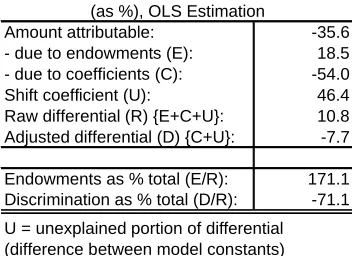
In Table 5, we present OLS estimates of the decompositions, which consists of running regressions on each of the groups and then comparing results in the Blinder-Oaxaca framework. The table illustrates di¤erences in labour market characteristics (E) and rewards to those characteristics (C+U). There is a fair bit of di¤erence between the raw di¤erential (10.8 log percentage points) and the adjusted di¤erential (-7.7 log percentage points) because there is a sizable di¤erence in endowments between native and immigrant workers. Put another way, the raw wage gap is 10.8 log percentage points, a gain to immigrants that seems to be largely made up of the shift parameter (46.4 log percentage points). When considering immigrants have 18.5 log percentage gain from greater en-dowments than natives, there are losses to being an immigrant. When removing the component of this wage gap due to labour market characteristics, the wage gap turns in favour of natives. It appears immigrants should earn more than they do and discrimination of immigrants is 71.1 log percentage points of the total raw di¤erential in wages.

Amount attributable: -35.6

- due to endowments (E): 18.5

- due to coefficients (C): -54.0

Shift coefficient (U): 46.4

Raw differential (R) {E+C+U}: 10.8

Adjusted differential (D) {C+U}: -7.7

Endowments as % total (E/R): 171.1

Discrimination as % total (D/R): -71.1

Table 5: Summary of Decomposition Results (as %), OLS Estimation

U = unexplained portion of differential (difference between model constants) D = portion due to discrimination (C+U)

to more education and less years of (quadratic) work experience. Since many more immigrants live in London, where wages are greater than in other parts of Britain, immigrants earn greater wages than natives. However, the size of the education and experience coe¢ cients are such as to o¤set the wage gain from endowments, leaving immigrant workers with a net disadvantage (D) of -7.7%. We can see in Table 14 that the greatest source of this discrimination is in the years of experience in which natives earn a return of 0.055 log points for each additional year and immigrants earn 0.043. This results in 23.5 log per-centage points greater returns to experience for natives. When considering how much more experience natives possess, 37.2 log percentage points of the wage gap is attributable to experience discrimination. natives. The second source of discrimination is in returns to education. Table 14 shows immigrants earn an additional 0.06 log points for an additional year of schooling, whilst natives earn 0.08 for an additional year. Hence, the return to education is 28.8 log per-centage points greater for natives. Since immigrant attain more education, the wage gap due to discrimination in returns to education is 11.1 log percentage points of the attributable wage gap.

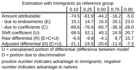
5.3.2 QR

When examining the two components ("explained and unexplained") of the immigrant-native wage gap, we …nd interesting di¤erences across the conditional wage distribution (see Table 15 for full results in Appendix). Looking at the summary of decomposition results in Table 6, we learn the raw wage gap favours natives at the bottom and immigrants at the top of the conditional wage dis-tribution. However, discrimination against immigrants does not completely die out at the top of the distribution. Further scrutiny of Table 6 shows it is primar-ily di¤erences in endowment of labour market skills of natives and immigrants, which drives changes in the wage gap across the distribution. At the bottom of the wage distribution, immigrants earn approximately 15 log percentage points because of greater labour market characteristics (E). As for those at the top of the conditional distribution, over 20 log percentage points of the wage gap is due to greater allotment of skills. Next, we turn to the shift di¤erential (U), which is the "unexplained" portion of the wage gap. It is simply the di¤erences in constants, presented as a percentage, and may owe to not controlling for more elements or factors in the model of wages. The constant of the wage equation is much greater for immigrants and this di¤erence falls across the distribution. At the 10th quantile, immigrants earn a 68.5 log percentage point gain in the constant of wages over natives in the same quantile. At the 90th percentile, the shift coe¢ cient grants immigrants 20.7 log percentage points greater earnings.

and 90th percentile, respectively).

0.10 0.25 0.50 0.75 0.90 Amount attributable: -74.5 -61.9 -44.2 -16.2 -5.0 - due to endowments (E): 15.1 14.7 16.5 20.1 23.0 - due to coefficients (C): -89.6 -76.6 -60.7 -36.3 -28.0 Shift coefficient (U): 68.5 52.1 40.1 24.9 20.7 Raw differential (R) {E+C+U}: -6.0 -9.8 -4.1 8.7 15.7 Adjusted differential (D) {C+U}: -21.1 -24.5 -20.6 -11.4 -7.3

Table 6: Summary of Decomposition Results (as %), QR Estimation with Immigrants as reference group

positive number indicates advantage to immigrants, negative number indicates advantage to natives

U = unexplained portion of differential (difference between model D = portion due to discrimination

Comparing these results with those above in the OLS decomposition, we …nd mean regression analysis covers up an important story. The OLS results show the raw di¤erential is an immigrant gain of 10.8 log percentage points and a -7.7 log percentage point loss to immigrants due to discrimination. Quantile regression analysis shows a large part of the discrimination burden is on low-ability immigrants. The raw di¤erential favouring immigrants is because of greater labour market skills and smaller di¤erences in the shift coe¢ cients of workers above the 50th percentiles.

The full quantile regression results of the decomposition indicate the di¤er-ences in skills and returns to those skills vary across the quantiles (see Table 15 in Appendix). Firstly, the endowment of years of education variable increases along the distribution. This indicates the greater ability immigrants gain more education than greater ability natives. The di¤erences in coe¢ cients on this variable illustrates a preference for natives over immigrants in providing re-turns to education. Likewise with potential experience, immigrants earn less than natives, all else equal, and this discrimination reduces across the quantiles. Yet, immigrants possess less work experience across the distribution, unlike in education. This is primarily because those individuals stay longer in education. We present summaries and full results of decompositions with natives as the reference groups (Table 16 and Table 17) and population weighted reference (Table 18 and Table 19).

5.4

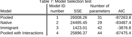
Model Speci…cation Testing

of regressors (Burnham and Anderson (2004). In least squares estimation, the AIC formula is:

AICi=nilog ^2i + 2Ki

where i indicates the model and ^2i = SSEnii. We have nis our number of

observations for modeliandKis the number of parameters, including intercept, in modeli. This measurement for the goodness-of-…t is "best" at its lowest value. Table 7 presents the AIC value for the four models for which we have OLS regression estimates. Although the native and immigrant models cannot tell us anything on their own, the native and immigrant models separately have lower AIC scores than the pooled models. This suggesting it is the "best" model(s) or way of modelling immigrant and native wages. We go on to compare the Model ID 1 and 4. These two are virtually identical with the Model 1 being minimally "better".

Model

Model ID number SSE

Number of parameters AIC Pooled 1 26008.26 31 -87263.8 Native 2 24495.45 29 -83487.4 Immigrant 3 1423.01 42 -3876.8 Pooled with Interactions 4 25896.37 44 -87475.4

Table 7: Model Selection test

The bene…t of using the Akaike criterion for model selection, as Koenker (2005) illustrates, is the natural extension for the AIC to quantile regression estimation:

AICi= log (^i) +Ki

where ^i = n 1Pni=1 1=2(yi xi^n(1=2)), which is the minimum sum of

deviations for the median regression. In Table 8, we present results for quantile estimations. We …nd the pooled model outperforms the pooled model with in-teractions. The fewer parameters in the native model suggests it is the "better" …t, however, it does not give us any indication of the marginal e¤ects for immi-grants. Therefore, along with other statistical tests, we …nd the pooled model to be the more accurate model.

Model

Model ID

number MSD

Number of parameters AIC

Pooled 1 41700.46 31 30.5

Native 2 39384.63 29 28.5

Immigrant 3 2254.18 42 41.6

Pooled with Interactions 4 41610.05 44 58.2

Table 8: Model Selection test

6

Conclusion

is essential. Any disadvantages that arise due to discrimination hold back the integration of a particular group and make it appear as though they are in-capable of economic assimilation. This can lead to undue social and political frustrations.

In the UK, immigrants have very polarised levels of education and yet, we do not observe great disparity in wages of immigrants that we do for natives. Card and Lemieux (2002) …nd that for the highly-educated, returns to educa-tion is sensitive to the supply of university graduates. Since immigraeduca-tion only a¤ects other immigrants (Manacorda et al. (2006)) and there are relatively more immigrants graduating from university than natives, we would expect greater depression on the wages of highly-educated immigrants than for natives. This may explain the minimal wage variation we observe for immigrants compared to natives. However, Martins and Pereira (2005) …nd that high-ability workers gain more from education than low-ability workers. Where high-skilled workers are more likely to gain further education (Harmon and Walker (1998)) and im-migrants have relatively higher unobserved qualities, it is ambiguous if and to what extent there are earnings disadvantages for immigrants.

Quantile regression results indicate the higher-ability individuals, or those earning a higher hourly wage conditional on all variables, gain even more from being an immigrant. In other words, immigrants are able to turn their un-observed qualities into wage growth. Those at the bottom of the conditional distribution do not earn any more than natives. Further, we …nd returns to education are far more sensitive across the immigrant than native conditional earnings distribution. This may be due to the transferability of skills. Employ-ers are not familiar with foreign education systems and do not trust or value foreign education the same as UK education.

Decomposition of immigrant and native earnings shows us the di¤erence in wages favouring immigrants is due to greater endowment of labour market characteristics. In fact, our results show that immigrants should be earning more than they do. OLS results indicate immigrants earn 10.8 log percentage points more than natives because of their characteristics. For simply being a part of the ’immigrant group’, however, there is a -7.7 log percentage point loss in wages. Much of the discrimination burden is on low-ability immigrants and increases towards zero across the conditional distribution. Below the median, discrimination reduces wages by about 22 log percentage points; whereas above the median, there is about 10 log percentage point decrease in wages due to discrimination. The di¤erence in endowments of labour market characteristics expands across the quantiles.

low-skilled workers to try. The barriers to wage growth are highly reinforced, such that the “weakest” immigrants succumb to its weight.

7

References

Albrecht, James, Anders Björklund, and Susan Vroman (2003). "Is There a Glass Ceiling In Sweden?"Journal of Labor Economics, 21, pp. 145-77.

Bauder, Harald (2006). "Origin, employment status and attitudes towards work: Immigrants in Vancouver, Canada",Work Employment Society, 20, pp. 709-29.

Blaise, Melly (2005). "Decomposition of di¤erences in distribution using quantile regression,"Labour Economics, 12(4), pp. 577-590.

Blinder, Alan (1973). “Wage Discrimination: Reduced Form and Structural Estimates”,The Journal of Human Resources, 7(4), pp. 436-55.

Borjas, George (1987). "Self-Selection and the Earnings of Immigrants,"

American Economic Review, 77(4), pp. 531-53.

Burnham, Kenneth P. and David R. Anderson (2004). "Multimodel Infer-ence: Understanding AIC and BIC in Model Selection", Sociological Methods & Research, 33(2), pp. 261-304.

Butcher, Kristin F. and John DiNardo. "The Immigrant And Native-Born Wage Distributions: Evidence From United States Censuses,"International La-bor Relations Review, 56, pp. 97-121.

Chiswick, Barry (1978). "The E¤ect of Americanization on the Earnings of Foreign-born Men",Journal of Political Economy, 86(5), pp. 897-921.

Chiswick, Barry (1980). "The Earnings of White and Coloured Male Immi-grants in Britain,"Economica, 47(185), pp. 81-87.

Chiswick, Barry and M.E Hurst (1999). "The employment, unemployment and unemployment compensation bene…ts of immigrants", Research in Employ-ment Policy, Vol. 2.

Chiswick, Barry, Anh Le, and Paul Miller (2006). "How Immigrants Fare Across the Earnings Distribution: International Analyses", Institute for the Study of Labor, IZA Discussion Paper No. 2405.

Clark, Ken and Joanne Lindley (2006). "Immigrant Labour Market Assim-ilation and Arrival E¤ects: Evidence from the UK Labour Force Survey," IZA Discussion Papers 2228, Institute for the Study of Labor (IZA).

Cotton, C. (1988). "On the Decomposition of Wage Di¤erentials", Review of Economics and Statistics, 70, pp 236-43.

Denny, K., Harmon, C., Roche, M. (1997). "The Distribution of Discrimi-nation in Immigrant Earnings: Evidence from Britain 1974-93", IFS Working Paper no. W98/3.

Dustmann, Christian, Francesca Fabbri, Ian Preston, and Jonathan Wadsworth (2003). "Labour market performance of immigrants in the UK labour market", Home O¢ ce Online Report 05/03.

"Migra-tion: an economic and social analysis", Home O¢ ce, RDS Occasional Paper No. 67.

Green, Francis, Stephen Machin, and David Wilkinson (1998). “The Mean-ing and Determinants of Skill Shortages", Oxford Bulletin of Economics and Statistics,60(2), pp. 165–88.

Harmon, C. and Ian Walker (1995). "Estimates of the economic return to schooling for the United Kingdom", American Economic Review, 85, pp.1278-86.

Koenker, Roger (2005). Quantile Regression, Cambridge University Press. Lee, Sokbae (2007). "Endogeneity in quantile regression models: A control function approach",Journal of Econometrics, 141, pp. 1131-58.

Machado, José A. F. and José Mata (2000). "Counterfactual decomposition of changes in wage distributions using quantile regression", Journal of Applied Econometrics 20(4), pp. 445-65.

Machado, José A. F. and José Mata (2001). "Earning functions in Portugal: evidence from quantile regressions",Empirical Economics, 26(1), pp. 115–134. Oaxaca, Ronald (1973). “Male-Female Wage Di¤erentials in Urban Labor Market",International Economic Review,14(3), pp. 693-709.

Oaxaca, Ronald and Michael Ransom (1999). "Identi…cation in Detailed Wage Decompositions", The Review of Economics and Statistics, 81(1), pp. 154-57.

Ottaviano, G. and Peri, G. (2005). “Rethinking the Gains From Immigra-tion: Theory and Evidence from The U.S.", NBER Working Paper No. 11672. Wooldridge, Je¤rey (2002). Econometric Analysis of Cross Section and Panel Data, MIT Press.

8

Appendix A

LOG REAL HOURLY WAGE- The LFS does not ask income questions to the self-employed. LFS asks all persons 16-69, and those over 70 whom are employed. ‘Gross weekly pay in main job’(GRSSWK) is asked each quarter, but only to individuals in their 5th wave. From 1997 onwards, the question was asked in the 1st wave as well. For those answering both, we checked for any signi…cant disparities or changes from the 1st to 5th wave; there were none. If GRSSWK is greater than £ 3,500, or GRSSWK is greater than £ 1,000 and the respondent is a manual worker, then the LFS does not give an income weight. Non-response to this question is also be zero-weighted. LFS Users Guide indicates standard …lters used to calculate average gross weekly earnings are GRSSWK>0. To generate hourly pay, we also …lter on ‘usual hours excluding overtime’, USUHR>0. To produce real wages, we use the U.K Retail Price Index to in‡ate wages based on 2005Q4 prices. We then generate logarithm of the gross real hourly wage.

the UK. We subtract DOBY from CAMEYR to derive AGEAIM. For the native-born, this variable takes on a value of zero.

EDYRS (Years of education)- is equal to the reported education leaving age (EDAGE) minus 5 (to account for the age of starting school).

ENG (Native English-speaker)- is a dummy variable taking a value of 1 if the respondent reports a "typical" English-speaking country of origin. These countries are: England, Wales, Scotland, Ireland, United States, Canada, Australia, New Zealand, South Africa, and any of the Caribbean islands.

EXP (Potential work experience)- is potential labour market experience derived from the respondents’ age (AGE) minus leaving age from education (EDAGE) for individuals who responded to EDAGE. If an individual answered (s)he ‘never had any education’, we use age minus 15. This is because there is a legal working age and leaving age from education.

FTPT (Full-time, Part-time)- We construct this dummy variable from reported usual hours in a week excluding overtime (USUHR). The variable takes a value of 1 if the respondent works less than 30 hours, and a value of zero otherwise.

HEAL(Health status)- is a dummy taking a value of 1 if the respondent answers ’yes’to the question of any health problems lasting more than one year (HEALYR), 0 if answers ’no’.

INDUS (Industries)- is only reported by respondents in employment and not tied to company sponsored college. There are ten categories: (1) Agricul-ture and …shing, (2) Energy and water, (3) Manufacturing, (4) Construction, (5) Distribution, hotels, and restaurants, (6) Transport and communication, (7) Banking, …nance, and insurance, (8) Public administration, education, and health, (9) Other services.

MARC (Married, Cohabiting)- we use the variable ‘marital status’, MARSTT, and ’living together as a couple’, LIVTOG. We move all the re-sponses of ‘does not apply’or ‘no answer’to missing. Our variable takes a value of 1 if the response is ‘married, living with husband or wife’or a ’yes’response to LIVTOG, and 0 otherwise.

NONW (Nonwhite)- There are several ethnicity variables over time (ETH01, ETHCEN15, ETHCEN6), which we recoded for consistency: (1) White, (2) Mixed, (3) Asian or Asian British, (4) Black or Black British, (5) Chinese, (6) Other. We then give a value of 0 to responses of white and 1 otherwise.

REGOB (Region of Birth)- There are several country of origin variables over time (CRY, CRY01, CRYOX, CRYO), which we recoded for consistency. Many country cells had small numbers of respondents, thus we grouped the countries into major regions: (1) Ireland, (2) Caribbean & West Indies, (3) China/HK, (4) Europe, (5) India, (6) Pakistan/Bangladesh, (7) Old Common-wealth & US, (8) Rest of the World.

URESMC (Region of inhabitance)- We create dummies to the response of ‘region of usual residence’, URESMC. We create one response of inner and outer London, as well as Strathclyde and Rest of Scotland. We drop Northern Ireland.

arrival (CAMEYR) into the UK from the survey year. For the native-born, this variable is the derived variable (AGE) that comes from subtracting the survey year from the year of birth (DOBY).

FORx (Potential overseas work experience)- if age at immigration (AGEAIM) is greater than leaving age of education (EDAGE), then the re-spondent has some potential work experience before entering the UK and this variable takes a value of 1.

9

Appendix B

9.1

Tables

OLS

Dependent variable: Log real hourly wage 0.10 0.25 0.50 0.75 0.90

Constant 0.914** 0.539** 0.704** 0.884** 1.095** 1.288**

(97.65) (27.73) (64.98) (73.43) (90.34) (80.64)

Potential Experience 0.055** 0.049** 0.052** 0.055** 0.058** 0.059**

(128.43) (84.88) (109.79) (110.18) (163.76) (68.97)

Potential Experience^2 -0.001** -0.001** -0.001** -0.001** -0.001** -0.001**

(-108.96) (-79.74) (-92.05) (-96.74) (-118.42) (-52.96)

Years of Education 0.079** 0.074** 0.078** 0.08** 0.081** 0.084**

(142.24) (77.71) (124.60) (112.14) (89.19) (68.06)

Nonwhite -0.144** -0.156** -0.158** -0.137** -0.109** -0.105**

(-16.52) (-9.14) (-13.70) (-12.02) (-9.86) (-8.71)

Married & cohab 0.084** 0.094** 0.088** 0.083** 0.077** 0.078**

(29.77) (19.05) (23.11) (32.80) (31.78) (16.71)

NonEnglish Mother tongue -0.131** -0.16** -0.141** -0.122** -0.117** -0.122**

(-10.37) (-8.03) (-8.00) (-7.62) (-6.89) (-4.67)

Immigrant dummy 0.042** 0.001 0.029 0.030** 0.052** 0.091** (4.11) (0.10) (1.55) (3.08) (3.35) (4.93)

Industries (omit Construction)

Agriculture & Fishing -0.336** -0.301** -0.322** -0.331** -0.332** -0.326**

(-27.71) (-21.21) (-36.52) (-23.88) (-19.68) (-21.36)

Energy & Water 0.158** 0.181** 0.156** 0.141** 0.163** 0.161**

(18.40) (14.00) (16.95) (19.11) (22.95) (14.19)

Manufacturing 0.045** 0.026 0.041** 0.024 0.053** 0.074**

(3.98) (1.17) (2.79) (1.91) (4.31) (4.70)

Distribution, Hotels & Restaurants -0.193** -0.223** -0.214** -0.203** -0.173** -0.131**

(-44.77) (-33.81) (-54.10) (-45.87) (-33.18) (-15.13)

Transport & Communication -0.014** -0.003 -0.01* -0.018** -0.012* 0.01

(-2.87) (-0.35) (-2.27) (-4.43) (-2.53) (1.11)

Banking, Finance & Insurance etc 0.123** 0.022** 0.08** 0.118** 0.167** 0.216**

(28.86) (2.79) (-14.42) (23.87) (31.67) (34.56)

Public admin, Educ & Health -0.007** 0.008 0.023** 0.007* -0.012** -0.045**

(-1.61) (-1.41) (5.42) (2.43) (-3.61) (-7.89)

Other Services -0.094** -0.104** -0.106** -0.103** -0.087** -0.065**

(-22.53) (-17.86) (-23.61) (-21.93) (-22.49) (-10.83)

Regions (omit South East)

Tyne & Wear -0.175** -0.14** -0.156** -0.166** -0.185** -0.202**

(-18.32) (-8.38) (-17.79) (-18.47) (-18.72) (-12.36)

Rest of Northern Region -0.159** -0.148** -0.156** -0.148** -0.156** -0.173**

(-21.92) (-11.30) (-17.01) (-22.57) (-19.37) (-14.05)

South Yorkshire -0.184** -0.158** -0.147** -0.163** -0.188** -0.234**

(-20.59) (-10.00) (-12.52) (-19.53) (-19.71) (-19.23)

West Yorkshire -0.158** -0.109** -0.134** -0.155** -0.174** -0.192**

(-22.62) (-13.66) (-19.50) (-18.94) (-23.29) (-16.38)

Rest of Yorkshire & Humberside -0.175** -0.173** -0.161** -0.16** -0.172** -0.185**

(-22.26) (-17.16) (-17.95) (-17.88) (-27.78) (-17.35)

East Midlands -0.145** -0.095** -0.124** -0.143** -0.155** -0.168**

(-27.07) (-12.38) (-16.25) (-22.78) (-22.62) (-15.64)

East Anglia -0.13** -0.087** -0.108** -0.126** -0.144** -0.155**

(-18.69) (-7.23) (-19.45) (-19.25) (-19.89) (-14.88)

Inner & Outer London 0.07** 0.077** 0.072** 0.075** 0.073** 0.078**

(13.52) (8.44) (14.09) (11.50) (10.50) (10.45)

South West -0.149** -0.123** -0.131** -0.14** -0.161** -0.172**

(-29.35) (-17.36) (-20.05) (-22.01) (-24.92) (-26.32)

West Midlands (Metro) -0.146** -0.107** -0.115** -0.139** -0.166** -0.184**

(-21.42) (-11.16) (-12.02) (-20.09) (-23.33) (-22.17)

Rest of West Midlands -0.149** -0.101** -0.132** -0.15** -0.167** -0.196**

(-24.20) (-18.77) (-22.02) (-20.81) (-22.94) (-19.45)

Greater Manchester -0.144** -0.119** -0.124** -0.139** -0.15** -0.184**

(-20.73) (-11.28) (-14.30) (-18.94) (-17.53) (-14.72)

Merseyside -0.169** -0.125** -0.132** -0.156** -0.183** -0.206**

(-16.84) (-6.89)* (-14.77) (-16.55) (-20.22) (-21.91)

Rest of North West -0.141** -0.127** -0.127** -0.119** -0.138** -0.15**

(-20.67) (-15.87) (-21.75) (-20.78) (-16.22) (-18.14)

Wales -0.198** -0.173** -0.182** -0.194** -0.2** -0.214**

(-29.98) (-14.85) (-25.58) (-23.00) (-24.41) (-18.82)

Strathclyde & Rest of Scotland -0.147** -0.123** -0.135** -0.146** -0.153** -0.163**

(-30.25) (-19.51) (-25.93) (-28.26) (-19.81) (-14.01)

Observations 126,877 126,877

R-squared 0.33 0.17 0.20 0.22 0.22 0.21

Table 9: OLS & Quantile Regression Results for Pooled Model Quantiles

Dependent variable: Log real hourly wage .10 .25 .50 .75 .90

Constant 0.109** -0.379** -0.027** 0.195** 0.381** 0.515**

(2.89) (-5.41) (-0.59) (3.94) (9.89) (7.40)

Year trend 0.008** 0.01** 0.008** 0.007** 0.007** 0.008**

(21.92) (13.67) (15.54) (13.20) (16.61) (11.14)

Personal variables

Potential Experience 0.055** 0.049** 0.052** 0.055** 0.058** 0.059**

(129.02) (73.09) (102.49) (117.37) (143.60) (78.26)

Potential Experience^2 -0.001** -0.001** -0.001** -0.001** -0.001** -0.001**

(-109.76) (-60.58) (-83.49) (-87.23) (-113.71) (-61.10)

Years of Education 0.077** 0.073** 0.077** 0.079** 0.08** 0.082**

(139.96) (100.18) (121.72) (111.13) (102.87) (86.19)

Nonwhite -0.149** -0.162** -0.164** -0.14** -0.114** -0.112**

(-17.16) (-10.25) (-18.68) (-16.46) (-12.55) (-8.07)

Married & cohab 0.078** 0.088** 0.085** 0.077** 0.070** 0.073**

(27.20) (21.57) (29.82) (22.32) (20.52) (17.59)

NonEnglish Mother tongue -0.133** -0.185** -0.139** -0.13** -0.122** -0.133**

(-10.30) (-7.38) (-7.76) (-12.23) (-5.73) (-7.27)

Foreign variables (omitted 1993)

Immigrant dummy 0.073 0.015 0.047 0.058 0.042 0.007

(1.17) (0.19) (0.50) (1.71) (0.52) (0.05)

Foreign*1994 0.045 0.03 -0.041 0.004 0.155 0.299*

(0.57) (0.23) (-0.33) (0.07) (1.94) (1.99)

Foreign*1995 -0.095 -0.051 -0.038 -0.046 -0.149 0.022

(-1.17) (-0.55) (-0.29) (-0.64) (-1.41) (0.13)

Foreign*1996 0.001 0.033 0.061 0.024 0.001 0.065

(0.01) (0.28) (0.62) (0.42) (0.01) (0.52)

Foreign*1997 -0.073 -0.042 -0.058 -0.057 -0.049 0.035

(-1.11) (-0.51) (-0.60) (-1.24) (-0.55) (0.22)

Foreign*1998 -0.074 -0.045 -0.075 -0.089* -0.024 0.057

(-1.13) (-0.49) (-0.70) (-2.13) (-0.27) (0.38)

Foreign*1999 -0.042 -0.015 -0.056 -0.04 0.008 0.079

(-0.64) (-0.17) (-0.57) (-1.22) (0.10) (0.53)

Foreign*2000 -0.072 -0.072 -0.021 -0.041 -0.013 0.047

(-1.11) (-0.75) (-0.19) (-1.03) (-0.16) (0.33)

Foreign*2001 0.046 0.051 0.039 0.059 0.09 0.241

(0.69) (0.67) (0.37) (1.47) (1.12) (1.80)

Foreign*2002 0.012 0.018 -0.005 0.033 0.076 0.153

(0.18) (0.25) (-0.05) (0.68) (0.88) (1.09)

Foreign*2003 -0.034 0.009 -0.005 -0.033 -0.007 0.086

(-0.52) (0.11) (-0.05) (-0.90) (-0.08) (0.62)

Foreign*2004 -0.073 -0.056 -0.076 -0.062 -0.031 0.069

(-1.11) (-0.66) (-0.82) (-1.64) (-0.35) (0.47)

Foreign*2005 -0.035 0.016 -0.028 -0.025 0.014 0.072

(-0.54) (0.19) (-0.27) (-0.51) (0.16) (0.51)

Industry variables (omitted Construction)

Agriculture & Fishing -0.335** -0.30** -0.314** -0.332** -0.337** -0.333**

(-27.66) (15.20) (26.37) (24.57) (33.95) (16.32)

Energy & Water 0.161** 0.182** 0.16** 0.141** 0.164** 0.167**

(18.75) (19.89) (15.46) (18.75) (15.36) (12.70)

Manufacturing 0.089** 0.082** 0.083** 0.064** 0.092** 0.12**

(7.69) (3.26) (4.66) (6.32) (7.36) (6.69)

Distribution, Hotels & Restaurants -0.196** -0.226** -0.215** -0.207** -0.18** -0.135**

(-45.53) (30.93) (41.89) (54.71) (32.33) (22.65)

Transport & Communication -0.018** -0.004 -0.007 -0.018** -0.018** 0.002

(-3.59) (-0.46) (-1.10) (3.83) (3.13) (-0.25)

Banking, Finance & Insurance etc 0.12** 0.02** 0.079** 0.118** 0.165** 0.208**

(28.16) (2.65) (11.42) (32.72) (36.97) (28.45)

Public admin, Educ & Health -0.007 0.006 0.021** 0.008** -0.012** -0.046**

(-1.82) (1.03) (4.28) (1.63) (3.19) (10.59)

Other Services -0.098** -0.109** -0.107** -0.105** -0.091** -0.07**

(-23.55) (16.97) (19.53) (20.89) (18.65) (11.15)

Regional variables (omitted South East)

Tyne & Wear -0.176** -0.134** -0.16** -0.174** -0.186** -0.211**

(-18.51) (6.82) (12.66) (17.22) (30.54) (16.93)

Rest of Northern Region -0.159** -0.145** -0.158** -0.149** -0.157** -0.173**

(-21.94) (19.12) (22.01) (13.02) (20.85) (17.03)

South Yorkshire -0.185** -0.145** -0.148** -0.168** -0.193** -0.237**

(-20.74) (12.28) (14.59) (21.87) (22.60) (19.37)

West Yorkshire -0.16** -0.113** -0.137** -0.158** -0.177** -0.194**

(-22.91) (10.73) (14.40) (25.32) (26.90) (18.52)

Rest of Yorkshire & Humberside -0.176** -0.169** -0.169** -0.162** -0.174** -0.186**

OLS Quantile Regression

(-22.43) (15.72) (16.72) (21.74) (22.70) (12.48)

East Midlands -0.146** -0.097** -0.127** -0.144** -0.159** -0.171**

(-27.32) (12.68) (23.22) (27.16) (29.44) (20.93)

East Anglia -0.129** -0.087** -0.107** -0.13** -0.142** -0.147**

(-18.62) (7.54) (12.29) (18.95) (23.40) (23.21)

Inner & Outer London 0.073** 0.08** 0.074** 0.075** 0.072** 0.084**

(-14.17) (8.63) (11.37) (11.47) (11.86) (11.64)

South West -0.15** -0.124** -0.135** -0.14** -0.162** -0.17**

(-29.62) (16.35) (22.44) (22.84) (28.59) (29.68)

West Midlands (Metro) -0.145** -0.101** -0.114** -0.141** -0.164** -0.182**

(-21.33) (8.97) (16.33) (19.91) (21.79) (21.45)

Rest of West Midlands -0.149** -0.098** -0.134** -0.151** -0.166** -0.194**

(-24.30) (10.85) (22.48) (24.99) (26.45) (26.50)

Greater Manchester -0.143** -0.118** -0.126** -0.137** -0.153** -0.187**

(-20.66) (13.21) (22.09) (24.73) (25.54) (22.28)

Merseyside -0.167** -0.123** -0.131** -0.155** -0.182** -0.206**

(-16.65) (8.23) (12.26) (15.62) (16.05) (17.92)

Rest of North West -0.14** -0.124** -0.125** -0.119** -0.137** -0.15**

(-20.51) (10.50) (18.47) (15.46) (18.40) (21.66)

Wales -0.199** -0.167** -0.186** -0.195** -0.202** -0.213**

(-30.09) (21.24) (26.02) (31.10) (26.27) (30.27)

Strathclyde & Rest of Scotland -0.149** -0.12** -0.139** -0.146** -0.154** -0.164**

(-30.56) (14.58) (20.74) (25.96) (39.95) (23.76)

Observation 126,877 126,877

Pseudo R-squared 0.33 0.17 0.20 0.22 0.22 0.21