Interference robust spatial multiplexing

(1)

1

Faculty of Electrical Engineering,

Mathematics & Computer Science

Interference Robust

Spatial Multiplexing

Jippe R. Rossen M.Sc. Thesis June 19, 2018

Supervisors: Dr. ir. A.B.J. KOKKELER

Dr. ing. E.A.M. KLUMPERINK

Dr. ing. D.M. ZIENER

(2)

(3)

Jippe Rossen Master Thesis

Abstract

This project focuses on the practical application of techniques regarding spatial multiplexing. Spatial multiplexing is implemented by estimating the channel matrix using a least squares ap-proximation. The obtained channel matrix is decomposed using a singular value decomposition. The resulting singular values and singular vectors for various scenarios are related back to the principles of spatial multiplexing.

A simulation environment is created to make the techniques more insightful and to provide a baseline performance on what to expect from practical scenarios. Using standard building materials and basic RF equipment, a setup is constructed to do practical experiments. Experi-ments are carried out to characterize the behavior of the transceiver system in both a controlled environment as well as in practical scenario’s.

(4)

(5)

Acknowledgements

I would like to thank my supervisors Andr´e, Eric and Massoud for their guidance, their insights and the useful discussions I have had with all of them. I am also especially appreciative for their patience and allowing me the time to do countless other activities in parallel to my graduation project.

I would also like to express my thanks to Henk de Vries for providing various pieces of lab equipment and his advise on how to get the best lab results.

I am grateful for the support I received from Robert Vogt-Ardatjew. His knowledge on the specifics of anechoic chambers has proven most helpful and has contributed to this research a lot.

I would like to thank all people of the research group of Computer Architecture for Embed-ded Systems for the great time I have had whilst working on my graduation project. A special thanks I would like to give to Hendrik Folmer and Robert de Groote for putting up with me in an office. It has provided a very nice environment for me to work in and I had great time with you guys.

(6)

(7)

Introduction

With the progress in processing power in digital communication systems, many new techniques to increase performance have been invented. There remain, however, a few complications in such systems. Multi path fading causes systems to introduce self interference when communication signals in the form of electromagnetic signals are reflected by objects along the transmission path. These reflections cause delayed instances of the original signal on the receiver of the communication line. These delayed instances add to other interference signals and deteriorate the Signal to Noise Ratio (SNR).

Also, as the number of communication systems increase, the allocated frequencies in the elec-tromagnetic spectrum become more crowded. Especially in dense urban areas, local wireless networks interfere with one another to such an extent that a substantial decrease in performance is perceived.

By employing Direction of Arrival (DOA) estimation techniques it is possible to determine the angle of incidence of incoming signals. The receiver can be tuned to only receive signals from a particular direction, which effectively cancels undesired signals from other directions, which is called beamforming. There has been a vast amount of research on this topic ([1],[2]). When the transmitter is also equipped with an array of antennas, also the transmitted beamfront can be steered. By using superposition, multiple signals can be transmitted in multiple directions. When these techniques are used at the same time, many different combinations of transmit and receive angles are possible, which will result in many different channels.

When the receiver antenna array has M elements and the transmitter array has N anten-nas, each of the antenna combinations between transmitter and receiver has its own transfer characteristics. A channel matrix can be constructed which consists of M by N elements, which characterizes the transfer between each individual antenna pair. One of the aspects of this project is to determine and describe how this matrix corresponds to the spatial transmission paths and how these are affected by neighboring systems. Evaluations will be performed on how spatial multiplexing can be applied in a robust way to limit the effects of interference from these neighboring systems. Simulations will be performed in combination with real physical evaluations to validate proposed techniques.

Concluding, the research goals of this project are:

1. Explore existing literature on channel estimation, Singular Value Decomposition and/or Principal Component Analysis in the context of spatial multiplexing.

(10)

CHAPTER 1. INTRODUCTION

3. Find for 4x4 Multiple Input Multiple Output (MIMO) channels the optimal spatial trans-mission paths.

(11)

Chapter 2

Transmission Techniques and

Characteristics

2.1 Global outline

To address the research goals, a simple use case will be introduced to indicate the topics on which this project focuses. This arbitrary case will then be utilized to elaborate on more in-depth concepts of the tasks at hand. First this will be explored using Matlab simulations, after which it will be tested in real scenarios using actual hardware.

Figure 2.1 shows an arbitrary environment in which a communication system is employed of two antennas (A1, A2), both capable of transmitting and receiving. For simplicity and clearity,

suppose that A1 is only used for transmission and A2 is only used for receiving. As both A1

and A2 have only a single transmitter and a single receiver, this system can be considered as a

Single Input Single Output (SISO) system.

Figure 2.1: Communication system in an arbitrary environment.

As soon as A1 starts transmitting data, Electromagnetic (EM)-waves start propagating

(12)

CHAPTER 2. TRANSMISSION TECHNIQUES AND CHARACTERISTICS

(a) 0 degrees (b) 30 degrees (c) 60 degrees

Figure 2.2: Directional sensitivity for specific steering angles of an antenna array.

occupies the same frequency band, the desired signal is lost.

In figure 2.1 the transmitter and the receiver are single antennas. If now these antennas are replaced by arrays, the linear phased-array setup of figure 2.3 is created. Both A1 and A2

are now equipped with four antennas each (nr, nt= 4), making it a MIMO system. By adding delays (phase shifts) to the received signals and summing the results, the antenna can be made directional. Figures 2.2a through figure 2.2c show the resulting gain of the array against the Angle of Incidence (AoI) when the receiver array is set for a steering angle of 0°, 30°and 60°. This makes beamforming quite effective in the suppression of unwanted signals from angles of no interest. Especially the concept of null steering can be very effective to suppress known interferers[3]. In the end, however, all it does is raising the SNR of a transmission link.

Shannon’s theorem for link capacity (equation 2.1) dictates that the increase of SNR can be used to improve the channel’s capacity[4]. Because of the logarithmic nature of this equation, doubling the SNR will provide only a very limited increase in the data rate. By applying spatial multiplexing this logarithmic relation can be avoided as the spectral efficiency can be increased linearly with the number of paths.

C=B·log2(1 +

S

N) (2.1)

2.2 Steering vectors

A linear phased array can be made sensitive to a certain angle by employing a so called steering vector. This vector, which has the same dimension as the number of antennas in the array, con-tains a phase rotation and a gain for each separate antenna. These phase rotations cause the received signals on the antennas to be in the same phase resulting in constructive interference for the angle of the steering vector and destructive interference for other angles.

(13)

[image:13.595.139.457.80.281.2]

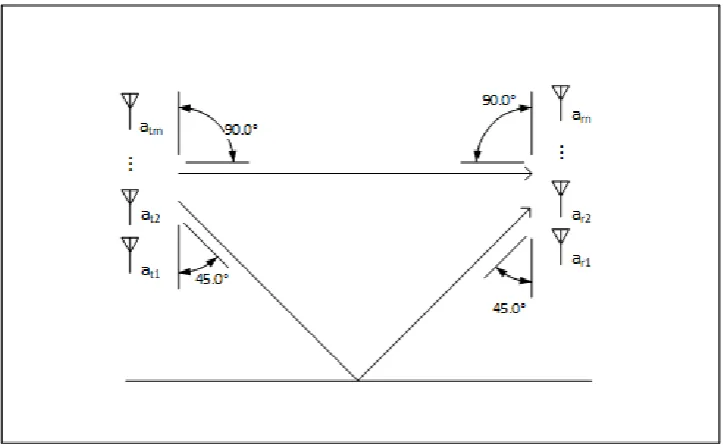
Figure 2.3: Communication system with linear phased array antennas on both the receiver as the transmitter side.

2.3 Multipaths & spatial multiplexing

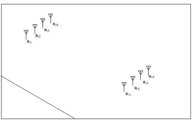
In figure 2.4, the simple model of figure 2.3 is extended with the spatial transmission paths possible in this environment. The direct path between both arrays is still present. However, also a secondary path is shown which originates by a reflection on a wall. The first signal has an AoI of 0°, where the second has an AoI of -45°. Assuming that it is possible to mathematically separate and isolate these signals, it should be possible to send two different streams of data over the two individual channels. The technique of transmitting multiple streams of the same frequency in the same space at the same time is known as spatial multiplexing.

There are some complications about using spatial multiplexing. When signals are broadcast at the same time at the same frequency, they start interfering with one another. The receiver array can be made sensitive to a certain direction, but will generally not be able to completely cancel signals from other angles. This interference has a direct impact on the SNR. Another issue is that the sensitivity of the array to a certain direction is limited by the number of an-tennas in the array. For the array to be able to cancel signals from unwanted directions they should have a large enough angular separation to prevent them from interfering too much with one another.

2.4 Channel characteristics

To identify suitable transmission paths, the channel has to be characterized. A model has to be made that describes how the transmitted signals of each antenna are subjected to alterations in phase and gain. This is done by determining the channel transmission matrix H, which is also known as the Channel State Information (CSI).

2.4.1 The channel matrix

(14)

[image:14.595.117.479.84.308.2]

Figure 2.4: Communication system with a direct path and a reflection path.

the gain (loss) and the phase of each possible transmit and receive antenna pair. The received signal can then be described by:

y=Hx+w (2.2)

In which x is a vector containing the transmitted signal by at1..atm and y is a vector containing the signals received by antennasar1..arn (which are defined in figure 2.4). His a m by n matrix containing the transfer function of every possible antenna pair in the system. The values of H are complex, as they need to contain both the amplitude and the phase relation. In this equationwdenotes the noise that is present in the system. It is assumed that the noise is white Gaussian in nature.

2.4.2 Estimation of a channel

So far it was assumed that H was known to both receiver and transmitter. In any realistic scenario this is not the case, thus it has to be estimated. To do this a training sequence is required. The training sequence is known to both the receiver and the transmitter and is used to determine the transfer function between all possible combination pairs of transmitter and receiver antennas. A lot of research has been done on the topic of optimal training sequences for specific systems and environments [5]. As the proposed setup is a stand-alone communication system in an arbitrary environment, the transfer function and noise distributions are unknown. Therefore a least squares estimation is best suited to find the H matrix[6, chapter 3], see equation 2.3.

HLS−estimate=YP∗(PP∗)−1 (2.3)

(15)

Figure 2.5: Graphic reepresentation of decomposing the channel matrix into multiple SISO channels. The and V∗ matrix maps the signals to eigenmodes and the U matrix maps them back to the original coordinate frame. [10]

sequence is multiplied by a factor q.

2.4.3 Multiplexing capability

The effectiveness of spatial multiplexing is strongly dependent on the surroundings. It will be assumed that the channel matrix H is time-invariant1. In this section also the assumption is taken that the channel matrix is known to both transmitter and receiver. To understand how the characteristics of Hdetermine the spatial multiplexing capabilities of a wireless channel, a closer look at the capacity of the channel is taken.

In equation 2.2 the relation between a transmitted signal, the received signal and the trans-mission matrix Hwas introduced. Linear algebra shows that every matrix can be decomposed into three other matrices, a rotation matrix, a scaling matrix and another rotation matrix, which is called a Singular Value Decomposition (SVD)[7, Chapter 3]. This operation can be interpreted as two coordinate transformations and a simple scaling operation. The coordinate transformations effectively map the MIMO channel into multiple parallel SISO channels, which can be called eigenmodes. For each of these channels Shannon’s link capacity theorem holds. This also shows how spatial multiplexing can improve the link capacity. Equation 2.4 shows this decomposition mathematically and figure 2.5 shows how the result of this operation can be interpreted as multiple SISO channels.[8, Chapter 7][9]

H=UΛV∗ (2.4)

In equation 2.4,UandV∗ are both unitary matrices (M−1=M∗) giving them the property that MM∗ =M∗M=I, with I being the identity matrix. The columns of a unitary matrix form an orthonormal set. The vectors of theUmatrix are also known as the left singular vectors and the ones from theV∗ matrix the right singular vectors.

Figure 2.5 shows that the vectors of these matrices are used for coordinate transformations at both the receiver as the transmitter. These transformations map the signals onto the

eigen-1

(16)

modes and map them back to the original coordinate frame. As the eigenmodes are in this case spatial paths, the vectors of these matrices act as steering vectors for the system.

Λis a rectangular matrix with on its diagonal the real-valued singular values (λ1 ≥λ2≥λn)

of the matrixH and all off-diagonal elements are zero (see 2.5). The dimensions of Λ are de-pendent on the number of antennas in both the transmitting (nt) as the receiving array (nr). Λ may therefore not be square.

Λ=     

λ1 0 . . . 0

0 λ2 . . . 0

..

. ... . .. ... 0 0 . . . λn

     (2.5)

These singular values indicate the suitability of an environment for spatial multiplexing. The singular values each correspond to an eigenmode and are ordered from strongest to weak-est. For a perfect scenario all these singular values would have the same value. In that case the power could be distributed equally giving the maximum link capacity. This scenario actually only exists when the eigenmodes are guided from transmitter to receiver through cables, which isolates each eigenmode completely from one another.

For a wireless system the signals do interfere with one another causing the singular values to drop off. The lower a singular value is, the weaker the corresponding eigenmode will be. The singular values should be assessed simultaneously with the SNR to see whether it makes sense to allocate power to a specific eigenmode at the SNR of that eigenmode. This allocation of power is generally done using waterfilling techniques. During waterfilling, power is allocated to the eigenmodes to achieve optimal link capacity. As this depends on both the SNR and the singular values, it is difficult to give a general statement on when an eigenmode is suitable for spatial multiplexing.

The number of singular values and eigenmodes are limited by the number of antennas in both the transmission array as the receiving array: n = min(nt, nr). This implies that the maximum number of eigenmodes available is equal to the smallest number of antennas in either of the arrays.

2.4.4 Condition number

To determine how many paths are suited for spatial multiplexing, some sort of measure is required. The concept of the condition number can be used for this purpose[11, p100]. The condition number is defined by:

CN = maxλn

minλn

(2.6)

The condition number only gives a measure on the weakest eigenmode with respect to the strongest eigenmode. The waterfilling techniques could opt to only use the strongest eigenmode or the two strongest eigenmodes. In that sense the condition number is not that useful. It does however give a good indication on how well the channel matrix is conditioned.

(17)

always 1 and the last being always equal to the condition number. These condition ratios will quickly give an indication of the suitability of each eigenmode for spatial multiplexing.

2.5 Synchronization

Up until now it was assumed that only a phase shift was present in the communication line be-tween transmitter and receiver. The fact that the receiver and transmitter are not synchronized does introduce some complications. During sampling the signals are subject to an arbitrary off-set in samples. The least squares estimation presented above requires the pilot signal’s samples to be aligned with the received signals so this has to be dealt with.

The offset in samples can be determined by performing a cross correlation between the training signals and the received signals[12]. For every transceiver channel pair (for example

at1−ar1), the cross correlation operation results in a vector of correlation values between the

transmitted signals and the received signals. By summing the magnitudes of the correlations of the individual channels, a vector of combined correlations can be found for the offset between the received signals and the pilot signals. The maximum combined correlation is the assumed offset and is used to synchronize the two signal sets2.

2.6 Direction of arrival

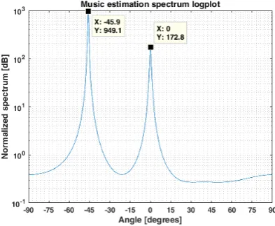
Although it is not necessary for spatial multiplexing, the DOA algorithm Multiple Signal Clas-sification (MUSIC)[13] can be used to visualize the relation between the angle of incidence and the received power more distinctly. MUSIC works by using the system’s noise subspace to find the DOA of the received signals. The subspaces are found by calculating the eigenvalues (D) and eigenvectors (V) of the co-variance matrix of the received signals. This results in a num-ber of eigenvectors equal to the numnum-ber of receive antennas. Each of these eigenvectors can be considered a subspace. By choosing how many of these belong to the noise subspace, the number of peaks found by the music algorithm can be controlled. If the noise subspace uses all eigenvectors but one, only a single peak will be detected (the noise subspace is in that case of dimension n-1 and the signal subspace has only a single dimension).

Leta(φ,n) be a steering vector consisting of n elements, in which n is the number of antennas in the receiver. This research focuses on the use of linear phased arrays therefore a(φ,n) will be defined as is shown in equation 2.7.

a(φ,n) =

        

e−i·ω·fcarrierc ·∆·0·sin(φ)

.. .

e−i·ω·fcarrierc ·∆·(n−1)·sin(φ)

         (2.7)

2_{The presented operation works only on a communication system where the number of transmit antennas is}

(18)

[image:18.595.194.391.91.253.2]

Figure 2.6: Direction of Arrival results by employing the MUSIC algorithm.

The noise subspace, En, will be spanned by selecting the eigenvectors that correspond to the lowest n eigenvalues (in which n depends on the desired dimension of the signal subspace). The product of the steering vector with the noise subspace should be high everywhere except for the angles in which a signal resides. By finding the peaks resulting from equation 2.8, the DOA’s can be obtained.

P= 1

a(φ)·En·En∗_·_a₍_φ₎ (2.8) Figure 2.6 shows the results of MUSIC graphically for a system with two incoming wave-fronts, one from 0° and one from -45°(which is the situation of figure 2.4). This plot has been made by selecting two eigenvectors for the noise subspace and that the MUSIC algorithm indeed produces peaks at 0°and -45°.

2.7 Interference suppression and reduction

In section 2.4.3 it was explained that spatial multiplexing operates by applying a singular value decomposition on the channel matrix to determine a set of singular vectors. These vectors are created by an estimation of the channel matrix. When estimating the channel matrix, in-terference may be present in the system. The inin-terference introduces significant errors as the estimation of the channel will find a correlation between received signals and transmitted pilot signals which are caused by the interference and not by the actual transfer between transmitter and receiver. The channel estimation itself may also become impossible when the system cannot distinguish the training sequence because of the interference.

(19)

can be used as a transformation matrix on the received samples (Y) to create Yfiltered (See

equation 2.9). In this operation the matrix F∗ will act as a spatial filter, because the subspace that holds the interference was removed from this matrix3.

Yfiltered=F∗Y (2.9)

Because F∗ is a 3x4 matrix, the dimension ofYfiltered will be reduced by one. This results

in the channel estimation producing a 3x4 matrix as the system now transmits four channels and the estimation is performed by only three receiver signals. The eigenvectors that are used inF∗ also contain phase rotations, which cause the received signalsYfilteredto be in a different

coordinate frame. The left singular vectors of the singular value decomposition now no longer only relate to the phase shifts required for the steering vectors, but also the ones for the filter. This can be resolved by left-multiplying Yfiltered with F, which results in the operation as

shown in 2.10.

Yfiltered=FF∗Y (2.10)

Since the eigenvectors of V are orthonormal, the column vectors of F are also orthonor-mal. F is thus an n by n-1 matrix with orthonormal columns. For such matrices holds that FF∗Y=projWYfor all YinCn, where W is the column space of the matrix F[15, p42]. This proves that equation 2.10 effectively projects the signals of Y onto a n-1 dimensional space (which does not contain the subspace that belongs to the interference) and back to the original coordinate frame that once again holds n dimensions.

This approach does have a downside. The modified transformation matrix was determined solely on the presence of interfering signals (the system’s own transmitters were mute). This means that the subspace vectors that are conserved are completely unrelated to the channel between transmitter and receiver. It may thus very well be possible that there are nulls present for angles that are in fact necessary for spatial multiplexing in that situation. The impact of this shortcoming reduces as the number of antennas in the array increases. The remaining sub-space vectors are based on White Gaussian Noise (WGN) and should thus spread themselves out over the angular spectrum, whilst all having a null at the angle of the interferer. With more antennas in the array, there are more degrees of freedom available for the null steering giving a more balanced result.

The spatial multiplexing algorithms will now useYfilteredinstead ofY. Every signal coming

from the angle of the interferer will be suppressed by the spatial filter. The left singular vectors will thus be impervious to signals from this angle and their angular sensitivity plots should therefore show a null at this angle.

In this research the data flows solely from transmitter to receiver, in other words, the arrays do not switch roles. In a normal communication system the data is usually bi-directional. In these cases the acquired interference profile could also be used to avoid allocating power to steering vectors which are pointing towards the source of the interferer, effectively reducing the interference footprint of the system.

(20)

(21)

Chapter 3

Simulations

In this section the practical feasibility of the deposed theories will be shown. This will be done by a Matlab simulation of a case which is the mirrored counterpart of figure 2.4. So in this case the reflective surface is ‘above’ the arrays instead of ‘below’. The first step is to create a virtual representation of this situation. In order to do this, two antenna arrays are instantiated six meters apart. Figure 3.1 shows how this use case is modeled in Matlab. In this figure, the two antenna arrays are shown, the transmitting array is in blue on the left, the receiving antenna array is depicted in red on the right. The light blue line indicates a reflection surface and is used to determine the path length and phase shift of the reflective path.

Assuming the virtual wall is a perfectly reflecting surface (all incoming power is reflected), the received signals can be modeled by mirroring the reception array with respect to the re-flecting surfaces. The received signals can thus be modeled as a superposition of the signals received by the direct path (red array) and the signals received by the reflection (yellow array).

An artificial channel matrix is created by calculating the distance between each of the antenna pairs (both blue - red as blue-yellow). Based on these lengths phase shifts are calculated. Using these distances and Friis formula for free path loss[16], the path loss is calculated. When

(22)

CHAPTER 3. SIMULATIONS

the gain and phase changes are combined, these create the complex channel matrices for both the direct path and the reflective path. By means of superposition, these channel matrices can then be summed to give the resulting channel matrix.

3.1 Estimation of the channel

A virtual environment has been instantiated in which two paths are possible, a direct path and a reflection. These give rise to an artificial Hmatrix. In this section the actual estimation of the channel will be performed and the goal will be to have an accurate estimate of the channel matrixH.

First a scenario without any noise is investigated. Figure 3.2 shows the (real part of) the training signal. It is chosen to be a single period of a sine wave. which is active on only one of the four transmitter channels at a time. By applying equation (2.2), the sampled signals at the receiver can be determined. The resulting signals are shown in figure 3.3.

Figure 3.2: The in-phase components of the pilot signal to be used for the estimation of the channel matrix.

Using the least squares estimator of equation 2.3, an estimation can be made of the channel matrix (Hest) for a situation without noise. Table 3.1 shows the estimated channel matrix in

polar form for the situation presented in figure 3.1 and table 3.2 shows the actual H matrix (Hact) for this case.

Table 3.1: Estimation of the channel matrix

(23)

Figure 3.3: The in-phase response of the pilot signal on the receiver array.

Table 3.2: Actual channel matrix

3.61e-03 ∠-22° 3.27e-03 ∠30° 8.58e-04 ∠-27° 3.73e-03∠ -9° 3.27e-03 ∠30° 9.42e-04 ∠-35° 3.82e-03 ∠-13° 2.86e-03 ∠39° 8.58e-04 _∠-27° 3.82e-03 _∠-13° 2.77e-03 _∠36° 1.54e-03_∠-43° 3.73e-03 ∠-9° 2.86e-03 ∠39° 1.54e-03 ∠-43° 3.96e-03∠ -4°

To compare the estimation with the actual channel matrix, equation 3.1 gives a definition of the estimation error.

Hest err=

Hact−Hest

kHactk

(3.1)

Applying this to the found values of tables 3.1 and 3.2 gives:

Table 3.3: Error of the estimation of the channel matrix without noise.

1.6968e-16 4.4418e-16 6.3188e-17 2.3408e-16 1.8728e-16 1.1508e-16 1.1356e-16 3.0295e-16 6.3188e-17 0 7.8170e-17 1.9858e-16 2.9034e-17 3.3871e-16 1.4042e-16 1.3691e-17

As the estimation error is approaching zero it can be said that the estimation predicts H almost perfectly. This is not surprising as only rounding errors could affect this estimation.

(24)

Table 3.4: Error of the estimation of the channel matrix with noise present (SNR = 10dB).

4.0017e-02 4.3926e-02 6.6975e-02 4.4794e-02 4.3367e-02 6.7147e-02 2.4377e-02 9.6916e-02 1.7447e-01 6.3770e-02 6.2151e-02 1.0674e-01 2.3336e-02 3.4314e-02 1.7241e-01 5.2352e-02

As the noise is usually random in nature, its effects can be negated by averaging over mul-tiple instances. This can be achieved by extending the pilot signal. Table 3.5 shows the results with the pilot signal repeated 100 times. It effectively reduces the standard deviation of the noise by a factor √q, where q is the number of repetitions. For the given matrices, it can be calculated that the error between the elements of these matrices has been reduced by a factor 12.3 on average1. This technique thus introduces a trade-off between the accuracy of the esti-mation and the cost of a longer training sequence.

Table 3.5: Error of the estimation of the CSI with noise present (SNR = 10dB) and with extended training signal (100 repetitions) .

3.5514e-04 1.7690e-03 9.5719e-03 3.1396e-03 1.5426e-03 1.0356e-02 4.2938e-03 1.6124e-03 1.8506e-02 1.5177e-03 6.0960e-03 9.4218e-03 3.7378e-03 3.6580e-03 9.1505e-03 1.2683e-03

3.2 Decomposing the channel matrix

In the simulation example two paths are present: a direct path and a reflection. WGN noise is added to achieve an SNR of 10dB. Table 3.6 shows the resulting singular values when an SVD is performed on the channel matrix. The ratios between the singular values are given in table 3.7.

Table 3.6: Singular values for the estimated channel matrix of the simulations.

0.0104 0 0 0

0 0.0055 0 0

0 0 0.0003 0

0 0 0 0.0000

Table 3.7: Condition ratios for the estimated channel matrix of the simulations.

1.0000 1.8693 30.2804 308.9373

For two eigenmodes, the ratio between the first and second singular value is still close to one. When three eigenmodes are selected, the ratio increases significantly (up to 30.3) which is undesirable. The theorem indicates thus that there are two dominant orthogonal paths present in the system.

It should be noted that the singular values are dependent on the physical setup. It is here where the angular separation comes into play. When looking at the angular sensitivity plot

(25)

Figure 3.4: Ratio between the first and second singular value plotted against the angle of the receiver array..

Figure 3.5: Angles of incidence visualized for the worst case scenario.

of figure 2.2, it is easily understood that any system works best if the steering angle for an eigenmode has a strong gain in the direction of that eigenmode, while at the same time having a strong rejection towards the directions of other eigenmodes. It is for this case that the eigen-modes are as orthogonal as possible and thus give rise to a low condition ratio between the first and second singular value. To illustrate this further, the receiver antenna array is rotated around its center, which results in different angles of incidence for the direct path and the reflection, whilst keeping the angular separation constant. Figure 3.4 shows the ratio between the first and second singular value for a system with two eigenmodes against the rotation of the receiver array.

A rotation of 67° results in the worst case scenario. For this angle the second singular value is smallest compared to the first singular value. When this case is visualized (see figure 3.5) it becomes clear as to why this is: the angle of the impinging signals, relative to the angle of the array in space, is identical. Due to the nature of the linear phased-array antenna, it cannot distinguish between signals coming from for instance 75°and 105°. For both of these angles, the delay profile of the signals on each antenna is the same with respect to its mirrored counterpart resulting in no angular separation whatsoever 2.

(26)

(a) Left singular vectors,U. (b) Right singular vectors,V*.

Figure 3.6: Directional sensitivity of the singular vectors for the simulations. The dashed lines indicate the direct path (0°) and the reflective path (respectively 45° and -45° forU and V*)

Section 2.4.3 also addressed the use of the Uand V∗ matrices. The vectors from these ma-trices can be used as a coordinate transforms on respectively the receiver and the transmitter side. This implies that the vectors of these matrices could be interpreted as steering vectors for the array. Using the simulation results this can be visualized. Figure 3.6 shows the directional gain when these vectors are treated as steering vectors for the array.

In the simulation the receiver was subjected to signals originating from 0° (the direct path) as well as signals from 45° (the reflection). Figure 3.6a shows the visualization of the left singular vectors. In this figure,ev1 is the left singular vector corresponding to the first singular value, ev2 to the second singular value, etc. It is shown that the first left singular vector has a strong gain in the direction of 0° and that the second left singular vector shows a strong gain in the direction of 45°. These coincide with the angles from which the signals arrive.

The right singular vectors of figure 3.6b can be addressed in the same way. These should represent the angles at which the transmitter is focusing its wavefronts. In this figure it is shown that the first singular vector is directing its efforts at 0°, which coincides with the direct path. The second singular vector is pointing towards -45° which is the direction of the reflective surface.

The last two singular vectors of both the U and V∗ matrices are not as important. Their singular values show that these eigenmodes are much weaker than the first two and are therefore unlikely to be used. When analyzing their angular behavior it can be seen that these are mostly shaped in such a way that they have a high rejection for angles for which the first or second singular vectors have peaks.

(27)

Figure 3.7: The response of the pilot signal on the receiver array with an arbitrary shift in samples present. The dashed line with respect to the solid black line indicates the shift in samples.

3.3 Synchronization

When the received signals have an offset in samples compared with the training signals, syn-chronization of the signals is required. Figure 3.7 displays such an offset. It is the same response as figure 3.3, but here the samples of the receiver are shifted by 85 samples. The correlation between the received signals and the training signals can be found by performing a cross corre-lation.

(28)

(29)

Chapter 4

Setup

One of the goals of this project is to verify the theory with actual experiments.This section will present the setup that is used to perform the experiments for this project.

4.1 System platform

The setup is based on the Analog Devices FMCOMMS5-EBZ. This device is a breakout board which will extend a Xilinx ZC706 SoC. The FMCOMMS5 is an evaluation board that houses two AD9361 chips. Both of these chips contain two fully functional transceiver chains. The FM-COMMS5 board itself contains logic to synchronously deploy these transceiver chains, making a 4x4 transceiver system possible. The FMCOMMS5 board is an evaluation board produced by Analog Devices to show the capabilities of the AD9361 chips and also how they can be employed in unison. Even though this board only houses two chips, it is meant to show the ability to extend the amount of transceiver chips on the PCB to create even larger arrays.

There are two ways of operating the hardware. The first is by using a provided Linux de-sign. This Linux design loads a lightweight Linux distribution onto the SoC. The Operating System (OS) utilizes the ARM core inside the ZC706. The AD9361 chips are controlled by IP cores loaded onto the FPGA fabric (illustrated in figure 4.1 by the blue box named ‘AD9361 core’). The ARM uses the AXI and AXI Lite busses to communicate with the FPGA fabric. The AXI Lite bus is also used for SPI communication with the FMCOMMS5 board itself. Fig-ure 4.1 shows a block diagram of this system. On the left the Xilinx ZC706 SoC is shown and on the right the Analog Devices FMCOMMS5-EBZ transceiver breakout board is shown.

It is also possible to use the hardware without an operating system and control all the hard-ware using the no-OS drivers [17]. A custom application can then be created using the Xilinx SDK software which interfaces with the hardware using the provided API. This creates the opportunity for a lightweight implementation with only the bare minimum functionality and a custom interface. The Linux distribution, however, offers all the controls that are required so the no-OS option will not be used.

4.1.1 AD9361

(30)

CHAPTER 4. SETUP

(31)

CHAPTER 4. SETUP

Figure 4.2: Block diagram of the AD9361 transceiver chip.

has no outside connections but is instead used for internal loopback purposes. The receive chain further incorporates an LNA with variable gain, an IQ demodulator, a 12bit 640MSPS sigma delta converter and wide variety of digital filters for decimation and equalization purposes. All experiments done in this projects are performed using the wide band receive chain of RxA.

The gain path is controlled by the software itself. Using the Graphic User Interface (GUI) the desired gain of the total receiver chain can be set for a range of 0dB up to 73dB. The software decides how this gain can be distributed best among the LNA, the demodulator, the Transimpedance Amplifier (TIA) and the filters.

Transmitter chain The transmission chain is also shown in figure 4.2. This chain features some filters for interpolation and equalization as well as controlling the channels bandwidth. It features a 12bit DAC and a quadrature modulator block. The transmitters have a maximum output power of 7.5dBm which can be attenuated over a 90dB range in steps of 0.25dB. For further specifications refer to the datasheet of the AD9361[18].

4.1.2 Software

(32)

CHAPTER 4. SETUP

(a) DAC output buffer pilot signals. (b) Acquired ADC samples.

Figure 4.3: Example measurement using loopback cables between each respective transmitter receiver pair.

(see appendix B). It also features an oscilloscope function where signals can be loaded into the DAC buffers after which both the transmitter and the receiver can be initiated. The device then uses the data in the DAC buffers to transmit signals using the transmit chain. Simultaneously, the receive chain will start sampling data from the receiver antennas. This feature will be used for most of the project. The application is able to process signals in its buffer of up to 220 samples with each of these samples consisting of 12 bits. The ADC buffers can be read out and saved to comma separated file (csv) files, as well as to Matlab files.

4.1.3 Measurement procedure

Signals are transmitted by the transmitter chains of the hardware for the experiments. The signals are stored into plain text files which can be processed by the software. Using the ADI IIO Oscilloscope, these are loaded into the DDR-DDS VDMA interface of the FPGA (see figure 4.1). After setting the transmitter attenuation, the receiver gains, the bandwidths and the LO frequencies, a single shot capture is performed. The ADC’s and DACs are enabled syn-chronously to initiate a transmission. Figure 4.3b shows an example of such a measurement with cables connected from the SubMiniature version A (SMA) connectors of the transmitters straight back to the SMA connectors of the receivers. To obtain these results, the pilot signal of figure 4.3a is used.

Of each of the four channels both the in-phase and the quadrature response is captured and plotted. On the x-axis the samples numbers are shown and on the y-axis the values produced by the ADCs. The ADC’s map the input voltage onto 12 bit values with a full scale voltage of 0.625V (0dBFS) . In most figures of measurements, the y-axis will have a unit displayed simply as ‘magnitude’. The values shown should be interpreted as a factor of this full scale value. A value of 0.3 is equivalent with 0.3*0.625V=0.1875V measured at the ADC.

As the pilot signals used are a full period of a sine wave, it does not really add value to plot both the in-phase and the quadrature component of each channel1. Some plots will therefore omit the quadrature components and just show the in-phase components. When this is the case

1

(33)

CHAPTER 4. SETUP

the legend will just list rx1 ... rx4.

4.1.4 Analog setup

For the analog part of the system two linear phased array antennas are used, both consist of four antennas spaced 6.25cm apart (half a wavelength of 2.4GHz). The antennas[19] are mounted on a platform made from PVC material and are connected to the FMCOMMS5 board by means of six meter SMA cables.

Experiments will be performed in two situations. The first is carried out inside an anechoic chamber, which serves as a controlled environment. The second type of experiments will be held in a normal lab room, which is not equipped with any kind of adsorbing material. The distance between the arrays will be made identical to the distance in the anechoic chamber for optimal comparisons.

4.1.5 Power calculations

To determine the required configurations for the transmit and receive chains, a rough estimate of the power levels has to be made. Losses originate in several forms: the Free Space Path Loss (FSPL), reflections at interconnecting ports and cable losses.

Free Space Path Loss The FSPL can be determined by using Friis formula[16], which is shown in equation 4.1.

PR=PTGTGR(

λ

4πd)

2 _(4.1)

This equation relates the transmitted power to the received power on a linear scale. As power calculations are usually performed on a logarithmic scale, equation 4.2 shows the same relation for a logarithmic scale. Here PT and PRare the transmitted and received power levels in dBm. GT and GR are the effective isotropic gains in dBi of the receiver and transmitter antennas.

PR=PT +GT +GR+ 10log10(

λ

4πd)

2₎ _(4.2)

For the experiments a distance of 2.9 meters between the antenna arrays will be used. The antennas used have an effective isotropic gain of 1.5dB. The transfer PR−PT can then calcu-lated to be -46.3dB (equation 4.3).

PR−PT = 1.5 + 1.5 + 10log10((

0.125 4π·2.9)

2_{) =}₋₄₆_.₃_dB _(4.3)

Reflections As with any 2 port, the connections between the antennas and the transceiver board are subject to scattering parameters (S11andS22). The transceiver board, as well as the

(34)

CHAPTER 4. SETUP

Cable Loss To connect the antennas to the transceiver board, SMA cables will be used. These cables have a measured loss of about 1.2dB/m at 2.4GHz. For a total cable length of twelve meters (six meters for both the receiver antennas and the transmitter antennas), a loss can be expected of 14.4dB.

Input Power The ADC has an input swing of -625mV to 625mV. Using this characteristic the maximum input power can be calculated when taking into the account that the channel is 50Ω. Equation 4.4 shows that the maximum input power at the receiver is 5.9dBm.

Pmax= 10∗log10(VRM S2 /R) = 10∗log10((

0.625

sqrt(2))

2_/_{50) + 30 = 5}_.₉_dBm _(4.4)

4.1.6 Power verification

To check these figures for the actual setup, the power levels of figure 4.3b will be analyzed. In case of figure 4.3b the ADC output is about 0.33 full scale. This is equivalent to a measured voltage of 0.33·0.625 = 0.21V or 0.15VRM S. All interfaces are 50Ω terminated giving a total input power of 0.₅₀152 = 4.3∗10−4W or -3.7dBm. For this measurement the receiver gain was set to 0dB and the transmitter power was set to -2.5dBm. This results in a 1.2dB loss of signal. A 30cm cable would account for roughly 0.4dB while the two interface connections would account for 0.9dB resulting in a 1.3dB loss of signal, which is a sensible result.

4.1.7 Configuration

As it is unnecessary to use the maximum transmission power over small distances, the trans-mitters are attenuated by 10dB to a power level of -2.5dBm. Equation 4.5 shows the expected loss in dB of the entire path from transmitter to receiver to be 62.5dB. The receiver gain is therefore set to 60dB. The transmitted power will be set to -2.5dBm. Unless otherwise specified, the experiments are performed at 2.45GHz using a bandwidth of 18MHz and a sampling rate of 30.72Mega Samples Per Second (MSPS).

Gpath=GP athloss+GCableloss+GS11=−46.3−14.4−1.8 =−62.5dB (4.5)

4.2 Anechoic chamber

(35)

CHAPTER 4. SETUP

(36)

CHAPTER 4. SETUP

(37)

Chapter 5

Experiments

Various experiments will be performed to address the theories explained earlier. In section 4.1.7 settings for the receiver gain and the transmit power were mentioned to be Grx = 60dB and

Ptx= −2.5dBm. If not explicitly mentioned otherwise, these are used in all the experiments. In total four sets of experiments are presented:

Anechoic Chamber

Coupling

External Amplification

Practical Environment

5.1 Anechoic chamber

The first experiment is performed inside an anechoic chamber. The goal of this experiment is to confirm the theories presented in chapter 2 by relating the simulations of chapter 3 to the processed results of the experiments.

5.1.1 Method

The use of an anechoic chamber is required to have as much of a controlled environment as possible. The simulations of chapter 3 assumed that there were no signal sources other than the systems transmitter array and also that there only exists a direct path and a single reflection path at an angle of 45°with respect to both the transmitter as receiver array. In an anechoic room there should be only a direct path present. A secondary path can be created by adding a reflective surface inside the chamber.

The complete system is placed inside the anechoic chamber as depicted in figure 5.1. This implies that the cables can be of short length, but also that both the ZC706 as the FMCOMMS5 board are inside the room. Theoretically the clock lines or the fan that cools the FPGA and ARM could influence the measurements. The only line going out of the anechoic room is an ethernet cable by which the system is controlled remotely. This has the benefit that all cables for the measurements remain inside the anechoic chamber.

(38)

CHAPTER 5. EXPERIMENTS

Figure 5.1: Setup for the first experiment in the anechoic chamber.

pilot tone of figure 5.3 is used, which is composed of four single periods of a sine wave that are active on each of the different transmitter antennas at different times.

The provided IIO Scope application is used to both transmit and receive the samples. The received signals are saved and loaded into Matlab for further analysis. A time shift is performed on the received samples to synchronize the received signals with the pilot signals. An estimation of the channel matrix is made and a singular value decomposition is performed on the channel matrix. The resulting singular values and singular vectors are then evaluated to determine whether the results are according to expectations.

In the situation of figure 5.1 only a direct path is present (in an anechoic chamber all the reflections are absorbed), therefore it is expected that the first singular value is significantly larger than the others. The antenna arrays are positioned on both sides of the chamber in such a way that they are directed at one another (see figure 5.2). It is expected that the left singu-lar vector corresponding to the singu-largest singusingu-lar value shows a strong sensitivity to an angle of 0°.

When a reflective surface is added, a second strong singular value is expected to appear. This second singular value is accompanied by another left singular vector which should be sen-sitive towards the reflective surface instead of toward the transmitter array.

(39)

Figure 5.2: Orientation of the antenna arrays.

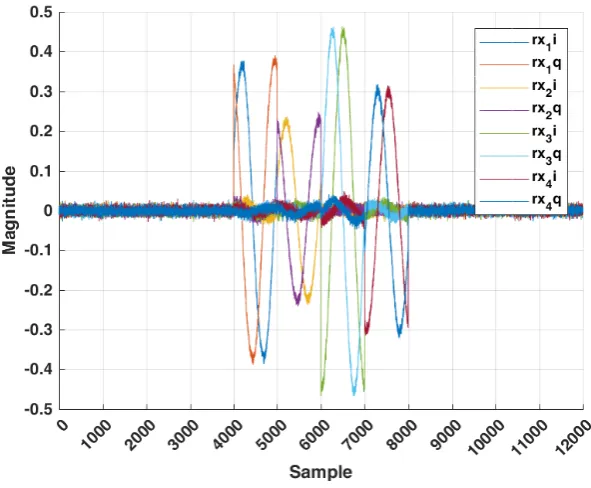
5.1.2 Results

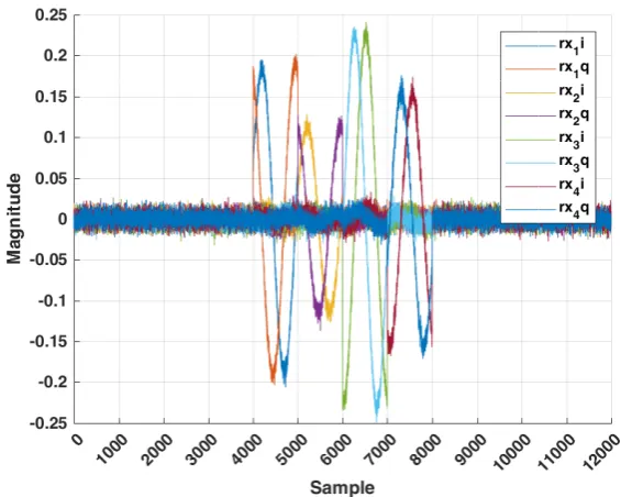
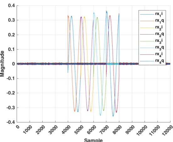
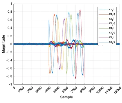
Figures 5.3 and 5.4 show both the transmitted pilot signal and the captured response of the receiver array. The way in which the amplitudes vary between the various receiver antennas is remarkable. Some variation in amplitude can be explained by constructive and destructive inter-ference, due to coupling between the antennas and due to shadowing effects, but the amount of variation shown in figure 5.4 exceeds realistic values for these phenomena. Moreover, the ampli-tude that is significantly larger than the others coincides with the antenna that is transmitting at that specific interval of time. During sample frametx2 (the interval of samples between 5000

and 6000), the amplitudes ofrx2 are larger than those of the other receiver antennas. During

these samples only tx2 is active. This raises the suspicion that there exists coupling between

the transmitter and receiver pairs of which the transfer is stronger than the transfer of the EM signals between the arrays.

The observed behavior of figure 5.4 affects the underlying techniques of spatial multiplex-ing. Table 5.1 shows the singular values with their respective condition ratios. Because a much stronger transfer exists between each of the receiver and transmitter antenna pairs than there exists between for instance tx1 and rx3, the coupling effectively induces a channel on its own.

The channels induced by coupling are similar to the situation that would arise when the trans-mitters would have a loopback to the receivers. The found singular values will then be more or less equal, with low condition ratios as a result.

Table 5.1: Singular Values and condition ratios of the direct path experiment.

1 2 3 4

(40)

Figure 5.3: Plot showing the in-phase- and quadrature components of the transmitted pilot signals.

Figure 5.4: Received response on the pilot signals. The dot-dashed lines indicate the sample frames, the dashed lines indicate the maximum amplitudes of the received signals during the sample frame oftx2 (5000-6000). It is shown thatrx2 has a larger amplitude thanrx1,rx3 and

(41)

Table 5.2 shows the singular values and condition ratios of the simulation for this experiment at similar noise levels. A comparison with the values of table 5.1 shows that something is off here, which is likely due to the on-chip coupling. While this situation is present, it is not useful to continue with the analysis of the results, as this would reflect only on the coupling behavior instead of spatial multiplexing.

Table 5.2: Singular Values and condition ratios of the direct path simulations.

1 2 3 4

SV 0.1253 0.0179 0.0007 0.0003 Ratio 1.000 6.995 168.8 465.3

5.1.3 Conclusion

The results show that coupling occurs between each of the transmitter and receiver pairs. This coupling most likely originates in the traces of the Printed Circuit Board (PCB) of the FM-COMMS5 board. The transfer between each respective transmitter - receiver pair (for instance

tx2 and rx2) is much larger than the transfer between other combinations of antennas (for

in-stancetx2 andrx4). This would affect the working of spatial multiplexing and therefore has to be further investigated.

5.2 Coupling

In the experiment of section 5.1 unexpected behavior was observed. The hypothesis is that coupling occurs between the transmitter and receiver pairs on the PCB. The goal of this ex-periment is to establish whether the observed response is indeed caused by coupling and to find whether the effects of this coupling can be canceled.

5.2.1 Analysis

Figure 5.4 shows the results of a direct path measurement in the anechoic chamber. When comparing rx3 with rx1 and rx2 for the samples of 6000 until 7000, it can be seen that the

amplitude difference of the ADC output values is about seven times as high (0.06 forrx1 and

rx2 compared to 0.42 for rx3). The average maximum values for the non-coupled signals are

roughly 0.03V (0.05 full scale input voltage). This is equivalent to a received power level of roughly -20dBm.

The amplitudes of the coupled signals range from 0.13V up to 0.28V (0.2 full scale input voltage to 0.44 full scale input voltage), which results in equivalent power levels of -7.5dBm up to -1dBm. With a transmitter power level of -2.5dBm and a receiver gain of 60dB, the loss of the non-coupled signals is found to be -77.5dB, which is much higher than the anticipated loss (equation 5.1). The transfer of the coupled signals is calculated to be−1 + 2.5−60 =−58.5dB

up to −7.5 + 2.5−60 =−65dB.

Gpath=GP athloss+GCableloss+GS11=−46.3−8.4−1.8 =−56.5dB (5.1)

The datasheet [18][p6] lists an isolation of 50dB between the two receiver and transmitter channels of each AD9361 chip. Although this is the isolation from tx1 to tx2 and not the

(42)

(a) Setup with the transmitter array connected.

(b) Setup with the transmitter connectors termi-nated.

Figure 5.5: The two setup configurations for the coupling experiments.

isolation of 60 dB between the transmitter and receiver channels would explain the observed coupling behavior. It does remain unclear why the uncoupled signals are 20dB weaker than anticipated.

For normal operations, a 50dB on chip isolation between various signals is sufficient. In the current case it is a problem because the actual desired signal is even weaker. In communication systems the transmitter and receiver are usually separated in space and therefore this problem would not occur. Also WiFi signals are in general half duplex and so the transmitter and re-ceiver would not be active at the same time which also prevents coupling.

5.2.2 Method

To analyze the coupling, two setups will be used, see figures 5.5a and 5.5b. In the setup of figure 5.5a the receiver antennas are removed and replaced by 50Ω termination components. The transmitter array remains connected to the transmitters to mimic live operation in the best way possible. In the setup of figure 5.5b both the receivers and the transmitters are terminated by the 50Ω termination components. This experiment is carried out to see whether these ter-mination components have any influence on the coupling itself.

(43)

[image:43.595.143.439.99.343.2]

Figure 5.6: Sampled coupling signals using 10dB transmitter attenuation and 60dB receiver gain at 2.45GHz using termination components for the receiver connectors.

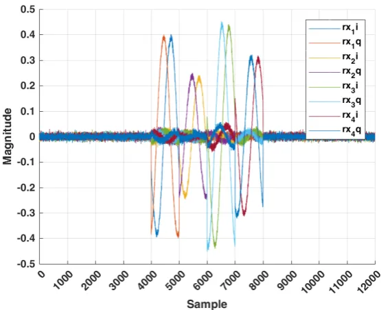
5.2.3 Results

Figure 5.6 shows the captured signals for the setup of figure 5.5a at a frequency of 2.45GHz, with 10dB transmitter attenuation and a receiver gain of 60dB1_.

It is observed that there is a transfer from transmitter to receiver even though the receiver has no antennas connected to it. It is also found that the coupling does not seem to be isolated to the respective channel pairs. Some coupling can be observed between tx1 to rx2 and also

betweentx1 torx4, even thoughtx1 is created by the first AD9361 chip andrx4 is received by

the second AD9361 chip.

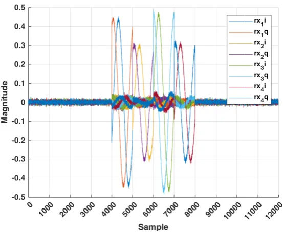
Another assumption was that the coupling was linearly dependent on the transmitted power. Figure 5.7 shows the results from a situation in which the transmitter is attenuated by an ad-ditional 6dB. The complete configuration then lists a transmitter attenuation of 16dB and a receiver gain of 60dB at a frequency of 2.45GHz.

Figure 5.7 shows that the sampled amplitude is approximately half of that of figure 5.6. As the values shown are the sampled voltages of the ADC, this indeed corresponds to the 6dB additional attenuation in power. The most obvious solution, apart from separating the receiver from the transmitter, would thus be to reduce the transmitted power. This would linearly reduce the coupling effects while the actual transmitted signals could be amplified to desired power levels externally. This would require external amplifiers that are capable of operating at 2.45GHz.

Looking again at figure 5.7 it is also promising that the phases of the measurements seem to remain constant. This would open up the possibility to cancel the coupling. A calibration

(44)

Figure 5.7: Sampled coupling signals using 16dB transmitter attenuation and 60dB receiver gain at 2.45GHz using termination components for the receiver connectors.

measurement could be taken without antennas, which could then be used to cancel the coupling during the actual experiments.

The transmitter antennas are now replaced with 50Ω termination components. The reason-ing behind this is that if the couplreason-ing effects change, the couplreason-ing is likely to be dependent on the impedance that is connected to the SMA connector. If it is not, the coupling is likely to origin earlier in the transceiver chain. Figure 5.8 shows the result of replacing the antennas at the receiver and transmitter with 50Ω termination components.

[image:44.595.147.430.97.323.2]

Comparing figure 5.8 with figure 5.6 it is observed that the coupling effects have indeed changed. If the peak of the quadrature component is taken as a reference, the respective changes of tables 5.3 and 5.4 can be determined in the amplitude and phase.

Table 5.3: Locations and the values of the maximum amplitude for each channel for the two setups of figure 5.5. The row labeled ‘Array’ denotes the peaks for the setup of figure 5.5a and ‘Terminated 50Ω’ denotes the peaks for figure 5.5b.

rx1q rx2q rx3q rx4q

(45)

[image:45.595.152.430.97.323.2]

Figure 5.8: Sampled coupling signals using 10dB transmitter attenuation and 60dB receiver gain at 2.45GHz using termination components on both transmitter and receiver.

Table 5.4: Phase shifts of table 5.3 expressed in degrees instead of samples. Values shown are the phase shift for the setup of figure 5.5a with respect to the phase of the signals of the setup of figure 5.5b

rx1 rx2 rx3 rx4

Phase difference -182° -179° -81° -96°

The results show that the amplitudes of the signals do not change much, but the phase does. This implies that it will be very difficult to cancel the coupling effects because they are not constant when changing the load. To be able to cancel the coupling, a calibration mea-surement should be carried out whilst both the arrays are connected and meanwhile preventing the broadcast signals to arrive at the other array. This would be practically impossible in any realistic situation.

Every measurement shown so far has been repeated three times in quick succession. These measurements show, apart from changes contributed to noise, no difference with respect to one another. However, figures 5.9 and 5.10 show what happens if the FMCOMMS5 board is tem-porarily disabled by setting the Enable State Machine (ENSM) mode tosleep and back tofdd2

in between measurements.

From the results, it is observed that the amplitude has no significant change. The phase does show a significant change. Moreover, it shows the same behavior that was mentioned earlier when comparing the measurements of the setups of figures 5.5a and 5.5b. Earlier this behavior was contributed to a changing load, but it is apparently linked to the start-up behavior of the device.

An explanation for this behavior can be found in the block diagram of the AD9361 chip of

(46)

[image:46.595.154.430.133.359.2]

Figure 5.9: Coupling measurement after re-initiating the device for the first time.

[image:46.595.153.430.478.705.2]

(47)

figure 4.2. In the middle on the left the generation of the modulator signals is shown. Even though the signals are generated by the same crystal, the synthesizers that create the Local Oscillator (LO) signals used for modulation and demodulation are distinct devices[22][p18]]. This enables the simultaneous usage of the transmitter chain and the receiver chain at dif-ferent frequencies. This, however, also implies that the LO signals are not guaranteed to be synchronized, with the result that after every synthesizer power-up there is an arbitrary phase difference between the two LO signals. This phase difference then causes a phase difference in the received signals.

[image:47.595.153.429.406.633.2]

To test this theory, the experiment is repeated with four loopback cables between each re-spective transmitter and receiver pair3. The results shown in figures 5.11 and 5.12 show that the phase difference also occurs in this situation. This troubles the ability to cancel the coupling effects as this phase difference has to be calibrated after every power-up sequence. A solution would be to use an external oscillator for the LO synthesizer signals. With the external os-cillator used for both modulation and demodulation, there should not be variable phase shift anymore, as they are all performed by the same LO signal.

Figure 5.11: Measurement with loopback cables after booting up the first time.

(48)

[image:48.595.154.430.95.321.2]

Figure 5.12: Measurement with loopback cables after rebooting the device.

Finally also the dependability on frequency has been looked into. Figures 5.13a, 5.13b and 5.13c show the response for the setup with both the transmitter and the receiver 50Ω terminated for frequencies of 800MHz, 2.45 GHz and 5GHz. The large differences in amplitude show that the coupling is also dependent on the frequency.

5.2.4 Conclusion

Experiments have shown that coupling occurs inside the PCB of the FMCOMMS5. The re-jection of the PCB between the transmitter and receiver pairs is found to be inadequate for the purpose of the experiments. The rejection is estimated to be in the 50-60dB range. The complete path loss of the setup exceeds that, causing the coupling inside the PCB to be larger than the desired signals.

It was found that the design of the hardware made it too troublesome to obtain a situation where it was possible to cancel the coupling. The option of decreasing the transmitted power on the board is preferred. External amplifiers can then be used to achieve the desired power levels.

A lack of synchronization between the LO signals of the synthesizers introduces phase off-sets to the signals. These offoff-sets remain and will be taken into account by the system during the estimation of the channel. This will make the analysis of the singular vectors much more troublesome.

5.3 External amplification

(49)

(a) Coupling results for a LO frequency of 800MHz. (b) Coupling results for a LO frequency of 2.45GHz.

[image:49.595.194.391.427.593.2]

(c) Coupling results for a LO frequency of 5GHz.

(50)

and external amplifiers will be used.

The experiments will once again be carried out in the anechoic chamber and will have two goals. The first goal is to verify that the coupling effect has been decreased enough to do sen-sible measurements. The second goal of the experiment is to confirm the theories presented in chapter 2 by relating the simulations of chapter 3 to the processed results of the experiments.

5.3.1 Method

During the time of the experiments, the only amplifiers that were available, were the LNA-1440[23]. This Low Noise Amplifier (LNA) has an operating range of 10kHz up to 1400MHz. To be able to use these, the frequency of the LO signals has to be lowered to 1400MHz. Also a modification to the antenna array is required, as a linear phased array antenna works best with the antennas spaced at half a wavelength. Both the transmitter and receiver array are modified in such a way that the antennas are approximately 107mm apart, which coincides with half a wavelength at 1400MHz.

This modification also affects the measurements in the anechoic chamber. A decrease in frequency will increase the radius in which near field effects have to be taken into consideration. To be able to neglect near-field effects, the distance between the antenna arrays should be larger than 2D2/λ, where D is the largest dimension of the radiator and λ is the wavelength [24][p34]. The largest dimension of the array is the distance fromtx1 totx4 which is 3·0.107m.

Equation 5.2 shows that after the modifications the receiver array is still spaced far enough to be considered in the far-field region.

Rf arf ield=

2·0.3212

0.107 = 1.92m (5.2)

For the experiment the setup of figure 5.2 is used. The arrays are placed in the anechoic chamber at a distance of 2.9m from one another. Training signals are sent at a frequency of 1400Mhz with a transmitter power level of -42.5dBm (50dB attenuation). External amplifiers of the type LNA-1440 are used to provide a gain of 40dB. The experiments are all repeated four times for various situations. These situations vary with respect to the angle of the receiver array, the presence of reflective surfaces and the presence of an interferer. Because external am-plification is required, the system platform is now placed outside the anechoic chamber. Both the transmitter and the receiver array are connected by SMA cables of six meters long.

5.3.2 Results

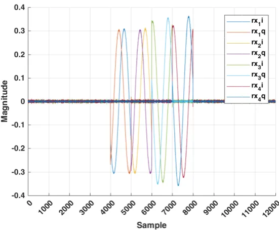
In figure 5.14 the resulting received signals are shown for the most basic setup possible. Only the two antenna arrays are present and neither of them is rotated (figure 5.2). Figure 5.14 shows that the signals received for each sample frame have roughly the same phase. This is the expected behavior when there is only a direct path between transmitter and receiver and the distance between every antenna pair is about the same.

It is also observed that during sample frame tx2 the signals are a bit weaker and messier than during the other sample frames. This is most likely caused by the fact that antenna tx2

(51)

[image:51.595.149.430.95.321.2]

Figure 5.14: Received signals of a setup without any reflection surfaces added and both receivers 0° rotated.

More striking, however, is that sample frames tx3 and tx4 seem to have a phase offset of

180°compared to sample frame tx2 and an offset of -90° with respect to sample frame tx1.

The phase shift oftx1 with respect to tx3 and tx4 can be explained by looking again at the

synthesizers. Based on the experiment where the coupling between the transmitter and receiver pairs was investigated, it was mentioned that the built in synthesizers of each AD9361 chip for the transmitters and receivers are not phase locked. In figure 4.2 it is shown that this is also not the case for the synthesizer used for modulating tx1 and tx2 (AD9361 A) with respect to

the synthesizer that is used for channelstx3 and tx4 (AD9361 B). A phase offset of 180° of the

transmit synthesizer of AD9361 B with respect to AD9361 A, results in the pilot signals also having the same phase offset for the samples during the 6001-8000 interval.

This, however, does not explain the phase shift of sample frame tx2. This transmitter is

supposed to use the same LO signals for both modulation as demodulation as tx1 and should

therefore have roughly the same phase. It is most likely that the antennatx2 is not performing

properly because the received amplitudes are also significantly smaller than during the other sample frames. This again does not impair the effects of spatial multiplexing (these offsets are take into account during training), but does complicate the analysis. This once again proves the need of a careful characterization of the antenna paths for a proper analysis.