warwick.ac.uk/lib-publications
A Thesis Submitted for the Degree of PhD at the University of Warwick
Permanent WRAP URL:
http://wrap.warwick.ac.uk/109059/
Copyright and reuse:
This thesis is made available online and is protected by original copyright.
Please scroll down to view the document itself.
Please refer to the repository record for this item for information to help you to cite it.
Our policy information is available from the repository home page.
The Development and Application of
Optically Generated Spatial Carrier Fringes
for the Quantitative Measurement of
Flowfields and Solid Surfaces
Ping Hai Chan
Department of Engineering, University of Warwick
This thesis is submitted for the degree of Doctor of Philosophy
Declaration
This thesis is presented in accordance with the regulations for the degree
of Doctor of Philosophy. It has been composed by myself and has not been
submitted in any previous application for any degree. The work described in
this thesis has been done by myself except where references are made to the
Acknowledgements
I would like to give my special thanks to Dr. P. J. Bryanston-Cross, my
supervisor who has made this research possible, for his precious guidance
and constant support. I wish to express my sincere gratitude to Prof. J.
O. Flower for his time and effort to solve my personal problem during my
research.
I would like to acknowledge the help and support of all members o f our
research team, especially Dr. T. R. Judge and Mr. Z. Zhang.
I would also like to think those who aided in proof reading this thesis;
especially Mr. Geoff Davis. Finally, my special thanks go to my family and
my friends, Miss Yong-Ying Xiao and Mr. Sai-Tim Leung. Without whose
support and encouragement, I could not have completed my thesis.
Abstract
There are two main approaches to fringe pattern analysis: spatial carrier
and temporal carrier. The phase-stepping (PS) method plays a prominent
part in the temporal carrier approach. The principal technique of the spa
tial carrier approach is the discrete Fourier transform (D FT) method. In
this thesis, both methods are reviewed and illustrated with examples. The
problems associated with these methods are discussed. The effect of weight
ing function and filtering window on the accuracy of the DFT method is
investigated. A review o f the minimum spanning tree approach to phase
unwrapping is presented.
A new fringe evaluation technique has been explored. The technique
combines the computational simplicity o f the PS method with the single
image analysis capability o f the DFT method. This technique is implemented
over two steps. Firstly, a fringe pattern with spatial carrier is subdivided into
three component images. Then, the phase is calculated by a three phase step
algorithm from these images. A computer simulation has been undertaken to
demonstrate the theory and to analyse the systematic errors. Applications
in the analysis of the transonic flow-fields are presented.
The Fourier Transform Profilometry (FTP ) decodes the 3-D shape in
formation from the phase stored in a 2-D image o f an object onto which a
Ronchi grating is projected. Two different optical geometries used in the
FTP have been compared. The phase information can be separated from
the image signal by either the phase subtraction method or the spectrum
Contents
1 Introduction 1
1.1 An Overview of Fringe Pattern Analysis T echniques... 2
1.2 Brief Review of Optical Principles... 3
1.2.1 Harmonic Wave Motion and L ig h t... 3
1.3 Interference of Light ... 5
1.4 Polarization of L i g h t ... 7
2 Fringe Pattern Analysis by Discrete Fourier Transform Tech niques 11 2.1 In trodu ction ... 11
2.2 Discrete Fourier Transform T e ch n iq u e s ... 12
2.2.1 1-D Discrete Fourier Transform T e c h n iq u e ... 12
2.2.2 2-D Discrete Fourier Transform T e c h n iq u e ... 16
2.3 Other Fourier Transform Techniques ... 20
2.4 The Problems Associated with Discrete Fourier Transform Techniques... 24
2.4.1 Influence of N o is e ...24
2.4.2 Fringe Discontinuities... 24
2.4.3 Other Error S o u r c e s ... 26
2.5 Application Example of Discrete Fourier Transform Techniques 27 3 The Effect of Weighting Function and Filtering W indow on Accuracy of 1-D Fourier FVinge Analysis 38 3.1 In trodu ction ... 38
3.2 The Characteristics of 1-D Weighting Function Used in the E x p e rim e n t... 39
\
3.2.1 Summary of 1-D Weighting Functions...40
3.3 The Joint Effect of 1-D Weighting Function and Filtering Win dow ... 46
3.4 D iscu ssion ... 52
4 The Effect of Weighting Function and Filtering Window on Accuracy of 2-D Fourier Fringe Analysis 54 4.1 In trodu ction ... 54
4.2 Formation of 2-D Weighting F u n ction ... 55
4.3 The Joint Effect of 2-D Weighting Function and Filtering Win dow ... 56
4.4 D iscu ssion ...64
5 Fringe Pattern Analysis by Phase-stepping Techniques 68 5.1 Introduction...68
5.2 Phase-stepping Measurement A lg orith m s... 70
5.2.1 Three Phase Step A lg orith m ... 70
5.2.2 Four Phase Step A lg o r i t h m ... 71
5.2.3 Carre’s Algorithm ... 72
5.2.4 Five Phase Step A lgorith m ... 73
5.2.5 N + l Phase Step A lg o rith m s... 74
5.2.6 ” 2+ 1 ” A lg o rith m ... 75
5.3 The Problem associated with Phase-stepping Techniques . . . 76
5.3.1 Phase Shifter Errors ... 76
5.3.2 Detector Nonlinearities... 77
5.3.3 Intensity Error ... 78
5.4 Application Example of Phase-stepping T e ch n iq u e s ... 79
6 Fringe Pattern Analysis by Spatial Phase-stepping Technique
86
6.1 In trodu ction ...866.2 Previous Research W ork s... 87
6.2.1 Spatial Version of the Phase-stepping Technique . . . . 87
6.2.2 Spatial-carrier Phase Stepping Technique...90
6.4 The Error A n a ly s is ...93
6.5 Application Examples o f the Spatial Phase-stepping Technique 99 7 The Minimum Spanning Tree Approach to Phase Unwrap ping 112 7.1 Introduction... 112
7.2 A Brief Overview of Phase Unwrapping A lgorith m ... 114
7.3 Graph Theory and A lg orith m s... 115
7.3.1 The Basic C on cep ts...115
7.3.2 Minimum Spanning T r e e s ... 117
7.4 Hierarchical Phase Unwrapping Strategy Using M S T ... 119
7.4.1 Pixel Level Phase Unwrapping... 120
7.4.2 Tile Level Phase U n w ra p p in g ...122
7.4.3 Selection of an Appropriate Tile S i z e ...124
7.5 D iscu ssion ... 127
8 Theoretical Analysis of Fourier Transform Profilometry 132 8.1 Introduction...132
8.2 Optical Geometry of F T P ...133
8.2.1 Crossed-Optical-Axis G e o m e t r y ... 133
8.2.2 Parallel-Optical-Axis G e o m e t r y ... 135
8.3 Comparison of Different Optical G e o m e t r y ...136
8.4 The Fourier Transform Profilom etry...139
8.4.1 The Phase Subtraction M e t h o d ... 140
8.4.2 The Spectrum Shift M e t h o d ... 141
8.4.3 Phase-Height C on version ... 142
9 Limitations of Fourier Transform Profilometry 144 9.1 Maximum Range of M easu rem en t... 144
9.2 Object Size and Depth o f F i e l d ... 147
9.3 Measurement S e n s itiv ity ... 147
9.3.1 Charge-coupled Devices C am era ... 148
9.3.2 Measurement Sensitivity of FTP Using CCD Camera . 150
10 Optical Measurement o f 3 -D Object Profile by F T P 154
\
10.1 Introduction...154
10.2 Scene Illumination T e c h n iq u e ... 154
10.2.1 Basic Types o f Illu m in a to rs... 155
10.2.2 Illumination Techniques for F T P ...156
10.3 Comparision of Different Phase Extraction M e th o d s ...157
10.3.1 Results of the Phase Subtraction M e th o d ...159
10.3.2 Results of the Spectrum Shift Method ...163
10.3.3 Phase Subtraction Method Vs Spectrum Shift Method 165 11 Conclusion and Further Work 169 11.1 C onclusion...169
11.2 Further W o r k ...174
11.2.1 The Further Work o f Spatial Phase-stepping Technique 174 11.2.2 Fringe Pattern Analysis by Walsh T ransform ...174
A List of Publications Based on the Thesis 177 B Theoretical Aspect of Fluid Flow Measurement 178 C M atlab M-files for F TP 182 C .l M-file o f phase subtraction m e t h o d ... 182
List of Figures
1.1 A transverse wave travelling in the Z d irection ... 4
1.2 The wave resolved into two mutually perpendicular com po
nents ... 5
2.1 The computer generated interferogram o f a vibratory annu
lar disk with carrier fr in g e ... 13
2.2 The computer generated tilt-free interferogram of a vibra
tory annular d i s k ... 14
2.3 A spatial frequency spectrum of raster 256 of the computer
generated interferogram with carrier frin g e ... 15
2.4 (a) The extracted side lobe; (b) The extracted side lobe
translated by the carrier frequency to the origin position . . 16
2.5 The computer generated interferogram o f a vibratory annu
lar disk with non-vertical carrier fr in g e ... 17
2.6 The Fourier transform plane o f the interferogram with non
vertical carrier frin g e ... 18
2.7 The side lobe isolated by a 2-D filter in Fourier transform
plane ... 19
2.8 The isolated side lobe translated by the 2-D carrier fre
quency to the origin position ... 19
2.9 The cross grating for simultaneously measuring two direc
tional d e fo r m a tio n ... 20
2.10 Michelson-type two-channel interferometer [10] ... 21
2.11 Data acquisition process [10] 22
2.12 The Spatio-temporal interferogram [1 0 ]...22
2.13 Spatio-temporal frequency spectra of Fig. 2.12 [ 1 0 ] ... 23
2.14 The phase distributions of two different gas flow fields [10] . 23
\
2.15 The extrapolated interferogram ... 25
2.16 The schematic diagram of the experiment set-up ...28
2.17 The interferogram of the hot soldering iron ... 29
2.18 The wrapped phase map o f the hot soldering i r o n ...30
2.19 The 3-D mesh plot solution of the hot soldering iron . . . . 31
2.20 The experiment set-up to visualise the tranic jet wake flow . 31 2.21 The lateral shearing interferogram with flow f i e l d ...33
2.22 The contour plot of 2-D DFT of Figure 2.21 34 2.23 The phase map of the transonic flow f i e l d ...34
2.24 The contour plot of retrieved p h a s e ... 35
3.1 Periodic extension of observed one dimensional signal with d is co n tin u ity ... 39
3.2 The Rectangle weighting fu n ction ...41
3.3 The frequency response of the Rectangle weighting function 41 3.4 The Hanning weighting function ...42
3.5 The frequency response o f the Hanning weighting function . 42 3.6 The Papoulis weighting function ...43
3.7 The frequency response o f the Papoulis weighting function . 43 3.8 The Hamming weighting fu n ctio n ...44
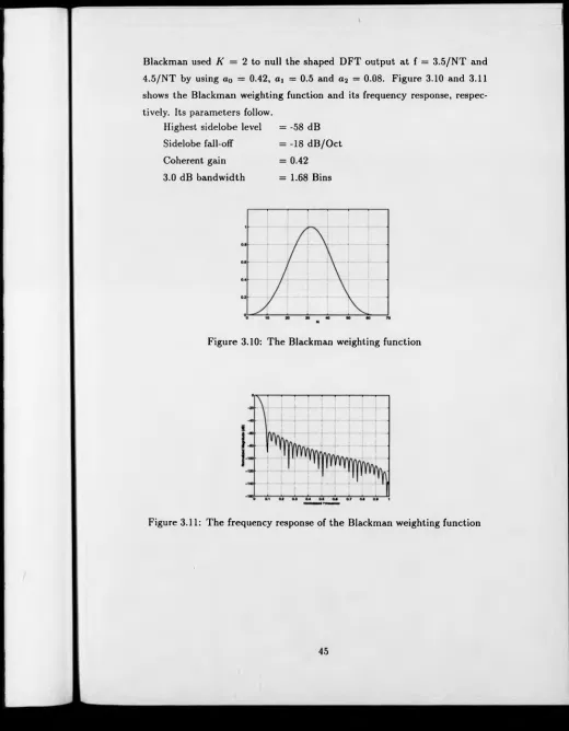
3.9 The frequency response of the Hamming weighting function 44 3.10 The Blackman weighting fu n ction ...45
3.11 The frequency response of the Blackman weighting function 45 3.12 The 3-D plot of the computer generated interferogram’s phase d is t r ib u t io n ...47
3.13 The computer generated interferogram ... 48
3.14 The mean absolute value o f the full field errors ... 49
3.15 The maximum absolute value of the full field e r r o r s ...49
3.16 The mean absolute value o f the errors after five pixels are masked o u t ...50
3.17 The maximum absolute value of the errors after five pixels are masked o u t ...50
3.18 The mean absolute value o f the errors after ten pixels are masked o u t ... 51
\
3.19 The maximum absolute value of the errors after ten pixels
are masked o u t ... 51
4.1 Two dimensional discrete sig n a l...55
4.2 Two dimensional periodic extension of signal shown in fig
ure 4 .1 ... 55
4.3 The contour plot of the frequency responses of the Hamming
outer-product w in d o w ...56
4.4 The first quadrant mesh plot of the frequency responses o f
the Hamming outer-product w i n d o w ... 57
4.5 The contour plot of the frequency responses of the Hamming
circularly rotated w in d o w ... 57
4.6 The first quadrant mesh plot of the frequency responses o f
the Hamming circularly rotated w i n d o w ...58
4.7 The contour plot of the frequency responses o f the Papoulis
outer-product w in d o w ...58
4.8 The first quadrant mesh plot of the frequency responses o f
the Papoulis outer-product w in d o w ... 59
4.9 The contour plot of the frequency responses of the Papoulis
circularly rotated w in d o w ...59
4.10 The first quadrant mesh plot of the frequency responses of
the Papoulis circularly rotated w in d o w ... 60
4.11 The contour plot of the frequency responses of the Rectangle
w i n d o w ... 60
4.12 The first quadrant mesh plot of the frequency responses o f
the Rectangle w in d o w ... 61
4.13 The computer generated interferogram with non-vertical fringe 62
4.14 The mean absolute value of the full field e r r o r s ... 63
4.15 The maximum absolute value of the full field e r r o r s ... 63
4.16 The mean absolute value o f the errors after five pixels are
masked o u t ...64
4.17 The maximum absolute value of the errors after five pixels
are masked o u t ...65
4.18 The mean absolute value o f the errors after ten pixels are
masked o u t ... 65
4.19 The maximum absolute value of the errors after ten pixels
are masked o u t ... 66
5.1 First holographic interferogram of vibrating board ...80
5.2 Second holographic interferogram of vibrating board . . . . 80
5.3 Third holographic interferogram of vibrating b o a r d ... 81
5.4 The detected low modulation points for vibrating board . . 82
5.5 The wrapped phase map for vibrating b o a r d ... 82
5.6 The tiles and connection of the wrapped phase map for vi
brating b o a r d ... 83
5.7 The mesh plot of unwrapped phase for vibrating board . . . 83
6.1 Schematic respresentation o f temporal (a) and spatial (b)
version o f phase-stepping techn iqu e... 88
6.2 The three-channel polarisation interferometer; BS 1-3, beam
splitter; P, polarisator; Q W R, quarter-wave retarder; C 1-3,
CCD cam eras... 89
6.3 The colour projection moire system with RGB camera [6] . 89
6.4 The multi-channel radial-shear interferometer [ 9 ] ...90
6.5 The three images split from the interferogram with M =3
(pixel samples in steps of 6 in y a x is )... 95
6.6 The wrapped phase map o f the interferogram with M =3
(pixel samples in steps of 6 in y axis) ...96
6.7 The contour plot of phase error of the interferogram with
M = 3 ... 96
6.8 The three images split from the interferogram with M=1.5
(pixel samples in steps of 6 in y a x is )...97
6.9 The wrapped phase map o f the interferogram with M=1.5
(pixel samples in steps of 6 in y a x is )...98
6.10 The contour plot of phase error of the interferogram with
M=1.5
\
V
6.11 The error analysis o f the interferogram with M=3 a) The
theoretical phase value of raster line 512, b) The error map
of raster line 5 1 2 ...99
6.12 The error analysis o f the interferogram with M=1.5 a) The theoretical phase value of raster line 512, b) The error map o f raster line 5 1 2 ... 100
6.13 The error analysis o f the interferogram with M =3 a) The theoretical phase value of raster line 256, b) The error map of raster line 256 ... 100
6.14 The error analysis o f the interferogram with M=1.5 a) The theoretical phase value of raster line 256, b) The error map of raster line 256 ... 101
6.15 The interferogram o f a 2-D transonic flow field ... 102
6.16 The three images split from the interferogram of a 2-D tran sonic flow f i e l d ...103
6.17 The wrapped phase map of 2-D transonic flow field com puted by SPS te c h n iq u e ...104
6.18 The wrapped phase map of 2-D transonic flow field com puted by DFT technique...104
6.19 The contour plot o f unwrapped phase o f 2-D transonic flow field retrieved by SPS technique...105
6.20 The contour plot o f unwrapped phase o f 2-D transonic flow field retrieved by D F T te c h n iq u e ...105
6.21 The interferogram o f transonic flow around a NACA 0012 aerofoil at Mach 0 . 8 ... 107
6.22 The three images subdivided from Figure 6.21 108 6.23 The wrapped phase map of Figure 6.21 computed by SPS te c h n iq u e ...109
6.24 The wrapped phase map of the low resolution image com puted by DFT technique...109
7.1 A wrapped phase map computed by D F T m eth od ... 113
7.2 The graph G = (V , E ) ... 116
7.3 The subgraph of graph G = (V , E ) ...117
7.4 Four different circuits ... 118
7.5 An example o f a t r e e ... 118
7.6 A minimum spanning tree in a weighted graph ...119
7.7 Computation of edge weights at pixel le v e l... 121
7.8 A tiled section of the wrapped phase m a p ...123
7.9 Tiles being arranged at their correct height offsets [1] . . . . 124
7.10 The tile with one badly disrupted fringe edge [1] 125 7.11 The tile with two badly disrupted fringe edge [ 1 ] ...126
7.12 The adaptive tile sizing a p p ro a ch ... 129
8.1 Crossed-optical-axis g e o m e try ... 133
8.2 Parallel-optical-axis g e o m e try ... 135
8.3 General optical geometry ...136
8.4 (A ) Spatial frequency spectra of deformed grating image for a fixed y. (B ) For spectrum shift method, only the funda mental frequency spectrum (shaded) is selected and trans lated to the origin...139
9.1 Condition for separating fundamental frequency spectrum Q i (shaded) from other s p e c t r a ...145
9.2 The cross-section diagram of a three-phase, two-bit, n-channel C C D ...148
9.3 The clock wave forms and output signal for CCD as an image sensor ... 149
9.4 CCD cells array arranged on rectangular g r i d ... 149
9.5 The parallel-optical-axis FTP using CCD c a m e r a ... 150
10.1 Basic types o f illu m in a to r... 155
10.2 Front illu m in a tio n ... 156
10.3 Offset illu m in ation ... 157
10.4 Porlarised lighting illu m in a tio n ...158
10.5 The schematic diagram of experimental s e t-u p ... 158
10.6 The image o f perturbed g r a tin g ...159
10.7 The image of Ronchi grating projected onto reference plane 160
10.8 The wrapped phase map produced by phase subtraction
m e t h o d ... 161
10.9 The 3-D plot o f the unwrapped data produced by phase
subtraction m eth od ...162
10.10 The side view of the unwrapped data produced by phase
subtraction m eth od ...162
10.11 The wrapped phase map produced by spectrum shift methodl63
10.12 The 3-D plot of the unwrapped data produced by spectrum
shift m e t h o d ... 164
10.13 The side view o f the unwrapped data produced by spectrum
shift method ... 164
10.14 The 3-D plot of the corrected unwrapped d a ta ...165
10.15 The side view o f the corrected unwrapped d a t a ...166
B .l Basic arrangement o f a Mach-Zehnder interferometer . . . .1 7 9
B.2 Cross-section of axisymmetric flow field. The light propa
gates in the Z-direction 179
\
List of Tables
5.1 The effect of harmonic order on various a lg o r ith m s ... 78
Chapter 1
Introduction
Optical metrology is a technology which covers all measurement techniques
using an optical element or aspect. There are several reasons for the use
of optical metrology. Firstly, Optical measurements are non-contact. This
property is important for the application where a measurement would be
upset by touch, or the instrument cannot reach the object. Secondly, highly
accurate measurement is possible because o f the properties of light. Finally,
optical techniques are non-destructive.
Optical metrology has experienced rapid development in recent years.
This is due to advances in laser technology coupled with the development of
electronic technology. Currently, research into optical metrology is mainly
focused on the development of low-cost high-speed analysis systems. There is
an interdependence between the design of the system and analysis techniques
used in the system. One o f the system designer’s aims is to simplify and to
automate the analysis techniques. The development of the analysis technique
requires an understanding of the theoretical aspects and the electronic devices
used in the system, as well as the algorithms employed in analysis. This is
a multidisciplinary subject, involving Physics, Electronic Engineering and
Computer Science.
In this project, several analysis techniques are studied. A new analysis
method has been developed. The main area of this study is concerned with
the method for measurement of 3-D object profile and fluid flow using spatial
carrier.
1.1
A n Overview o f Fringe Pattern Analysis
Techniques
Fringe patterns can be produced by a variety o f optical systems, for exam
ple interference of light and Moire. Reid [1] suggests that the field of fringe
analysis is now regarded by many as an independent subject. If Reid’s sug
gestion holds water, the source of the fringe pattern has little influence on the
analysis techniques. In early days, fringe analysis was carried out manually.
The processing speed of computers has been significantly improved in the
past few years. In conjunction with the development of photoelectrical de
tector technology, this hits stimulated researchers to explore automatic fringe
analysis techniques.
There are two approaches to the automatic analysis of fringe. The first
one is the intensity-based method relying on a single fringe pattern image.
Fringe tracking [2, 3, 4] is based on this approach. The fringe tracking method
usually relies on the following procedures [5]:
1. Filter the image [6].
2. Either (a) fit curves to the intensity data with a view to interpolat
ing between fringe centres [7] or (b) identify and track the intensity
maxima and/or minima with a view to skeletonising the pattern and
thereby minimising the amount o f data which must subsequently be
processed [8].
3. Number the fringe either interactively [9] or automatically [10].
4. Calculate the measurement parameter from the fringe pattern data.
The major problem associated with fringe tracking is that the information
on the sign of the retrieved phase is lost. Secondly, it is difficult to identify the
fringe orders when the fringe pattern is broken or wandered over to another
fringe pattern. Furthermore, fringe tracking also suffers from low data reso
lution as well as bad data distribution. However, the intensity-based method
may be the only applicable automatic technique for some interferograms, for
example; the fringe pattern obtained form time-average holographic vibration
The second method of automatic fringe analysis is to apply various con
cepts o f phase measuring [11, 12]. This approach can be classified into two
categories which are the temporal carrier approach and the spatial carrier
approach. The phase measuring method gives several advantages over the
intensity method. These include reduced sensitivity to the background and
contrast variations in the fringe pattern, automatic peak and valley detection
and reduced or eliminated operator interaction [13]. The detail o f different
phase measuring methods will be discussed in later chapters.
1.2
Brief Review o f Optical Principles
The optical principles are well-established. This section will summarize the
theories which are the key elements in optical metrology. The aim o f this
section is to outline the notation and approach used in this thesis. A more
detailed treatment of optical principles will be found in any standard op
tics textbook- for example references [14] - [16]. The following discussion is
derived from "Optics” edited by E. Hecht [15].
1 .2 .1
H arm onic W a v e M o tio n and Light
A wave form for which the profile is a sine curve is known as harmonic wave.
This form of wave motion is the foundation to all shapes of wave motion.
The harmonic wave can be represented concisely by using complex notation.
For example, if A is the amplitude, k is the propagation constant and 0 is
the phase constant;
^ (x,< )| (=0 = As\n(kx + 0) (1.1)
may be expressed as
i/(x,OI«=o = »[>le*(*I+#>]
(1.2)
It is usually assumed that the real part is taken so Eq. 1.2 is simply written
as
U (x,t)\t=0 = Ae,(fcx+#* (1.3)
By replacing x by (x — vt), Eq. 1.1 is transformed into a progressive wave
\
travelling at speed v in the positive x-direction and can be expressed as
i /( x ,t ) = Asin[A:(x — vt) + 9] (1.4)
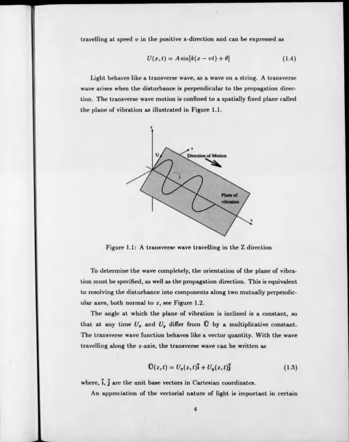
Light behaves like a transverse wave, as a wave on a string. A transverse
wave arises when the disturbance is perpendicular to the propagation direc
tion. The transverse wave motion is confined to a spatially fixed plane called
the plane of vibration as illustrated in Figure 1.1.
Figure 1.1: A transverse wave travelling in the Z direction
To determine the wave completely, the orientation of the plane of vibra
tion must be specified, as well as the propagation direction. This is equivalent
to resolving the disturbance into components along two mutually perpendic
ular axes, both normal to z, see Figure 1.2.
The angle at which the plane of vibration is inclined is a constant, so
that at any time Ux and Uv differ from U by a multiplicative constant.
The transverse wave function behaves like a vector quantity. With the wave
travelling along the z-axis, the transverse wave can be written as
0 ( z , i ) = t/*(z, i)T + Uy( z , t ) i (1.5)
where, I, J are the unit base vectors in Cartesian coordinates.
[image:21.561.8.519.18.664.2]\
Figure 1.2: The wave resolved into two mutually perpendicular components
applications, such as the polariscope. However, there are many instances in
which it is not necessary to be concerned with the vector nature o f light.
For example, if all the lightwaves propagate along the same line and share
a common constant plane o f vibration, they may each be described in terms
o f one electric-field component. This leads to a simple and very useful scalar
theory. A scalar harmonic plane wave, moving in the z direction, is expressed
as
U (z,t) = Ae^k,±u,) (1.6)
where ui is the angular frequency.
1.3
Interference o f Light
The principle of superposition of waves states that if two or more wavefronts
are travelling past a given point, the total amplitude of the displacement
at that point is given by the vector sum of the individual constituent dis
turbances. It is the basis of the light interference theory because optical
interference may be thought of as an interaction of two or more lightwaves.
[image:22.562.3.518.19.667.2]y
Given two scalar light waves described by
Ui = At sin(uit -1- a j) (1.7)
and
Ui = A2sin(w< + a 2) (1.8)
overlapping in space, the resultant disturbance is the linear superposition of
the waves. Therefore
U = U i + U3
The intensity, which is the observable quantity, becomes
/ = \U\2
= \Ui+Ui\2
= A] + A\ + 2 Ai/12Co s(q i — <*2)
— It -f- 1 2 -I" 2\JI\ 1% cos S (1.9)
where 6, which is equal to ( « 1 — a 2), is the phase difference arising from a
combined path-length and initial phase-angle difference. The 2\J I \ ¡2 cos 6 is
known as the interference term. At various points in space, the resultant
intensity varies and depends on the value o f the interference term. When
6 = (2n + l)?r, n = 0 ,1,2, • • •
cos 6 = — 1 and the resultant intensity reaches its minima. The two waves
are 180° out of phase which is referred to as total destructive interference.
When
6 = 2nn, n = 0 ,1 ,2 , • • •
cos 6 = 1 and the resultant intensity reaches its maxima. The two waves are
in phase which is referred to as total constructive interference. For two waves
of equal intensity, 70 = I\ = h , Equation 1.9 becomes
\
so that the resultant intensity varies between 0 and 4 /0.
In developing Eq. 1.9, It is assumed that the phase difference, ¿, is con
stant in time. This means that U\ and U2 are assumed to have the same
fixed frequency. Ordinary light sources produce light that is a mix of pho
ton wavetrains. At each illuminated point in space there is a net field that
oscillates, for less than 10ns or so, before it changes phase. As a result, the
interference pattern produced by two ordinary light sources will randomly
shift around in space at an exceedingly rapid rate, averaging out and making
it quite impractical to observe.
The interval over which the lightwave resembles a sinusoid is a measure
o f what is called its temporal coherence. The spatial extent over which the
light wave oscillates in a regular, predictable way is called the coherence
length. To produce a stable interference pattern, the light sources must be
coherent and have the same frequency. Until the advent of the laser it was a
working principle that no individual sources could ever produce an observable
interference pattern.
1.4
Polarization o f Light
In the previous section, light is treated as a scalar quantity. However, light is
a vector quantity which is perpendicular to the direction of propagation and
with a defined orientation in space. This property is known as the polariza
tion o f light. When two harmonic light waves o f the same frequency wave
through the same region of space in the same direction, if their respective
planes o f vibration are mutually perpendicular, the orientation o f the resul
tant light wave may or may not be constant. The exact form of the resultant
light wave, i.c. its state o f polarization, will be considered in this chapter,
(liven two orthogonal light waves described by
( 1 1 1 )
0 y ( 2 ,< ) = L V i(*, " U,‘+ a,) (1.12)
\
The resultant light wave is the vector sum of these two orthogonal light
waves:
0 ( M ) = U X( M ) + U y (*,<)
= \Axei(k,- wt)ea‘
= (iAxe ~ ^ (1.13)
where
0 = a x + a v
6 = £»v — a x
In Eq. 1.13, the factor ed*l-u,() only gives the direction of propagation. e‘ a is
a common phase factor and a constant. Therefore, the orientation of U (z, <)
is completely determined by three independent quantities, i.e. ¿4*, Av and 6.
In the general case, when U (z,<) passes a plane of observation perpen
dicular to z-axis, the tip of U (z ,i) will trace out an ellipse in that plane.
A general state of polarization is therefore called clliptically polarized light.
Hecht [15] gives a mathematical derivation of the general state of polariza
tion. There are two cases of particular o f interest. When Ax = Av and
6 = ± § -1- 2m7T, where m = 0, ± 1 , ± 2 , . . . , the ellipse degenerates to a circle.
This special case represents circular polarized light. If 6 is zero or an inte
\
Bibliography
[1] G. T. Reid, "Image Processing Techniques for Fringe Pattern Analysis” ,
Proceedings of the 1st International Workshop on Automatic Processing
o f Fringe Patterns, Berlin, P. 13-20, 1989.
[2] B. L. Button, J. Cutts, B. N. Dobbins, C. J. Moxon, and C. Wykes, "The
Identification of Fringe Positions in Speckle Patterns,” Optics And Laser
Technology, vol. 17, p. 189-192, 1985.
[3] W. R. J. Funnell, "Image Processing Applied to the Interactive Analysis
of Interferometric Fringes,” Applied Optics, vol. 20, p. 3245-3249, 1981.
[4] S. Nakadate and H. Saito, "Fringe Scanning Speckle-pattern Interferom
etry” , Applied Optics, vol. 24(14), p. 2172-2180, 1985.
[5] G. T. Reid, "Automatic Fringe Pattern Analysis: A Review,” Optics
and Lasers in Engineering, vol. 7, p. 37-68, 1986/7.
[6] D. A. Chambless and J. A. Broadway, "Digital Filtering o f Speckle Pho
tography Data,” Experimental Mechanics, vol. 19, p. 286-289, 1979.
[7] J. B. Schemm and C. M. Vest, "Fringe Pattern Recognition and Inter
polation Using Non-Linear Regression Analysis," Applied Optics, vol.
22, p. 2850-2853, 1983.
[8] T. Yatagai, S. Nakadate, M . Idesawa, and H. Saito, "Autom atic Fringe
Analysis Using Digital Image Processing Techniques,” Optical Engineer
ing, vol. 21, p. 432-435, 1982.
[9] T. Yatagai, M. Idesawa, Y . Yamaashi, and M. Suzuki, "Interactive
Fringe Analysis System: Applications to Moire Contourgram and In-
terferogram,” Optical Engineering, vol. 21, p. 901-906, 1982.
\
[10] H. E. Cline, W. E. Lorensen, and A. S. Holik, "Autom atic Moire Con
touring,” Applied Optics, vol. 23, p. 1454-1459, 1984.
[11] K. Creath, ’’ Phase Measurement Interferometry Techniques” , Progress
in Optics, p. 350-393, 1988.
[12] J. Schwider, "Advanced Evaluation Techniques in Interferometry” ,
Progress in Optics, p. 272-359, 1990.
[13] R. Jozwicki, "New Contra Old Wavefront Measurement Concepts for
Interferometric Optical Testing” , Optical Engineering, Vol. 31, p. 422-
433, 1992.
[14] M. Born, and E. Wolf, "Principles of Optics” , Pergamon Press, 1970.
[15] E. Hecht, ’’ Optics” , Addison-Wealey, 1987.
[16] F. T. S. Yu, and I. C. Khoo, "Principles of Optical Engineering” , John
Chapter 2
Fringe Pattern Analysis by
Discrete Fourier Transform
Techniques
2.1
Introduction
The discrete Fourier transform (DFT) technique is classified into the spatial
carrier approach category. This analysis method, which was proposed by
Takeda et al [1], uses a single fringe image of the form
g ( x , y ) = a ( x ,y ) + b (x,y) cos[27r/0x + <j>(x, y )] (2.1)
Where f 0 is the spatial-carrier frequency, a(x, y) is the background intensity,
b (x ,y ) is the fringe amplitude and <p(x,y) is the phase to be determined.
In the case o f interferometry, these carrier fringes may be introduced by
a relatively large tilt to the reference mirror. Alternatively, a sine profile
grating may be projected onto an object to generate the carrier fringes. A
Ronchi grating may also be used to generate the carrier fringes because a
Ronchi grating can be considered as a sum of a series o f sinusoidal gratings.
The main advantage of the DFT technique is that it requires a single
frame image. This is essential for the measurements o f dynamic systems.
Another advantage of these techniques is that a special phase-shifting device
is not needed. On the another hand, the requirement of the detector array are
\
more stringent in the DFT technique. This is because the spatial distribution
of detector sensitivities must be uniform over the array [2].
2.2
Discrete Fourier Transform Techniques
2 .2 .1
1 -D Discrete Fourier T ransform Technique
One-dimensional DFT technique is proposed by Takeda et al [1], This tech
nique was extended by Macy [3] to handle two-dimensional data. Eq. 2.1 can
be rewritten in the following form for convenience o f explanation :
g ( x , y ) = a (x ,y ) + c ( x , y ) e x p ( 2 n i f 0x ) + c*(ar, y) e x p ( - 2 n i f 0x) (2.2)
with
c(x,y)
= 6^ 2’ — exp[t<ft(g,y)]where * denotes a complex conjugate. Figure 2.1, which shows a computer
generated interferogram of the form described by Eq. 2.1, is included here as
an example. It could represent an interferogram of a vibratory annular disk.
Figure 2.2 shows a computer generated tilt-free interferogram of the same
object in the Figure 2.1.
Then g ( x , y ) is Fourier transformed with respect to x by the use o f 1-
D fast Fourier transform algorithm. The Fourier transform of Eq. 2.2 with
respect to x is given by
G(/x,y) = A(fx,y) + C(fx - f0,y) + < ?* (-/, - f0,y)
(2.3)where the upper-case letters denote the Fourier spectra and f 0 is the spatial
carrier frequency in the x direction. Since a (x ,y ) , b (x ,y ) and <j>(x,y) have
frequencies which are much lower than the spatial carrier frequency / 0, the
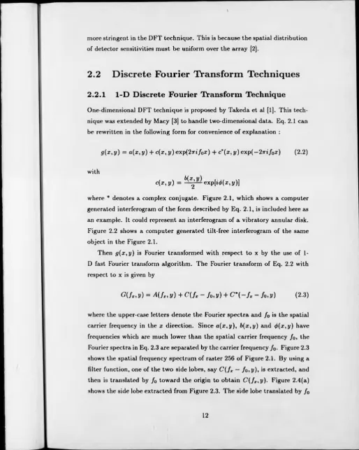
Fourier spectra in Eq. 2.3 are separated by the carrier frequency / 0. Figure 2.3
shows the spatial frequency spectrum of raster 256 o f Figure 2.1. By using a
filter function, one of the two side lobes, say
C(fx
— fo,y),
is extracted, and then is translated by f 0 toward the origin to obtain C ( f x,y). Figure 2.4(a) [image:29.561.0.515.18.662.2]T
5
■4.5
-4 ■
3.5 •
3 ■
'2.5 •
2 ■
1.5 ■
1 ■
0.5 ■
Figure 2.3: A spatial frequency spectrum o f raster 256 of the computer gen erated interferogram with carrier fringe
is shown in Figure 2.4(b). It is noted that the background variation, A (x , y ) ,
and another side lobe, C * (—/* — /o ,y ), have been filtered out in this stage.
The inverse Fourier transform of C ( f , y ) with respect to f z is computed to
obtain c(x, y). The phase may then be calculated from Eq. 2.4
The phase, 4>(x,y) in the imaginary part completely separated from the am
plitude variation, 6 (x ,y ), in the real part. The phase can also be obtained
from the equivalent operation
Since the phase calculated from Eq. 2.4 or Eq. 2.5 gives principal values
ranging from —ir to tt, <f>(x,y) is wrapped into this range. Consequently,
<t>{x, y) has discontinuities with 27T phase jumps for variations more than 2n.
<t>(x,y) is referred to as a wrapped phase map.
-0.8 - 0 .6 -0.4 -0 .2 o 0.2 0.4 o.e 0.8 Norm alized Frequency
l°g [c(x ,y )] = log[b( y > j + i<)>(x,y) (2.4)
(2.5)
[image:32.563.3.520.15.664.2]\
Figure 2.4: (a) The extracted side lobe; (b) The extracted side lobe translated by the carrier frequency to the origin position
2 .2 .2
2 -D D iscrete Fourier T ran sform Technique
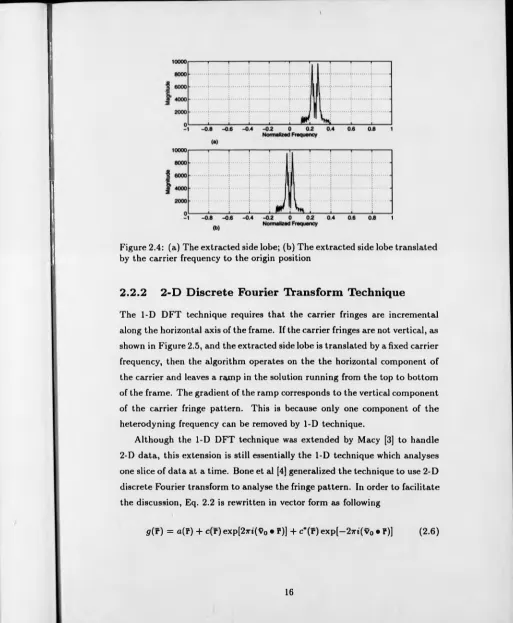
The 1-D DFT technique requires that the carrier fringes are incremental
along the horizontal axis of the frame. If the carrier fringes are not vertical, as
shown in Figure 2.5, and the extracted side lobe is translated by a fixed carrier
frequency, then the algorithm operates on the the horizontal component o f
the carrier and leaves a ramp in the solution running from the top to bottom
of the frame. The gradient of the ramp corresponds to the vertical component
of the carrier fringe pattern. This is because only one component of the
heterodyning frequency can be removed by 1-D technique.
Although the 1-D DFT technique was extended by Macy [3] to handle
2-D data, this extension is still essentially the 1-D technique which analyses
one slice o f data at a time. Bone et al [4] generalized the technique to use 2-D
discrete Fourier transform to analyse the fringe pattern. In order to facilitate
the discussion, Eq. 2.2 is rewritten in vector form as following
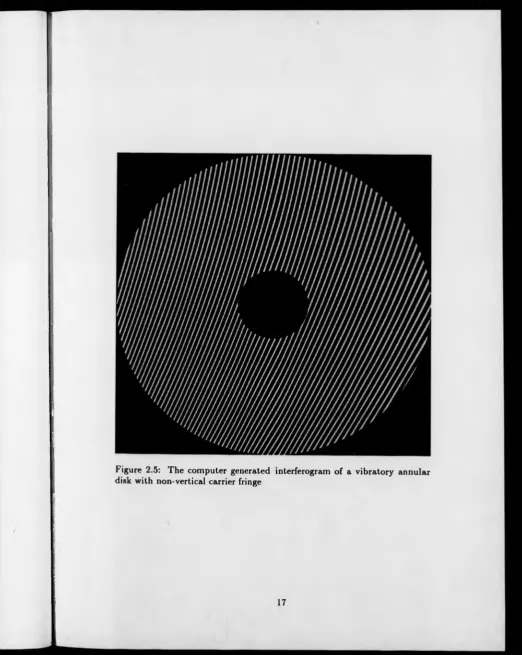
Figure 2.5: The computer generated interferogram o f a vibratory annular disk with non-vertical carrier fringe
[image:34.570.13.536.13.669.2]with
In Eq. 2.6, vector r with Cartesian coordinates ( x , y ) refers to a point on
the fringe image and v 0, which is equal to ( f To,/i/o), is the 2-D heterodyning
frequency. The 2-D Fourier transform o f g(r) becomes
functions, v is the vector frequency with component ( / * , / w).
a
^2
1
0 1
Figure 2.6: The Fourier transform plane of the interferogram with non-vertical carrier fringe
In the Fourier transform plane, all terms in Eq. 2.7 are found as strongly
peaked lobes centered at the origin and ± 9 0. Figure 2.6 shows the Fourier
transform plane o f Figure 2.5. Then, one of the two side lobes, say C (v — v 0),
is isolated in Fourier plane from the other terms in G (v ) by using a 2-D fil
tering window, and then is translated by vo toward the origin to obtain
C (v ). Figure 2.7 and Figure 2.8 shows the isolated side lobe and the trans
lated side lobe in the Fourier transform plane, respectively. The inverse 2-D
Fourier transform of C (9 ) is calculated to obtain c (f). The phase may then
be computed from either Eq. 2.4 or Eq. 2.5.
G(v) = /l(v) + C (? - v0) + C*(—v - v0) (2.7)
where the upper-case functions are the 2-D Fourier spectra o f the lower-case
x 10
Normalized Frequency (ly) _1 Normalized Frequency <f>)
Figure 2.7: The side lobe isolated by a 2-D filter in Fourier transform plane
Normalized Frequency (ly) -1 -1 Normalized Frequency (fx)
Figure 2.8: The isolated side lobe translated by the 2-D carrier frequency to the origin position
The frequency domain is an efficient way to store information in an image.
This fact has been exploited in the image compression technique [6]. In a
fringe pattern image, as revealed in Figure 2.6, the required information is
gathered round the carrier frequency and occupies a relatively small num
ber o f pixels. There are mainly two techniques, the multi-channel Fourier
fringe analysis and the spatio-temporal frequency multiplex, to utilize the
redundant space in the frequency domain so that more information can be
collected in a single fringe image.
2.3
Other Fourier Transform Techniques
Figure 2.9: The cross grating for simultaneously measuring two directional deformation
Multi-channel Fourier fringe analysis [7, 8, 9] is a technique to process
an image with more than one fringe pattern of which the spatial frequency
bandwidths must separate completely in the frequency domain. Morimoto
et al [7] made use of the multi-channel Fourier fringe analysis to measure si
multaneously the x and y directional displacement. A cross grating as shown
in Figure 2.9 is printed on the end surface o f a specimen. The intensity func
tion of the cross grating can be expressed as the sum o f two single grating
intensity functions. One grating is normal to the x axis, and another grating
is normal to the y axis. The digital image of the deformed grating is trans
formed into the frequency domain by 2-D Fourier transform. The transform
now consists of four peaks due to the fringe and a dc peak. The information
of x directional and y directional deformation can then be partitioned by
Burton et al [9] applied the multi-channel Fourier fringe analysis to the
problem of automatic phase unwrapping in the presence of surface discon
tinuities. The technique is based on the fact that if the fringe moves then
all the phase wraps will move with them, but the physical discontinuities
introduced by the surface will not move. An image that is the sum of two
fringe pattern images on the same surface is analyzed by Fourier transform
fringe analysis. This yields two wrapped-phase maps. Both wrapped phase
map would show the technique-induced discontinuities as well as the genuine
physical discontinuities. The discontinuities that remain stationary in both
wrapped phase maps are detected by image processing techniques, and hence
should be ignored during phase unwrapping.
Figure 2.10: Michelson-type two-channel interferometer [10]
Spatio-temporal frequency multiplex [10, 11] uses both spatial and tem
poral carrier frequencies. This technique enables the measurement of a phase
distribution with a wider spatial and temporal bandwidth when it combined
with the Fourier fringe analysis method. The experiment reported in Ref. [10]
is depicted here to demonstrate the principle of the technique. A two-channel
Michelson-type interferometer, which is shown in Figure 2.10 , was used in
the experiments. Two gas flow fields with different flow rate were introduced
into each of the channels. The spatial carrier frequencies were introduced
by tilting the mirrors Ml and M2. A ramp current was applied to a laser
1
1-1(1)____ 1-1(2) «-IP)
Figure 2.11: Data acquisition process [10]
diode to produce temporal carrier frequencies. Only one set of 1-D fringe
data along a fixed scanning line was taken from each frame and piled sequen
tially in a 2-D memory array to form a 2-D spatio-temporal interferogram.
Figure 2.11 explains graphically the process of data acquisition. Figure 2.12
shows a spatio-temporal interferogram with the present o f two gas flow fields.
The correlative spatio-temporal frequency spectra are shown in Figure 2.13.
The spectrum corresponding to the two different gas flow fields are indicated
by the arrow A and B. Two phase distributions retrieved from the single
spatio-temporal interferogram are presented in Figure 2.14.
\
Figure 2.13: Spatio-temporal frequency spectra o f Fig. 2.12 [10]
Figure 2.14: The phase distributions of two different gas flow fields [10]
2.4 .1
Influence o f N o ise
For a small additive white noise, the rms phase errors in heterodyne tech
niques can be calculated in term of signal-to-noise ratios (SNR). In the case
of the 1-D DFT technique, Takeda [12] gave a corresponding rms phase error
for the Fourier transform technique as
2.4
The Problems Associated with Discrete
Fourier Transform Techniques
in the frequency domain, 6 (x ,y ) is the fringe amplitude and a is the rms
value of the noise. For the two-dimensional case, Bone et al [4] gave a similar
formula for the expectation value of the rms phase error as
where m is the mean modulation amplitude.
These formulas can be interpreted as follows. In the Fourier transform
technique, the phases is obtained from the n frequency spectra spreading
over the filter passband. T h e spectra passed by the filter include n/N of the
total noise power. Therefore, the phase error is proportional to the factor,
n/N, under the small-noise assumption.
2 .4 .2
Fringe D iscontinuities
The fringe discontinuities are an important source o f error if they are not
properly taken into account. In some applications, such as in the test of
an object with a hole, the fringe abruptly disappears at the boundaries.
( 2.8)
S (x ,y ) is a SNR defined by
where n is the number of spectral sample points within the filter passband
These discontinuities cause the fringe spectra to spread out. This causes
problems not only in the Fourier transform technique, but also in the phase
unwrapping.
A way to deal with this problem is to extrapolate the fringes image. Rod-
dier et al [13] developed a systematic method o f fringe extrapolation, which
is based on Gerchberg’s iterative algorithm for analytic continuation [14]. As
an example, Figure 2.1 is extrapolated as in Figure 2.15 by adding a carrier
fringe into the boundaries.
Figure 2.15: The extrapolated interferogram
25
\
2 .4 .3
O ther Error Sources
When the frequency of detector nonlinearity is approximately equal to the
carrier frequency, detector nonlinearity is one o f the error sources. T h e re
sponse of CCD array is linear within its operation region for most C C D cam
eras in the market. Therefore, detector nonlinearity is usually not a problem
for measurement using CCD cameras. However, if the image is captured by
film, the error caused by non-linear response of the recording medium should
be taken into account. The Fourier transform techniques will interpret the
fringe distortion which is caused by the film as fringe distortion due to the
presence of the physical quantity to be measured. There are many well-
established techniques for calibrating film. Nugent [5] proposed a method
to determine the film characteristics of interferogram by measuring the de
viation of the fringe in object-free areas from pure sinusoids. This method
utilizes the fact that fringe recorded using a perfect recording medium will
be sinusoidal.
There are some errors associated with an FFT algorithm used in the
discrete Fourier transform technique. These include :
1. Aliasing.
Aliasing will occure, if the sampling frequency is lower then the Nyquist
frequency which is twice the highest frequency component o f signal to
be sampled.
2. Leakage of energy due to inappropriate truncation o f data.
This will be discused in the next two chapter.
3. The picket fence effect.
The DFT is a mechanism by which the observed singal is decomposed
into an orthognal vector space. The sines and cosines with frequency
equal to an integer multiple of 1 /NT form an othogonal basis set, where
T is the sampling interval and N T is the observation interval. From the
continuum of possible frequencies, only those which coincide with the
basis vector will project onto a single basis vector; all other frequencies
will exhibit non-zero projections on the entire basis set. This effect is
V
a frequency which is not one of the basis frequency, the picket fence
effect will occure.
2.5
Application Exam ple of Discrete Fourier
Transform Techniques
Two examples are presented in this section to demonstrate the capacity o f
the 1-D and 2-D DFT technique. The first example is to measure the change
of air density profile caused by a heat source. In this case, the heat source is
a soldering iron. In this experiment, the Twyman-Green interferometer was
used because of the availability o f the equipment. As the light wave pass
through the flow field twice, the result obtained from the Twyman-Green
interferometer should be divided by two. Figure 2.16 shows the schematic
diagram of experiment set-up. R. Jones [15] had manifested that the visibility
o f the fringe will decrease, if the ratio of the fringe spacing to the mean speckle
size approaches unity. As a result, no fringe is observed when this ratio is
approximately equal to unity. The size o f the subjective speckle is given
by [16]
, 2.4Xd
dap —
a (2.10)
where
<l,p — the subjective speckle size
A = wave length
d = the distance from the lens to the image plane
a = the diameter o f the viewing lens aperture
Thus, the viewing lens aperture should be as large as possible. The
neutral density filter is used to attenuate the light intensity evenly so that
the lens aperture can be turned to its maximum. Figure 2.17 shows the linear
fringe pattern modulated by the air density change that is caused by the heat
o f the soldering iron. The interferogram is analysed by 1-D DFT technique
since the carrier fringe is vertical. The Figure 2.18 shows the wrapped phase
map after Figure 2.17 is demodulated. The wrapped phase map is unwrapped
by the Minimum Spanning Tree approach that will be discussed later. The
\
M irror
Figure 2.16: The schematic diagram o f the experiment set-up
3-D mesh plot o f the unwrapped solution is shown in Figure 2.19.
In the second example [19], a shearing interferogram with non-vertical
carrier fringe is analysed by 2-D DFT technique. Figure 2.20 shows the
experimental set-up to visualise the transonic jet wake flow using a lateral-
shear interferometer. The collimated beam o f light passes through the flow
field and is then incident on a wedged shearing plate. The two reflected beams
are sheared laterally by the a shearing plate. The fringe pattern in the region
o f overlap is formed on the screen by the interference o f the wavefront with
its sheared duplicate. A spatial carrier fringe pattern is introduced by the
wedge angle between the two faces o f the shearing plate.
In lateral shearing interferogram with spatial carrier, the interference
fringes can be described by
g ( x , y ) = a ( x ,y ) + b ( x ,y ) c o s [ 2 r ( x f x0, y f v0) + <t>z( x , y ) + <t>(x,y)\ (2.11)
where a(x, y) and 6(x, y) represent background and modulation terms, re
spectively, (fxo, fyo) is the 2-D spatial carrier frequency introduced by wedged
geom-o
LU
N
(T
Z
CÛ
ol
p
co <
p
-co —'
Z
<
r
co <
n
LU
O
Position (pixels) Position (pixels)
Figure 2.19: The 3-D mesh plot solution of the hot soldering iron
By-pasi Nozzle Wedged Shearing
Figure 2.20: The experiment set-up to visualise the tranic jet wake flow
etry and distortion of the lenses etc. As the shear is a small fraction o f the
diameter of the wavefront, <j>x( x , y) corresponds to the derivative of the phase
change caused by the flow field along the direction of shear [17] Eq. 2.11 can
be rewritten in following form :
g ( x , y ) = a(x, y) + c ( x , y ) e x p ( 2 r j ( x f x0, y f v0)) + c ’ e x p ( - 2 n j ( x f xo , y f yo))
(2. 12)
where c(x, y) = (1 /2)b(x, y)ex p [j(<(>'( x , y)+<t>x(x, j/))] and * denotes a complex
conjugate.
Figure 2.21 shows the interferogram with the flow field. In order to cancel
the initial phase shift, a reference image is also taken prior to the presence
of the flow field. Figure 2.21 is transformed into Fourier domain by using
2-D DFT. In the Fourier Transform Plane, which is shown in Figure 2.22, all
terms in Eq. 2.12 are found as strongly peaked lobes centred at the origin
and the spatial carrier. One o f the two side lobes is isolated in Fourier plane
from the other terms by using a 2-D filtering window. The same filtering
operation was performed on both the sample and the reference images. The
phase subtraction method [18] is then employed to retrieve <j>x( x , y ) , which is
shown in Figure 2.23. It has been found that the retrieved phase is within the
27T range, and that noise has been added to the image as result o f the poor
image contrast in the the shadow region o f the by-pass nozzle. Figure 2.24
Figure 2.22: The contour plot o f 2-D DFT of Figure 2.21
(s
ie
xK
l)
uoq
iso
d
Figure 2.24: The contour plot of retrieved phase
\
Bibliography
[1] M. Takeda, H. Ina and K. Kobayashi, ” Fourier-transform Method of
Fringe Pattern Analysis for Computer-based Topography and Interfer
ometry” , J. Opt. Soc. Am., Vol. 72, p.156-160, 1982.
[2] M. Takeda, "Spatial-carrier Fringe-pattern Analysis and its Application
to Precision Interferometry and Profilometry: An Overview” , Industrial
Metrology, Vol. 1, p. 79-99, 1990.
[3] W. W. Macy, Jr., "Two-dimensional Fringe-pattern Analysis” , Appl.
Opt., Vol. 22, p. 3898-3901, 1983.
[4] D. J. Bone, H. A. Bachor, and R. J. Sandeman, "Fringe-pattern Analysis
Using a 2-D Fourier Transform” , Appl. Opt., Vol. 25, p. 1653-1659, 1986.
[5] K. A. Nugent, ” Interferogram Analysis Using an Accurate Fully Auto
matic Algorithm” , Appl. Opt., Vol. 24, p. 3101 - 3105, 1985.
[6] A. Low, "Introductory Computer Vision and Image Processing” ,
McGraw-Hill, ISBN 0-07-707403-3
[7] Y. Morimoto, Y . Seguchi and T. Higashi, "Two-dimensional Moire
Method and Brid Method Using Fourier Transform” , Experimental Me
chanics, Vol. 29, p. 339 - 404, 1989.
[8] J. M. Huntley and J. E. Field, "High Resolution Moire Photography :
Application to Dynamic Stress Analysis” , Opt. Eng., Vol. 28, p. 926 -
933, 1989.
[9] D. R. Burton and M. J. Lalor, "Multichannel Fourier Fringe Analysis as
an Aid to Automatic Phase Unwrapping” , Appl. Opt., Vol. 33, p. 2939
\
[10] M. Takeda and M. Kitoh, "Spatio-temporal Frequency-multiplex Het
erodyne Interferometry” , Proc. SPIE 1553, p. 66 - 76, 1991.
[11] M. Takeda and M. Kitoh, "Spatiotemporal Frequency Multiplex Het
erodyne Interferometry” , J. Opt. Soc. Am. A, Vol. 9, p. 1607 - p.1614,
1992.
[12] M. Takeda, "Temporal Versus Spatial Carrier Techniques for Heterodyne
Interferometry” , Proc. SPIE 814, p. 329-330, 1987.
[13] C. Roddier and F. Roddier,” Interferogram Analysis Using Fourier Trans
form Techniques” , Appl. Opt., Vol. 26, p. 1668-1673, 1987.
[14] R. W. Gerchberg, "Super-Resolution Through Error Energy Reduction” ,
Opt. Acta Vol. 21, p.709,1874.
[15] R. Jones and C. Wykes, "Holographic and Speckle Interferometry” ,
Camberidge University Press, 1989.
[16] J.W. Goodman, "Laser Speckle and Related Phenomena” , Springer-
Verlag, 1975.
[17] P. Hariharan,” Basics o f Interferometry” Academic Press Inc, 1992.
[18] M. Takeda and K. Motoh, "Fourier Transform Profilometry for Auto
matic Measurement o f 3-D Object Shapes” , Appl. Opt., Vol. 22, p. 3977-
3982, 1983.
[19] P.J. Bryanston-Cross, P.H. Chan and T.R. Judge, "Analysis of Lateral
Shearing Interferogram Using 2-D DFT Techniques” , Proc. o f Engineer
ing Applications o f Optical Diagnostic Techniques, 7th December 1994,
Cranfield University.
Chapter 3
The Effect of Weighting
Function and Filtering
W indow on Accuracy of 1-D
Fourier Fringe Analysis
3.1
Introduction
When a finite-extent sampled signal is transformed into the frequency do
main by the discrete Fourier transform (D FT ), it is assumed that the N
sample values of the finite-extent signal represent exactly one period of a pe
riodic function. The DFT implies periodicity in both the time and frequency
domains. If the signal is not a periodic function or if the observation inter
val is not equal to a integer multiple of the period of a periodic signal, the
periodic extension o f the observed signal will exhibit discontinuities at the
boundaries of the observation. The discontinuities cause a phenomena that
is called spectral leakage. The form of this discontinuity is demonstrated in
Fig 3.1.
In order to alleviate the spectral leakage, a weighting function is applied
to the data prior to the DFT. This chapter will address the effect o f weighting
function and filtering window on the performance of fringe analysis using one
Figure 3.1: Periodic extension of observed one dimensional signal with dis continuity
3.2
The Characteristics o f 1-D Weighting Func
tion U sed in the Experiment
It is often desirable to change the basic DFT output to meet the objectives
o f a particular application [1] [2] [3]. The modification can be accomplished
by applying a weighting function to the data.
A number of popular weighting functions are employed in this study.
The following sub-section, which is derived from Elliott et al [4] and Har
ris [5], presents the characteristics of these weighting functions. Firstly, the
major parameters, that will allow performance comparison between differ
ent weighting functions, are identified. A short description of each o f the
parameters follow.
Highest Sidelobe Level It is the peak ripple value of the sidelobes.
The amount of leakage into the sidelobes is directly proportional to the height
of the highest sidelobe.
Sidelobe Fall-off This parameter describes the amplitude fall ofT of
sidelobe peaks. This value is inverse proportional to the amount of leakage
into the sidelones.
Coherent Gain This is a measure o f the weighting function gain.
For a rectangle weighting function, the gain is equal to one. For any other
window, the gain is less than one due to the weighting function smoothly
going to zero near the boundaries.
3.0 dB Bandwidth The point at which the gain of the shaped