Towards a standardized availability model for material handling systems

(1)

December 15, 2016

MASTER ASSIGNMENT

TOWARDS A

STANDARDIZED

AVAILABILITY MODEL

N. Gietema BSc

Faculty of Behavioural, Management and Social sciences (BMS)

Chair, Industrial Engineering and Business Information Systems (IEBIS)

Supervisors:

University of Twente Dr. Ir.A. Al Hanbali

Dr. Ir.L.L.M. van der Wegen

Vanderlande Industries Ir.M. Verhoeven

(2)

(3)

Management summary

Downtime of a system is expensive for the customers of Vanderlande. Therefore, availability of a sys-tem is an important key performance indicator during the design phase of a material handling syssys-tem. Currently, each market segment within Vanderlande uses its own methods to calculate the availability of a system in the design phase. Moreover, the major part of the projects is done without a detailed availability study. In addition, even if a calculation is done, the calculated availability is often inaccu-rate, mostly resulting in a higher availability than the measured availability when the system is installed and operational at the customer. In addition, service contracts are requested more and more by the customers of Vanderlande. Therefore, knowledge of expected failure behaviour and availability of the systems are crucial in order to calculate the expected service costs in an accurate way. All this gives rise to develop a standardized model that calculates the availability in a fast and accurate way.

We design a simple time simulation model to estimate the system availability. We use simulation be-cause it allows for a flexible model which is standardized for each business unit and for each user. Our model loops over the user defined time horizon and simulates in each time period the state of each equipment. By knowing the state of each equipment, the system state is obtained. We count the num-ber of times the system is working and calculate the availability by dividing this numnum-ber by the numnum-ber of time periods. We repeat this simulation process by adding more replications of the simulation until we obtain the desired level of accuracy.

We found that our model is accurate for parallel and k-out-of-n structures. For serial structures our model underestimates system availability compared to the exact serial system availability. A combina-tion of different structures gives accurate results. The running time exponentially increases with the number of components. This increase is even larger for simulation of parallel and k-out-of-n struc-tures.

(4)

(5)

Preface

(8)

(9)

Chapter 1 Introduction

In this research we develop a model to calculate the availability of automated material handling systems. The project is done for the master thesis of the study Industrial Engineering and Management at the University of Twente. It is executed in six months at the systems department of Vanderlande Industries. This introductory chapter first describes the context of the research in Section 1.1, then formulates the problem identification in Section 1.2, followed by the problem definition and relevant research ques-tions in Section 1.3. We describe the scope of the research in Section 1.4. The chapter ends with a description of the methodology used and the structure of the remaining chapters in Section 1.5.

1.1 Vanderlande Industries

Vanderlande Industries, hereafter referred to as Vanderlande, is a worldwide operating company founded in 1949. Their headquarters are based in Veghel, the Netherlands. They are world’s fifth supplier of material handling systems (Modern Material Handling, 2015) with net sales around 790 million euros in 2014 (Vanderlande Industries, 2014). The company has circa 2800 employees and is in the top three of Dutch employers (Vanderlande Industries, 2014). Vanderlande designs, realizes and optimizes au-tomated material handling systems and services. Figure 1.1 shows the markets which Vanderlande is active in together with their share in total sales: baggage handling, warehouse automation and parcel & postal. In addition they provide life-cycle services for their customers such as maintenance and logistic management. In the next sections we briefly describe these four business units.

1.1.1 Baggage handling

Baggage handling systems are systems for transportation, storage and sorting of baggage. Figure 1.2 shows some examples of baggage handling systems. This includes the check-in process and the transfer and arrival of baggage. Vanderlande is market leader in this segment and has installed more than 1000 baggage systems at 600 airports worldwide including Schiphol Airport, London Heathrow

(10)

[image:10.595.82.517.35.142.2]

(a) Check-in system (b) Baggage sorting system (c) Baggage reclaim carousel

Figure 1.2: Example of baggage handling systems

(a) Goods-to-man orderpick system (b) Automatic storage & retrieval (c) Automatic case picking system

Figure 1.3: Example of warehouse automation systems

Airport and Vancouver Airport (Vanderlande Industries, 2015a). With increasing passenger volumes, the baggage handling market is a competitive growing market with the highest growth in the Middle East, India and China (Vanderlande Industries, 2014). Market experts expect that in the coming years the number of flight connections will increase together with shorter connection times (Vanderlande Industries, 2014). Therefore, airports will demand fast and reliable baggage handling systems more than ever before.

1.1.2 Warehouse automation

Vanderlande is one of the three largest players in the warehouse automation and distribution market. The company provides solution for automated warehouses and distribution centres using automated storage and retrieval systems and systems for order picking, cross docking and sorting (Vanderlande Industries, 2015d). Figure 1.3 shows three examples of warehouse automation systems. Vanderlande is active in four areas. First, Vanderlande has customers in the fashion industry such as H&M and Nike. Food retail is the second area with customers such as Tesco and Carrefour. Thirdly, they provide solutions for automated transport and storage for parts & components. For example, they installed systems for Bosch and Arrow Electronics. Finally, they design and deliver systems for the e-commerce business with large customers such as Amazon and Zalando (Vanderlande Industries, 2015d). In these growing market areas there is a need to reduce logistic costs and for faster order delivery (Vanderlande Industries, 2014). It is a challenging task of Vanderlande to come up with new innovative systems that meet the customer’s needs.

1.1.3 Parcel & postal

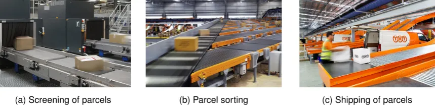
[image:10.595.84.515.179.286.2]

(11)

[image:11.595.85.515.37.143.2]

(a) Screening of parcels (b) Parcel sorting (c) Shipping of parcels

Figure 1.4: Example of parcel and postal systems

business (Vanderlande Industries, 2014). Therefore, for this market segment, as well as for the oth-ers, Vanderlande’s systems are becoming more complex due to more advanced technologies, higher throughput and larger utilization.

1.1.4 Customer services

Vanderlande offers a wide range of services to their customers. They can take care of preventive and corrective maintenance in different degrees. Site-based maintenance is possible as well as assistance via hotlines and help desks. Furthermore, Vanderlande can take over spare part management. In addition, the company can provide training about maintenance, equipment usage and safety. Moreover, life-cycle plans, logistics consultancy and process monitoring are services offered by Vanderlande as well. Finally, customers have the option to actively take part in the design process of their system by becoming a business partner (Vanderlande Industries, 2015b). All these customer services can be provided via custom made contracts.

1.2 Problem motivation

Downtime of a system is expensive for the customers of Vanderlande. For example, suppose the baggage handling system at a large airport breaks down. This has tedious and costly consequences such as passengers who are getting their luggage late. Therefore, availability of a system is an important key performance indicator during the design phase of a material handling system. Currently, each market segment within Vanderlande uses its own methods to calculate the availability of a system in the design phase. Moreover, the major part of the projects is done without a detailed availability study. In addition, even if a calculation is done, the calculated availability is often inaccurate, mostly resulting in a higher availability than the measured availability when the system is installed and operational at the customer. Since there is no standardized model, calculations can differ between market segments and even among projects in the same segment. In addition, service contracts are requested more and more by the customers of Vanderlande. Therefore, knowledge of expected failure behaviour and availability of the systems are crucial in order to calculate the expected service costs in an accurate way. Performing an availability study during the design phase can provide this knowledge. Finally, the availability calculations are done manually. All this gives rise to develop a standardized model that calculates the availability in a fast and accurate way.

(12)

1.2.1 Definition of availability

There are several ways to define availability, each definition with a slightly different interpretation. For example, Rausand & Hoyland (2004) define availability (according to the BS4778 quality vocabulary) as ’the ability of an item (under combined aspects of its reliability, maintainability and maintenance support) to perform its required function at a stated instant of time or over a stated period of time.’ This is a precise and complete theoretical definition. Vanderlande, however, uses a more practical definition as described by the European Federation of Materials Handling (1989):

’availability is the probability of finding a system at a given time in an operable condition.’

The complement of availability is unavailability which can be divided in two parts: operational and tech-nical unavailability. The first consists of downtime due to improper use of the system. For example, failures due to transport of products that are outside the allowed product dimensions fall within opera-tional downtime. Technical unavailability includes downtime due to technical failures such as worn out parts or software bugs. Vanderlande is only responsible for the technical availability of the system. It is the customer’s responsibility to use the system in the right way and the customer is therefore ac-countable for operational availability. Vanderlande and the customer together agree on the nature of the failure. This can partially be done in advance by making a list of possible failures and their nature. If not listed failures happen, Vanderlande and its customer will agree if it is a technical or operational failure.

To come back to Vanderlande’s definition of availability, it is not exactly clear what is meant by’an oper-able condition’. We define, using the definition of Vlasblom (2009), a system to be in operoper-able condition when the system can meet the throughput of baggage, parcels or materials, where Vanderlande and its customer agreed on. To be a bit more precise, we define technical unavailability as follows:

a system is unavailable when due to technical failure the system can not meet the throughput where Vanderlande and its customer have agreed on’ (Vlasblom, 2009).

With throughput we mean the required hourly peak flow of material handling units. For baggage han-dling, the throughput will be in terms of baggages per hour, whereas this is parcels per hour for the parcel & postal section. For warehouse automation, this can be for example pallets or cases per hour. To keep our model simple, we will focus on average availability over a long-term. However, Vanderlande will be penalized if the technical availability is below the agreed threshold. Therefore we prefer a model that can compute the availability for a specific time interval as well.

1.3 Research objective & questions

As discussed in the previous section, the aim of the study is to develop a standardized model for the technical availability calculation. Furthermore, we want to know how we can encourage people working at Vanderlande to make use of this model. We therefore formulate the following research objective:

Research towards a usable standardized model for calculating technical avaibility of automated material handling systems during the design phase.

(13)

1. Which models are suitable for calculating technical availability and what parameters are needed for it?

For this first question we study the literature and we interview several people within Vanderlande who are involved with the availability calculation. We describe the factors that significantly influence the system’s technical availability. Furthermore, we describe several methods to calculate availability and discuss their advantages as well as their disadvantages.

2. How is the current situation regarding availability calculations?

To answer the second research question we first study how the availability calculation is used within Vanderlande. Furthermore, we describe what model Vanderlande uses for each market segment. Third, we discuss the strengths and weaknesses of the currently used methods. Finally, we explain how Vanderlande measures availability of operational systems.

3. What is the most appropriate modeling approach for availability calculation for Vanderlande? Regarding the third question, to know what modeling approach is most suitable, we first need to know Vanderlande’s requirements for availability calculation. Next, we can weigh the alternatives and select the best modeling approach.

4. How can the chosen approach be applied at Vanderlande in order to develop the model? 5. How can the model be tested and validated?

By describing our availability model we answer the fourth and research question. We explain the input parameters we use and describe the calculation method. Finally, we discuss the testing and validation of our prototype model.

In the next section we describe the scope of our research.

1.4 Scope

In this section we discuss the scope of our research, because time for this research is limited. We describe which aspects we take into account and which are excluded from the research. Currently, Vanderlande calculates availability based on equipment. Using formulas for serial and parallel structures availability on higher levels is calculated. We base our model on the equipment level as well, because Vanderlande keeps track of the status of their equipment and thus availability data on equipment level is available within Vanderlande. Next, we do not focus on collecting input data. Collecting input data is not straightforward and will require too much time. However, we describe what input parameters are needed to take into account in the next chapter. We assume that spare parts are always available. Furthermore, because of the limited time available we do not take into account the maintenance policy.

Finally, the input data is outdated. Many of the component availability figures are not updated for years and it is not precisely known how these figures are obtained.

The remaining section of this chapter describes the methodology used to answer the stated problem definition and research questions and outlines briefly the content of the rest of the report.

1.5 Methodology and structure of the report

(14)

company. The main steps are identification of problems, analysis of the core problem, designing solu-tions, implementation of the chosen solution and evaluation of the results.

(15)

Chapter 2 Theoretical framework

In this chapter we answer our first research question: which models are suitable for calculating tech-nical availability and what parameters are needed for it? We outline the relevant literature regarding availability of a system. We start with discussing factors that influence the system availability in Section 2.1. Next, we describe four main models to model and calculate the availability. We end this chapter with a description of the component importance in Section 2.3.

2.1 Factors influencing system availability

This section discusses two main areas that have impact on system availability. The first area is the avail-ability of the individual components. The higher the components’ availavail-ability, the higher the availavail-ability of the system (Kuo & Wan, 2007). Second, the structure of the system has large impact on availability as well. (Kuo & Wan, 2007). We discuss the influence of component availability on system availability in Section 2.1.1 and the influence of the structure of the system in Section 2.1.2.

2.1.1 Component availability

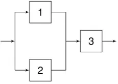
Component availability is an important determinant of system availability. In general, enhancing com-ponent availability comes with an increase in costs. Furthermore, not all comcom-ponents are of equal importance. For example, consider a system with three components. The first two parts are in paral-lel, whereas the third component is in series with the parallel structure. Figure 2.1 shows this system. Suppose all three components have equal availability. Enhancing the availability of the third component will have a larger impact than improving the availability of one of the other two components. To reach a required system availability it is important to compute the optimal availability of each component that minimizes the total cost (Mettas, 2000). There are several methods to solve this optimization problem. However, we will not discuss them here since this is out of our project scope. Nevertheless, identifying critical components can be useful during the design phase of a system. Section 2.3 describes how to calculate the importance of a component.

(16)

3 1

[image:16.595.240.356.35.117.2]

2

Figure 2.1: Example system

Ai =

M T T Fi

M T T Fi+M T T Ri

, (2.1)

whereAi is the availability of componentiandM T T Fi andM T T Ri are its mean time to failure and mean time to repair.

The mean time to failure is closely related to the quality and the load of the component The mean time to repair is mainly dependent on the nature of the failure, spare part logistics (Mettas, 2000), manpower for repair and its (corrective and preventive) maintenance policies (Topuz, 2009).

2.1.2 System structure

With respect to the structure of the system there are two aspects that have an impact on the system availability. The level of redundancy is important. With redundancy we mean components that are in parallel. The strongest level of redundancy is a pure parallel structure for which only one of the components needs to work. Lower levels of redundancy are structures for which only some of the components need to work. For example, if multiple components are placed in series, the system is down if one of the components fails. In contrast, for a parallel structure only one of the components needs to work to have a working system. The second aspect enhancing the system availability is reassignment of interchangeable components (Kuo & Prasad, 2000).

2.2 Availability calculation models

In this section we describe four methods to model system availability which can be found in literature. First we discuss the failure tree analysis method, followed by a description of the reliability block di-agram method. Next, we give an explanation of how Markov models can be applied to compute the availability of a system. We end this section with a description of simulation techniques to calculate system availability.

2.2.1 Failure tree analysis

(17)

TOP event

BE1 BE2 BE3

(a) OR gate

TOP event

BE1 BE2 BE3

(b) AND gate

TOP event

BE1 BE2 BE3

k/n

[image:17.595.102.469.129.308.2]

(c)kout ofngate

Figure 2.2: Failure tree gate representations

Top event

BE1 IE1

BE2 BE3

IE2

BE4 BE5 BE6

2/3

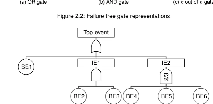
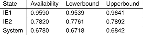
Figure 2.3: Fault tree example (Rausand & Hoyland, 2004)

required in a parallel structure. Figure 2.2 show the graphical representation of the OR gate, AND gate, andkout ofngate, respectively.

Several layers can be added to the fault tree until the desired level of detail is achieved. Figure 2.3 shows an example of a fault tree.

The fault tree can be analysed qualitatively or quantitatively. Since in this research we develop a quan-titative model we only discuss the quanquan-titative analysis. We use the approach described by Rausand & Hoyland (2004).

First we define variables describing the state of the basic events. These are the events on the lowest level of the tree:

Yi(t) =

  

1 basic eventioccurs at timet

0 otherwise.

(2.2)

The probability that basic eventi occurs at timet is denoted byqi(t), i.e. qi(t) = P(Yi(t) = 1). This probability can be seen as the unreliability of basic eventi. Letnrepresent the number of basic events in the fault tree. The state variables can be represented by a state vectorY(t) = (Y1(t), Y2(t), . . . Yn(t)). Next, the state of the TOP event is denoted by:

ψ(Y(t)) =

  

1 top event occurs at timet

0 otherwise.

(2.3)

Q0(t)is the probability that the TOP event occurs at timet, i.e. Q0(t) =P(ψ(Yi(t)) = 1). Thus,Q0(t)

represents the unreliability of the system.

(18)

ψ(Y(t)) =

n

Y

i=1

Yi(t) (2.4)

Q0(t) =

n

Y

i=1

qi(t). (2.5)

Serial components can be modelled with an OR gate. The state of the top event is given by equation 2.6. Assuming independent events, equation 2.7 shows formula for the unreliability of a serial struc-ture:

ψ(Y(t)) = 1−

n

Y

i=1

(1−Yi(t)) (2.6)

Q0(t) = 1−

n

Y

i=1

(1−qi(t)). (2.7)

Third,kout ofnstructures can be modelled with a special AND gate. If the components are identical, we can compute the unreliability using the binomial distribution (Rausand & Hoyland, 2004):

ψ(Y(t)) =

  

1 Pn

i=1Yi(t)≥k

0 Pn

i=1Yi(t)< k.

(2.8)

Q0(t) =

_n

y

n X

y=k

q(t)y(1−q(t))n−y. (2.9)

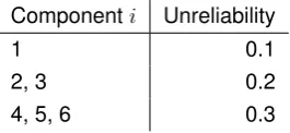
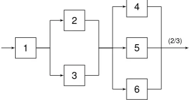
Consider the example shown by Figure 2.3. Suppose the components have unreliabilities as shown by Table 2.1. Furthermore, assume the components are independent and that the components 4, 5 and 6 are identical. We start with calculating the unreliability of the first intermediate event (IE1). This event occurs if both components 2 and 3 are not working. They are in parallel and we use the formula for parallel structures. Intermediate event 2 (IE2) is a 2 out of 3 structure. Since the components are identical we can use Equation 2.8:

QIE1(t) = 3

Y

i=2

qi(t) = 0.22= 0.04. (2.10)

QIE2(t) =

₃

y

3 X

y=2

q(t)y(1−q(t))n−y = 3·0.32·0.7 + 0.33= 0.216. (2.11)

Now we can compute the unreliability of the system. Basic event 1 and the two intermediate events are connected with OR gate, i.e. they are in series. Hence, we use the formula for a series structure:

Q0(t) = 1− 3

Y

i=1

(1−qi(t)) = 1−(1−0.1)(1−0.04)(1−0.216) = 0.3226. (2.12)

Calculating exact system (un)reliability can be time-consuming. Therefore we describe an approxima-tion method according to Rausand & Hoyland (2004). The approximaapproxima-tion uses minimal cut sets. The definition of a minimal cut set is, according to Rausand & Hoyland (2004):

(19)

Componenti Unreliability

1 0.1

2, 3 0.2

[image:19.595.232.365.36.97.2]

4, 5, 6 0.3

Table 2.1: Component availability of example system Top event

[image:19.595.139.457.132.236.2]

1 2,3 4,5 4,6 5,6

Figure 2.4: Fault tree showing minimal cuts

Generally, a minimal cut set has a parallel structure. Thus, a minimal cut set occurs if all its basic events occur. LetKdenote the number of minimal cut sets of the system. Note that the same basic event can be in multiple minimal cut sets. LetQˇj(t)denote the probability that minimal cut set Kj occurs. If all basic events occur independent of each other, then this probability is given by

ˇ

Qj(t) =

Y

i∈Kj

qi(t). (2.13)

A system can be modelled with its minimal cuts sets placed in series. The TOP event, system failure, occurs if at least one of the minimal cut sets occurs. Figure 2.4 shows the fault tree with minimal cuts of the example showed by Figure 2.3. Table 2.2 shows the unreliabilities of the minimal cut sets. There are structured methods to find the minimal cuts of a system (Rausand & Hoyland, 2004).

If all minimal cuts are independent of each other, than the system failure is given by

Q0(t) = 1−

k

Y

j=1

(1−Qˇj(t)). (2.14)

However, since the same basic event can be in multiple minimal cut sets the minimal cut sets are not always independent of each other. As can be seen in Figure 2.4, component 4, 5 and 6 are in two minimal cut sets. Therefore, the minimal cut sets are not independent. If the minimal cut sets are dependent of each other, they are positive correlated. A system with serial components that are positive correlated is more reliable than a system with independent components (Rausand & Hoyland, 2004), see Equation 2.15. Moreover, if the components of a system are highly reliable we can approximate the system unreliability as if it consists of independent multiple cut sets, as shown by Equation 2.16 (Rausand & Hoyland, 2004):

Minimal cut set Components UnreliabilityQˇj(t)

1 1 0.1

2 2,3 0.04

3 4,5 0.09

4 4,6 0.09

5 5,6 0.09

[image:19.595.181.414.690.782.2]

(20)

1

2

3

4

5

6

[image:20.595.200.395.40.143.2]

(2/3)

Figure 2.5: Reliability block diagram example

Q0(t)≤1−

k

Y

j=1

(1−Qˇj(t)) (2.15)

Q0(t)≈1−

k

Y

j=1

(1−Qˇj(t)). (2.16)

According to Rausand & Hoyland (2004), we need to be careful with this approximation if at least one of the unreliabilitiesqi’s is 0.01 or larger.

To come back to the example, since the minimal cut sets are dependent and not highly reliable, we can only compute an upper bound on the unreliability of the system:

Q0(t)≤1− 5

Y

j=1

(1−Qˇj(t)) = 1−(1−0.1)(1−0.04)(1−0.09)3= 0.3489. (2.17)

Since we already know that the exact unreliability is 0.3226, this is indeed a valid upper bound.

2.2.2 Reliability block diagram

The second model we discuss is modelling the system using a reliability block diagram (RBD). Figure 2.5 shows an example of a RBD. A reliability block diagram describes the function of the system. If a system consists of more than one function, a RBD is needed for each function. A system is represented by a network of basic elements using serial and parallel structures. In contrast to the fault tree which calculates the probability of system failure, the RBD method computes the probability that the system is functioning. This method is suitable for systems of non-repairable components and for systems in which the order of failures does not matter. However, there are extensions that deal with repairable and order-sensitive failures (Rausand & Hoyland, 2004). It is possible to convert a fault tree to a RBD and vice versa. However, sometimes it is difficult to do so. If there are shared components or if the system is large or complex, then it is generally hard to compute or convert a fault tree to a RBD.

2.2.3 Markov models

In this section we describe how Markov models can be used to model availability. But first, let us briefly explain what Markov models are. Suppose for each indext(e.g. timet) there is a random variableX(t)

(Ross, 2007). The state of the process attisX(t). The indextoften represent time. For example,X(t)

(21)

is called a Markov chain (Ross, 2007). Equation 2.18 shows the mathematical definition of a Markov chain. The main characteristic of a Markov chain is the memoryless property: a transition to a future state is dependent only on the current state and is independent on any of the past states.

P{Xn+1=j|Xn =i, Xn−1=in−1, . . . , X1=i1, X0=i0}=P{Xn+1=j|Xn=i}=Pij ∀i0, i1, . . . , in−1, i, j,andn≥0

(2.18)

If failure and repair times are exponentially distributed, automated material handling systems can be modelled as a Markov chain (Iyer et al., 2009). Each state can be seen as a combination of functioning and failed components. The transition to a future state represents the repair or failure of a single component. Since it does not matter how the system got into the current state, the probability of each transition is independent of the past states, but dependent on the current state. Therefore, the system can be modelled as a Markov chain.

Consider the example shown by Figure 2.5. One of the states is the situation in which all components are functioning. As a result, the system will be up. On the other hand, the state representing all components are functioning except component 1 indicates that the system will be down. For component 1 there are two states possible. For the parallel structure consisting of component 2 and 3, there are three possible states. Both components can work or can be in failure, or one of them can work. Since the two components are identical it does not matter which of them is in failure for this state. Likewise, the parallel structure consisting of components 4, 5 and 6 have four possible states. In total there are

2·3·4 = 24possible states. Only four states result in a working system. The large number of possible states shows a major disadvantage of this modelling technique. If the number of components increases, the number of states will increase exponentially. This is called the state space explosion problem (Ross, 2007). Although we can split up the system into multiple subsystems, computing the system availability will be time consuming.

2.2.4 Simulation

Simulation techniques can be used when it is difficult to use one of the previous discussed methods. Below we discuss a simple way to simulate the system and compute the availability.

Simple continuous time simulation

The simplest time simulation used for availability calculation are based on Monte Carlo simulation. Monte Carlo simulation can be defined as a scheme which makes use of random numbers to solve stochastic or deterministic problems (Law, 2007). This scheme is repeated many times and the occur-rences number of specific events is counted (Takeshi, 2013). Monte Carlo simulation is a technique without time dimension. However, failure and repair rates are time-based. Therefore, a time dimension is often added to the simulation. It is broadly used for complex systems (Lu et al., 2012) that are not analytically manageable. For example, simple time simulations can easily deal withk out ofn struc-tures, redundancies, repair and maintenance (Takeshi, 2013). The simulation can be seen as a series of real experiments (Takeshi, 2013). Statistical techniques are used to estimate the mean and confi-dence intervals. A weak aspect of this method is that its computation time can be large. For systems with highly reliable components the sample size needs to be large to provide reliable estimates (Korver, 1994).

(22)

State Availability Lowerbound Upperbound

IE1 0.9590 0.9539 0.9641

IE2 0.7820 0.7761 0.7892

[image:22.595.180.421.37.96.2]

System 0.6780 0.6718 0.6842

Table 2.3: Results simple continuous time simulation (1000 replications) for example system

allow that our interval width deviates at most one percent of our approximation. We use the sequential method (Law, 2007) to determine the required number of replications. We need 1000 replications. For each replication, we draw a random number [0,1] from the Uniform [0,1] distribution for each component. If this random number is lower than the failure probability, we consider this component as working; otherwise a failure occurred during this time interval. If a failure occurred during the previous time interval, we draw a second uniform distributed random number [0,1]. If this random number is higher thane−µ∆twithµis 1 divided by the mean time to repair, we consider this segment as been repaired. Once we know the status of the components, we can compute the status of the system. The system availability is the average of the system status of all replications. Furthermore, we compute the 95% confidence interval. Table 2.3 shows the availability and interval of the (sub)system(s).

2.3 Component importance

It is clear that some components have more impact on system availability than others (Rausand & Hoyland, 2004). In this section we discuss a method to measure the component importance. The im-portance of a component is related to the function(s) it has within the system. A component that is used in two system functions could be highly important for one function, but less important for the other function. There are several ways to measure component importance. Since this research focusses on the design phase of a system, we look for a method to identify bottlenecks or weak points of the system. Once the weak elements of the system are identified, system designers can decide whether improve-ment of these eleimprove-ments is desired. To identify the weak components within a system we calculate the improvement potential of each component. This variable states how much the availability of the system will increase if the component is replaced by a perfect one (Rausand & Hoyland, 2004). With a perfect element we mean a element that cannot fail. Hence, the component is always available. Consider a system with multiple components. We denote the probability of a working componentiat timetbypi(t) and the probability of a working system byh(p(t)). Here, p(t) is the vector of the individual compo-nents’ probability. The improvement potential of an elementiat timetis given by (Rausand & Hoyland, 2004):

IIP(i|t) =h(1i,p(t))−h(p(t)) ∀i= 1, . . . , n (2.19)

In practice, it might not be possible to replace a component with a perfect one. We can then use the same equation, but we use the highest possible failure probability that is still realistic. The obtained potential is called credible improvement potential (Rausand & Hoyland, 2004).

Once the improvement potential of all the components are computed, we can rank them to identify the bottlenecks of the system with respect to availability. Availability improvement of the component with the highest improvement potential will result in the largest increase in system availability (Zhang, 2014). Furthermore, we can check whether there are differences between availabilities of subsystems. Unfortunately, the importance of a component does not provide information on how the element could be improved.

(23)

Component A1 AIE1 AIE2 As Improvement potential

1 1.0 0.96 0.784 0.7526 0.0753

2, 3 0.9 1.0 0.784 0.7056 0.0282

4, 5, 6 0.9 0.96 0.91 0.7862 0.1089

Table 2.4: Improvement potentials of example system

we replace component 1 by a perfect component, the unavailability of component 1 becomes zero, but the rest of the system remains the same. The new unreliability is

Q0(t) = 1− 3

Y

i=1

(1−qi(t)) = 1−(1−0)(1−0.04)(1−0.216) = 0.2766. (2.20)

IIP(i|t) =h(11,p(t))−h(p(t)) = (1−0.2766)−(1−0.3266) = 0.0753. (2.21)

We can calculate the improvement potential of the other components in the same way. Table 2.4 shows the improvement potential of each component. As can be seen, component 4, 5 and 6 have the highest improvement potential. If we want to change one component, it would be one of these. This will result in the largest increase of system availability. This is no surprise, because the availability of these components is relatively low and at least two of them need to work. In general, component improvement costs money. Therefore, we have to make a trade-off between availability improvement and costs.

2.4 Summary

In this chapter we discussed the following points:

• System availability is determined bycomponent availabilityand thestructure of the system.

• We have discussed five availability calculation models. With fault trees and reliability block diagramswe model the system by decomposing it into building blocks. With formulas for serial, parallel and k-out-of-n structures we can calculate system availability. For simple systems we can calculate this exactly; for more complex systems we need approximations. Markov models consider the system as a whole and its possible states. It can be used if the failure and repair times are exponentially distributed. This method is only suitable for small systems, because the number of system states rapidly increases for larger systems.

If the system is too large or too complex to calculate (or accurately approximate) the system availability, we can use simulation techniques. Simple continuous time simulationmakes use of random numbers to simulate the state of each component. These statuses are used to obtain the system status. The simulation is replicated many times. The system availability is the average system status. If we need more details, we can simulate the system in more detail usingdiscrete event simulation.

(24)

(25)

Chapter 3 Current situation

In this chapter we analyse the current situation regarding availability calculation and measurement. By doing so, we answer our second research question. We start with a discussion of the usage of availability calculations within Vanderlande in Section 3.1 and we briefly explain the design process in Section 3.2 and the two availability related industry standards used by Vanderlande. Next, we describe the three availability calculation methods that Vanderlande uses in Section 3.4. Then, in Section 3.5 we describe how availability is measured for operational systems. We end this chapter with a discussion of the strengths and weaknesses of the current availability calculation methods in Section 3.6.

3.1 Usage of availability calculations

Availability calculations are made based on customer’s request. However, customers are often satisfied with an availability figure without calculation. As a result, Vanderlande has done availability studies for only a small fraction of their projects. Consequently, there is currently little knowledge on availability and failure behaviour of the system during sale and design phase. This is not necessarily a problem. However, the agreed availability can be defined in a service contract which is requested more and more by the customers. It happens regularly that an agreed availability figure is higher than the measured availability once it is operational at the customer.

3.2 Sales and design process

(26)

3.3 Industry standards: FEM & VDI

Within the automated material handling industry there are two industry standards referenced regularly. Since these standards are important in the eye of Vanderlande and its customers, we discuss them here as well. The first standard is called FEM 9.222 and is developed by the European federation of handling (FEM). The standard gives a definition of availability together with formulas how to calculate availability (European Federation of Materials Handling, 1989). FEM implicitly use the fault tree method and the formulas for a serial and parallel structure are the same as discussed in Chapter 2. However, they do not mention how to calculate the availability of ak-out-of-nstructure. The other standard is called VDI 3649 and is developed by the association of German engineers (VDI). The standard gives a definition for availability (Verein Deutscher Ingenieure, n.d.). Like the FEM standard they implicitly assume a fault tree decomposition of the system. Again the formulas for a serial and parallel structure are the same as discussed in Chapter 2. Furthermore, they give an example ofk-out-of-nsystem. Although they give some formulas to calculate the availability of the example system, they do not provide generalized formulas that do apply for generalk-out-of-nstructures.

3.4 Vanderlande’s availability calculation

Vanderlande uses fault tree analysis (FTA) to calculate the technical availability of designed systems, regardless of their corresponding market segment. The failure tree analysis method is already explained in Section 2.2.1. The lowest level that Vanderlande considers is the equipment level. Examples of components on this level are normal and curved conveyor belts, sorters, and screening machines. The research and development department is concerned with providing the input data. For each component on equipment level, they compute the mean time between failure (MTBF) and the mean downtime (MDT). The department obtains the data by doing a short time study or retrieves the data from the equipment supplier. Below we explain the three calculation methods that are used by Vanderlande. The system’s layout and the material flow diagram are used to make the fault tree. This is done manually. Next, the fault tree structure and its availabilities are put in Excel. Formulas for serial and parallel structures are added in order to calculate the availability of the system. These formulas are based on the industry standards FEM 9.222 and VDI 3649. Below we explain the three methods that are used to calculate the availability within Vanderlande.

3.4.1 Method 1

This method is mainly used for smaller baggage handling projects. However, it is sometimes used for other types of projects as well. As described above, the availability calculation starts with the con-struction of a failure tree. For the first method, this tree is static using serial, parallel ork-out-of-n (k

(27)

1 2 3 4 5 6 (2/3)

(a) Reliability block diagram

Top event

1 IE1

2 3

IE2

4 5 6

2/3

[image:27.595.95.474.40.194.2]

(b) Fault tree

Figure 3.1: Example of a system consisting of serial and parallel structures

Componenti Availability

1 0.9

2, 3 0.8

4, 5, 6 0.7

Table 3.1: Component availability of example system

¯

As≈1− n

Y

i=1

(1−A¯i) (3.1)

¯

As≈ n

Y

i=1 ¯

Ai (3.2)

¯

As≈

n n−k+ 1

¯

Ai n−k+1

, (3.3)

whereA¯s represents the unavailability of the (sub)system and A¯i the unavailability of the underlying componenti. For ak-out-of-nstructuren−k+ 1components need to fail to have a failed (sub)system. The formulas for a serial or parallel structure are similar to the formulas discussed in Chapter 2. How-ever, the formula for akout ofnstructure is different. Moreover, the given formula in (3.3) is not mathe-matically correct since it is possible to get an (un)availability larger than 1. For example, consider a sys-tem where 18 out of 20 identical components need to work to have a working syssys-tem and suppose the availability of each component is 0.9. Then the unavailabilityA¯s≈ ₂₀₋20₁₈₊₁A¯i

20−18+1 = 20₃

0.13_≈₁_.₁₄

which cannot be true. However, Vanderlande uses this formula because it is a simple approximation. It aims at calculating the probability of the minimal number of failed elements such that the system is down. They assume that the probability that more than this minimal number of elements fail is negligible. We discuss this issue in more detail in Section 3.6.

To come back to the example showed by Figure 3.1, suppose the following component availabilities as showed by Table 3.1.

[image:27.595.234.364.246.307.2]

(28)

Componenti Capacity

1, 2, 3 120

4, 5, 6 60

Table 3.2: Capacity of example system

1 2 3 4 5 6 120/120 60/120 60/120 40/60 40/60 40/60 (2/3)

Figure 3.2: Example with flow through the components

¯

AIE2≈

₃

2

¯

A24= 0.3 2

= 0.0810 (3.4)

¯

AIE1≈

₂

2

¯

A2₂≈

₂

2

0.22= 0.0400 (3.5)

¯

AT E = 1−(1−A¯1)(1−A¯IE1)(1−A¯IE2)

= 1−0.9·0.96·0.919≈0.2060 (3.6)

AS = 1−A¯T E≈0.7940, (3.7)

where the availability of the system is given byAS, A¯T E stands for the unavailability of the top event andA¯IE1andA¯IE2represents the unavailability of the intermediate events.

3.4.2 Method 2

The second method is the most simple one of the three methods that Vanderlande uses. The method is called the SPA (serial parallel availability). It was originally developed for large baggage handling systems, but is used for other projects as well. The calculation of a series structure is the same as for the previous method.

This method calculates the availability instead of the unavailability. Furthermore, the calculation of the previous method does not take into account capacities of the elements whereas the second method does take this into account. Consider again the example shown by Figure 3.1 and suppose the required throughput is 120 units per hour. Furthermore, suppose the elements have capacities as shown by ??.

We assume that the flow through the parallel elements is equally spread over the elements. Figure 3.2 shows the block diagram with the corresponding flow through the elements. Since the capacity of elements 2 and 3 is 120, only one of the two elements need to work which was the case in the previous example as well. Furthermore, two elements of the elements 4, 5 and 6 can handle the required throughput, so two out of three elements need to work. This is again in line with the previous example.

(29)

As≈ n

Y

i=1

Ai (3.8)

As= n

X

i=1

wiAi (3.9)

withwi=

Ci

Pn

j=1Cj

,

wherewiis the weight factor for elementiwhich is the capacity of elementidivided by the total capacity for the parallel structure. As can be seen, it is simple to calculate the availability of a parallel structure. One can imagine that simple formulas are necessary to obtain availabilities of complex systems in a short period of time. Moreover, during the sales phase the design of the system can change multiple times. To recalculate te availability in a fast way, a simple calculation method is desired. We discuss the consequences of this approximation in Section 3.6.

Again consider the system example depicted by Figure 3.2. The availability of the second parallel structure is equal to the availability of element 4, 5 and 6 since these elements have equal capacity and availability. The same reasoning applies for the first parallel structure. The system’s availability can be calculated as follows:

AS =A1AIE1AIE2= 0.9·0.8·0.7 = 0.5040 (3.10)

withAIE1=w2A2+w3A3= 2· 120

2400.8 = 0.8

andAIE2=w4A4+w5A5+w6A6= 3· 60

1800.7 = 0.7.

3.4.3 Method 3

The last method is the most complex method and is mainly used for parcel & postal projects. As for the previous method, this method takes capacity into account though the calculation for a parallel structure is different. Since parallel elements are often not used at their maximum capacity there is spare capacity which can be used when one or more parallel elements fail. From this perspective, there is no clear

k-out-of-nstructure, but we rather look at the capacity loss when an element is unavailable which might be only a small fraction of the required throughput.

The following formulas are used to calculate the unavailability of a serial and parallel structure:

As≈ n

Y

i=1

Ai (3.11)

As= 1−

X

∀ω∈Ω ¯

AωLω (3.12)

withA¯ω=

Y

∀i∈ω

¯

Ai

Y

∀j /∈ω

Aj

andLω= max{0; 1−

X

∀i /∈ω

pi},

where Ω is the set of all possible combinations of parallel components, A¯ω the unavailability of the combinationω∈Ω,Lωrepresents the loss of capacity due to unavailability ofωandpiis the fraction of required flow that elementican handle.

(30)

1

2

3

4

5

6 120

0

120

40

(2/3)

Figure 3.3: Example with flow through the components - component 2 is down

component 2 is down. Figure 3.3 shows this situation. Since component 3 has a capacity of 120 the system can still handle the required flow of 120 and the parallel structure is still available. Only if component 2 and 3 are both down the system will be down. Thus, method 3 takes into account the consequences of lost capacity due to the failure of components. For each combination of working and failed componentsω we calculate the loss of capacity Lω and the unavailability of this combination. The unavailability of the parallel structure is then the sum of the unavailability multiplied by its loss of capacity.

For parallel structures (only one of all components need to work) formula 3.12 is equal to Rausand’s method of parallel structures. However, for k-out-of-n-structures it overestimates the availability. We discuss this more detailed in section 3.6.

We return to the example system depicted in Figure 3.2. To calculate the availability of intermediate event 2 (IE2), we first need to list all possible combinations of parallel components and the fraction of flow that each element can handle:

ΩIE2= {},{4},{5},{6},{4,5},{4,6},{5,6},{4,5,6}

(3.13)

p4=p5=p6= 60

120 = 0.5. (3.14)

Next, we calculate the unavailability of each combination and its corresponding loss of capacity:

¯

A{}= 0.73= 0.3430 (3.15)

¯

A{i}= 0.3·0.72= 0.1470 i= 4,5,6 (3.16)

¯

A{i,j}= 0.32·0.7 = 0.0630 {i, j}={4,5},{4,6},{5,6} (3.17)

¯

A_{4,5,6}= 0.33= 0.0270 (3.18)

L_{}=max{0; 1−0.5−0.5−0.5}= 0 (3.19)

L{i}= max{0; 1−0.5−0.5}= 0 i= 4,5,6 (3.20)

L{i,j}= max{0; 1−0.5}= 0.5 {i, j}={4,5},{4,6},{5,6} (3.21)

L{4,5,6}= max{0; 1}= 1. (3.22)

Now we can compute the availability of the parallel structure IE2:

AIE2= 1−A¯{}L{}−3 ¯A{4}L{4}−3 ¯A{4,5}L{4,5}−A¯{4,5,6}L{4,5,6}

= 1−0.3430·0−3·0.1470·0−3·0.0630·0.5−0.0270·1≈0.8785. (3.23)

(31)

ΩIE1= {},{2},{3},{2,3}

(3.24)

pi=

120

120 = 1.0 i= 2,3 (3.25)

¯

A{}= 0.82= 0.6400 (3.26)

¯

A{i}= 0.2·0.8 = 0.1600 i= 2,3 (3.27)

¯

A{2,3}= 0.22= 0.0400 (3.28)

L{}=max{0; 1−1−1}= 0 (3.29)

L{i}= max{0; 1−1}= 0 i= 2,3 (3.30)

L{2,3}= max{0; 1}= 1 (3.31)

AIE1= 1−A¯{}L{}−2 ¯A{2}L{2}−A¯{2,3}L{2,3}

= 1−.6400·0−2·0.1600·0−0.0400·1 = 0.9600. (3.32)

Then, the availability of the system is given by:

AS =A1AIE1AIE2= 0.9·0.96·0.8785≈0.7590. (3.33)

This system availability is lower than the availability using the first methods while the system is exactly the same. Furthermore, this method is more cumbersome than the previous methods. Moreover, the number of possible combinations of parallel elements can be very large a structure with more parallel components. We discuss this issue in more detail in Section 3.6.

Before we discuss the shortcomings of the used methods, we first describe the assumptions and the measurement method of Vanderlande.

3.4.4 Assumptions for availability estimation

Vanderlande assumes typically that equipment runs for 20 hours a day. Availability of screening ma-chines is not taken into account, because Vanderlande states that these mama-chines are not part of the scope of supply. Failures of scanners or manual coding station equipment, like computers, are not taken into account in the availability calculations, because Vanderlande states that failure of this equipment will not hamper the baggage flow. Besides these assumptions, Vanderlande has a list of exclusions which can be different between projects. There are operational assumptions such as the exclusion of malfunc-tions due to material clogging not caused by Vanderlande’s (sub)systems or equipment and failures due to products that are outside allowed parameters including weight and dimensions. Furthermore, inter-ruptions or delays caused by operators or unauthorised persons are excluded as well. There could be reasons to exclude non-operational things as well. For example, a common exclusion of Vanderlande is to exclude incipient failures that are detected and repaired without affecting the normal functioning of the system. Sometimes, downtime less than one minute is excluded, because Vanderlande states that such short downtime periods can be neglected in practice. Furthermore, availability of servers and associated controls is often not taken into account because Vanderlande states that their availability is extremely high compared to the availability of the other equipment and will have no significant effect on overall availability of a subsystem.

3.5 Availability measurement

(32)

that are placed in a serial or parallel configuration (Lassche, 2015). Larger systems can first be split up into areas that consist of one or multiple function blocks. The method states that this implies certain independency and therefore areas are connected in parallel. Function blocks are defined as parts of the system that serve the same function (Lassche, 2015). If one of the elements fail, the entire function block will fail. Therefore, a function block can be seen as serial elements. A failure can have a technical or operational cause. For each error, the probability that it is a technical or operational error is defined beforehand. If an error occurred causing a certain downtime, this downtime is assumed to be technical downtime for a fraction equal to the technical error probability. The remaining downtime is assumed to be operational downtime. Within a function block it can happen that failures overlap with each other. For example, a second failure occurs while the first failure is not yet repaired. During the overlapping errors, it might not be exactly clear if it is due to a technical or operational cause. Therefore, they use a weighted average to define which part is a technical downtime. Furthermore, minimum and maximum repair times are defined to compensate for operator caused delay repair time. Minimum repair time compensates for start-up time such as travel distance to the failed component. Maximum repair times are used for repair times that are longer than reasonable. For example, repair times might be unreasonably long if the operators are poorly trained. The formulas for serial and parallel structures are the same as the formulas of Method 3. However, they have added the possibility to add relative weights to the function blocks. This is done because some function blocks handle processes that are more critical than others (Lassche, 2015). Since this method is relatively new, there are no projects for which this method is implemented and an availability study was made using method 3.

3.6 Shortcomings of the current situation

In this section we explain the shortcomings of the three used methods for availability calculation within Vanderlande.

The measurement of availability, i.e. the availability calculation once the system is implemented, is different for each of the three calculation methods. This makes it difficult to compare the expected availability with the realized availability. Furthermore, all these methods indirectly assume that all com-ponents are independent of each other. However, it is questionable if this is a realistic assumption. If the failure probability is dependent on the load of the component, then components in a parallel struc-ture are dependent on each other. If one of the components fails, the load of the other components increases and hence the failure probability increases. In addition, there are two drawbacks of using fault trees. First, employees can interpret the system structure differently and translate the layout into different fault trees. This results in different availability calculations. Furthermore, manually translating the system into a fault tree and calculating the availability by hand (with the use of spreadsheets) takes a lot of time. Moreover, the quality of the fault tree depends on the time that is available for the avail-ability study. Next to that, none of the methods allows for multiple input types. For example, a customer wanting a new baggage handling system for their airport might require a specific througput for interna-tional and domestic check-in baggage and transfer baggage. The methods used by Vanderlande do not provide information how to calculate system availability with these three different input flows. Besides, Vanderlande states many assumptions and exclusions for their availability calculation. It is questionable if the calculation is still realistic, useful and reliable. Finally, the input data is outdated. Many of the component availability figures are not updated for years and it is not precisely known how these figures are obtained.

To summarize, we discussed the following general aspects:

1. Availability calculation during operationalization different from design phase calculation; 2. Independent components assumption;

(33)

4. Fault tree construction takes a long time; 5. Methods do not allow for multiple input types; 6. Many assumptions and exclusions;

7. Outdated input data.

Besides the general drawbacks of the methods, there are some drawbacks of each specific method which we will discuss below.

3.6.1 Method 1

This method does not take into account the capacities of the components. This can be a problem when capacities are not identical, because then it is difficult for parallel andkout ofnstructures to determine how many components need to work. Furthermore, as we have seen already in Section 3.4, using method 1 it is possible to get an (un)availability larger than 1. This is caused by the formula used for

k out ofnstructures, see Equation 3.34. First, this formula assumes that all components are equal, because there is no summation or product over indexi. Second, this formula ignores the probability that more thann−k+ 1components are not working. Vanderlande ignored this probability, because this probability is generally very small. However, the probability that n−k+ 1 identical components are not working is not correctly calculated. Equation 3.35 shows the correct formula. As can be seen, Vanderlande ignores the last part of the equation. This can results in (un)availabilities larger than 1.

¯

As≈

n n−k+ 1

¯

Ai n−k+1

, (3.34)

P(n−k+ 1not working) =

_n

n−k+ 1

¯

An−k+1Ak−1. (3.35)

3.6.2 Method 2

In contrast to the first method, method 2 is mathematically correct. However, there are issues with the formula for parallel structures (see Equation 3.36). System availability is considered as a capacity based weighted average of the component availabilities. This can be seen as the fraction of total capacity that is available. However, this ignores the required throughput of the structure. Generally, only a fraction of the total capacity of the structure is needed to reach the required throughput. Furthermore, this clearly underestimates the availability of a parallel structure. The power of a parallel structure is that only one (orkin case of akout ofnstructure) component needs to work.

As= n

X

i=1

wiAi (3.36)

withwi=

Ci

Pn

j=1Cj

.

3.6.3 Method 3

(34)

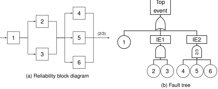
Ai Method 1 Method 2 Method 3 Exact method

AS 0.7940 0.5040 0.7590 0.6774

AIE1 0.9600 0.8000 0.9600 0.9600

[image:34.595.93.479.78.347.2]

AIE2 0.9190 0.7000 0.8785 0.7840

Table 3.3: Availability of example system

1

2

3

4a 4b

5

6

(2/3)

(a) Reliability block diagram

Top event

1 IE1

2 3

IE2

IE3

4a 4b

5 6

2/3

(b) Fault tree

Figure 3.4: Extended example system

However, according to our definition of availability defined in Chapter 1, the system will be unavailable if the required throughput cannot be met. Furthermore, the difference in k-out-of-n structure’s availability between method 3 and the exact approach can become larger when the component availabilities are not identical.

3.6.4 Comparison

Table 3.3 shows the availabilities of the (sub)systems for each method, together with the exact calcu-lation, which we discussed in the Chapter 2. For this small example, we can clearly see differences between the computed availabilities. For large and complex systems such as the systems that Van-derlande designs, the differences will be even larger. We can see that the availability of the parallel structure (IE1) of method 1 and 3 are in line with the exact calculation. Method 2 underestimates paral-lel structures, resulting in a lower availability for structure IE1. Method 2 underestimates the availability of thek out ofn structure (IE2) as well. In contrast, method 1 and 3 overestimate the availability of structure IE2. This results in an overestimation of the system availability as well. Method 2 gives an underestimation of the system availability.

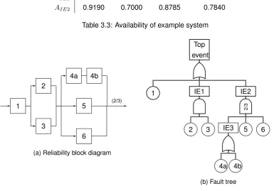
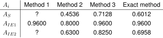
Consider again our example system, depicted in Figure 3.1a, but now component 4 is split into to components, 4a and 4b. The two components are in series and suppose that both components have availability of 0.7. Figure 3.4 shows this new situation. Table 3.4 shows the obtained availabilities of each method. As we can see, method 2 (3) still underestimates (overestimates), but now relatively more. For method 1, we cannot calculate the availability of thekout ofnstructure, because element 5 and 6 have an availability of 0.7, whereas component 4a and 4b together have an availability of0.72 _{= 0}_.₄₉_{. Since}

the formula forkout ofnstructure assumes identical components, we cannot evaluate the availability of this structure.

(35)

Ai Method 1 Method 2 Method 3 Exact method

AS ? 0.4536 0.7128 0.6012

AIE1 0.9600 0.8000 0.9600 0.9600

[image:35.595.165.430.123.185.2]

AIE2 ? 0.6300 0.8250 0.6958

Table 3.4: Availability of example 2 system

0.00 0.10 0.20 0.30 0.40 0.50 0.60 0.70 0.80 0.90 1.00 −0.20

−0.10 0.00 0.10 0.20 0.30 0.40 0.50 0.60 0.70 0.80 0.90 1.00

Component availability

System

a

v

ailability

Method 1 Method 2 Method 3 Exact method

[image:35.595.125.468.395.692.2]

(36)

...

1

2

3

4 5 6

...

(2/3)

[image:36.595.147.451.34.208.2]

(2/3)

Figure 3.6: Example system with62= 36components

We can see that method 1 results in negative system availability for small component availabilities. Furthermore, method 2 underestimates the system availability regardless the availability of the compo-nent. In contrast, method 3 overestimates system availability. Method 2 overestimates for component availabilities larger than 0.40. The graph shows that even for small systems, the differences between the methods are clear. Vanderlande typically has systems with highly reliable components. The differ-ence between the exact calculation and method 1 and 3 becomes smaller as the component availability comes close to 1. However, method 2 gives even for large component availabilities substantially lower system availability than calculated in the exact way.

The equipment that Vanderlande uses such as conveyor belts, sorters and screening machines, are generally highly reliable. Therefore, their availability is close to one. Most of the parts have availability above 99.5% and we can state that 98% is the minimal equipment availability. When we zoom in on availabilities close to one, method 1 and method 3 are almost equal to Rausand’s exact method. Figure 3.7a) shows this. However, the systems of Vanderlande have typically thousands of components. So suppose that each component of our example system actually consists of a subsystem with the same layout. Figure 3.6 shows this example. As can be seen, this system consists of six subsystems with six components each. Thus, we have 62 _{= 36} _{components in this system. Now assume that each}

component in the subsystems on its turn consists of a subsystem as well. Then there are 63 _{= 216}

components within the system. We can further expand this system into a system with6n components. As the number of components within the system increases, the deviation of each of Vanderlande’s methods from the exact method becomes larger. Figure 3.7 shows the system availability as a function of the component availability forn= 1,2,4,6.

Now we have seen how the current methods perform, we can move to the development of a new availability calculation model. In the next chapter we discuss the requirements for this model and we define four alternative calculation models. But first we summarize our findings regarding the current situation.

3.7 Summary

In this chapter we discussed the following points:

• Currently, Vanderlande has little knowledge on availability and failure behaviour of the system during sale and design phase.

• We discussed the sales and design process, from new lead to signed contract.

(37)

0 . 980 0 . 985 0 . 990 0 . 995 1 . 000

0.980 0.985 0.990 0.995 1.000

System

a

v

ailability

M1 M2 M3 Exact

(a)61_{= 6}_components

0 . 980 0 . 985 0 . 990 0 . 995 1 . 000

0.980 0.985 0.990 0.995 1.000

System

a

v

ailability

M1 M2 M3 Exact

(b)62_{= 36}_components

0 . 980 0 . 985 0 . 990 0 . 995 1 . 000

0.980 0.985 0.990 0.995 1.000

System

a

v

ailability

M1 M2 M3 Exact

(c)64_{= 1296}_components

0 . 980 0 . 985 0 . 990 0 . 995 1 . 000

0.980 0.985 0.990 0.995 1.000

System

a

v

ailability

M1 M2 M3 Exact

[image:37.595.96.508.184.630.2]

(d)66_{= 46656}_components

(38)

Series Parallel k-out-of-n

Method 1 A¯s≈1−Q n

i=1(1−A¯i) A¯s≈Q n

i=1A¯i A¯s≈ _n₋n_k₊₁

_¯

Ai n−k+1

Method 2

(SPA) As≈

Qn

i=1Ai

As=P n i=1wiAi withwi=PnCi

j=1Cj

see parallel

Method 3 As≈Q n i=1Ai

As= 1−P∀ω∈ΩA¯ωLω withA¯ω=Q_∀i∈ωA¯iQ_∀j /∈ωAj andLω= max{0; 1−P_∀_{i /}_∈_ωpi}

see parallel

Exact method

¯

As= 1− n

Q

i=1

(1−A¯i)

for independent components

¯

As= n

Q

i=1 ¯

Ai

for independent components

¯

As=Pn_y₌_k n_yA¯i y

(1−A¯i)n−y for independent and

[image:38.595.74.580.35.189.2]

identical components Table 3.5: Vanderlande’s three calculation methods versus exact method from literature

calculate the system availability are different (see Table 3.5).

Method 1 is mainly used for smaller baggage handling projects whereas method 2 was originally developed for large baggage handling systems. Method 3 is mainly used for parcel & postal projects and warehouse automation projects. For all three methods, Vanderlande has defined assumptions and exclusionsregarding the availability of the system. These can differ among projects.

• Last year, Vanderlande developed a new method to measure availabilityof installed systems. This method is similar to method 3.

Towards a standardized availability model for material handling systems

TOWARDS A

STANDARDIZED

AVAILABILITY MODEL

Management summary

Table of contents

Preface

Chapter 1

Introduction

1.1

Vanderlande Industries

1.1.1

Baggage handling

1.1.2

Warehouse automation

1.1.3

Parcel & postal

1.1.4

Customer services

1.2

Problem motivation

1.2.1

Definition of availability

1.3

Research objective & questions

1.4

Scope

1.5

Methodology and structure of the report

Chapter 2

Theoretical framework

2.1

Factors influencing system availability

2.1.1

Component availability

2.1.2

System structure

2.2

Availability calculation models

2.2.1

Failure tree analysis

2.2.2

Reliability block diagram

2.2.3

Markov models

2.2.4

Simulation

2.3

Component importance

2.4

Summary

Chapter 3

Current situation

3.1

Usage of availability calculations

3.2

Sales and design process

3.3

Industry standards: FEM & VDI

3.4

Vanderlande’s availability calculation

3.4.1

Method 1

3.4.2

Method 2

3.4.3

Method 3

3.4.4

Assumptions for availability estimation

3.5

Availability measurement

3.6

Shortcomings of the current situation

3.6.1

Method 1

3.6.2

Method 2

3.6.3

Method 3

3.6.4