Predicting the performance of business partners, using issue data of the iSense system : mapping a perception to data using machine learning

(1)

Predicting the performance of business partners, using issue data of the iSense system

Mapping a perception to data using machine learning

Master thesis

Dennis Muller

University of Twente supervisors: Maurice van Keulen & Bart Nieuwenhuizen

Nedap supervisor: Jaap Zaal

Faculty of Electrical Engineering, Mathematics and Computer Science University of Twente

(2)

Abstract

(3)

Preface

(4)

CONTENTS CONTENTS

List of Figures

1 An iSense system with gates at a store . . . 3

2 An iSense system that is overhead at a store, the system is attached to the roof instead of a gate . . . 3

3 The hierarchy of Nedap . . . 4

4 How the model is created and used to make predictions . . . 5

5 The CRISM-DM process . . . 6

6 The division of machine learning techniques and the algorithms . 15 7 A simple classification example . . . 16

8 A simple clustering example . . . 17

9 A simple association example . . . 19

10 Total amount of issues above the duration on the X-label . . . 29

11 Visualization of overfitting and underfitting . . . 44

12 An example how a MinMax-scalar scales the data . . . 46

13 A simple regression tree . . . 50

14 A simple gradient boosting regressor . . . 50

15 The regression tree with friedmans MSE as error function, the top two splits can be seen . . . 70

16 The regression tree with MAE as error function, the top two splits can be seen . . . 70

(8)

LIST OF TABLES LIST OF TABLES

List of Tables

1 Issue type with the statistics and category of each type . . . 25

2 Responsibility Matrix, responsibility against issue type with how much impact an issue type has . . . 27

3 Issue type with the statistics and category of each type . . . 37

4 Business partners ratings from questionnaire and interviews . . . . 39

5 An overview of all candidate features, these are repeated for local retailers and global retailers . . . 41

6 Accuracy percentages by different cases . . . 48

7 Accuracy percentages by different cases . . . 55

8 The different gradient boosting regressors and parameters . . . 56

9 The different regression trees and parameters . . . 57

10 The different error percentages of the different models, the columns show the iteration number and the rows show the error percentage per model . . . 57

11 The predicted rating of a business partner with the average per-ception of the interviewees . . . 64

(9)

1 INTRODUCTION

1 Introduction

(10)

1.1 Objectives 1 INTRODUCTION

Nedap does not install the systems themselves. Nedap has a global network of business partners, which install Nedap’s solutions at the retailers. Nedap is active in over 127 countries and each country has at least one business partner. Each business partner has its own region in which they are active and responsible for the systems. This is not only installation, but also servicing the retailers after in-stalling the systems to ensure maximum quality. The way this hierarchy works can be seen in figure 3 Importantly Nedap stores all data of these systems and create platforms for the retailers, business partners and themselves to see issues of the systems and allow for remote connections to solve them. This means that the business partners are directly responsible for ensuring that the systems are in-stalled correctly, issues that come up are resolved and configuration of the system is done correctly. The business partners are directly responsible for the quality of systems, since it is their responsibility to execute the installation of the systems and the servicing of these systems. Which brings us to main question Nedap has, how are our business partners performing?

Currently Nedap wants to improve their insight in the performance of their busi-ness partners. The iSense systems report issues and these are stored by Nedap. This data contains information about when they occur, when these are solved and what type of issue is reported. This information shows the up-time of systems, what problems the system had and how long it took a business partner to solve the problems. Based on this issue data it should be possible to determine the per-formance of a business partner. The question is whether the current perception of performance that exists within Nedap can be related to data or that the perception is based on unknown factors.

1.1 Objectives

(11)

[image:11.612.149.462.133.344.2]

Figure 1: An iSense system with gates at a store

[image:11.612.149.462.399.619.2]

(12)

[image:12.612.117.496.128.356.2]

Figure 3: The hierarchy of Nedap

the iSense system, based on the features obtained by feature engineering that im-pact the performance of the business partner. This brings us to following problem statement.

Problem statement

How can the performance of a business partner be determined, based on data from the issues provided by the iSense system?

This problem can be addressed by answering four research questions which are discussed below.

(13)

RQ1: What features define the performance of a business partner?

RQ2: What is the performance of a business partner?

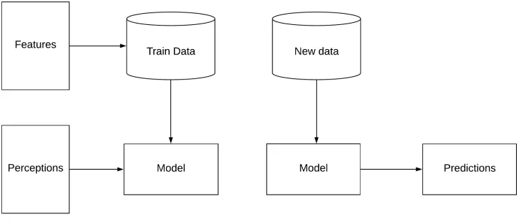
[image:13.612.121.496.247.408.2]

Based on these features a prediction model is built and data needs to be enriched to support these features. Figure 4 shows the way the previous research questions contribute to the model.

Figure 4: How the model is created and used to make predictions

RQ2 obtains the perceptions used to train the model. RQ1 finds out what features the performance of a business partner is based on, which is the definition of fea-ture engineering. What this model looks like is currently unknown therefore, the following research question is defined:

RQ3: What is the best model to rate business partners based on issue data of the iSense system?

This model predicts ratings for all business partners based on the features, how-ever not how-every indicator correlates with the rating of a business partner. For this the last research question is defined:

(14)

1.2 Approach 1 INTRODUCTION

1.2 Approach

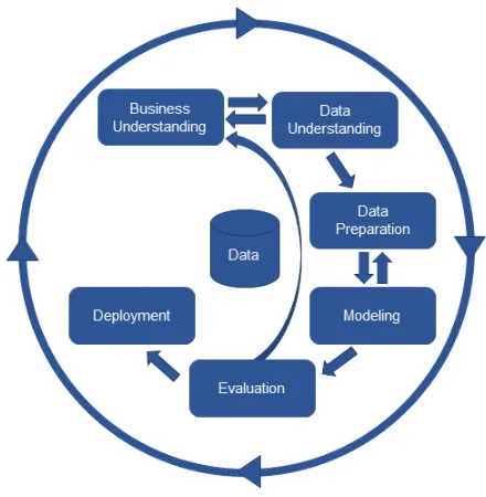
[image:14.612.193.413.273.498.2]

The purpose of this research is to create a model that predicts the performance of business partners and gives insight into the strenghts and weaknesses of the business partners. The long term goal is to allow Nedap to manage their business partners and improve their overall performance (RQ). To keep a steady structure in this thesis, we use CRISP-DM, which is a data mining model that describes the commonly process, used by data mining experts to tackle data mining problems [55]. Figure 5 shows the CRISP-DM process as described in literature.

Figure 5: The CRISM-DM process

(15)

1.2 Approach 1 INTRODUCTION

conducted in this thesis.

To enable a model to rate business partners, we first need to conduct a literature review on what the current situation is within Nedap. To achieve this we analyse what a business partner is and does for Nedap, this can be related to the busi-ness understanding part of the CRISP-DM cycle. This is followed by analysing what techniques in data analysis are commonly used for problems in this area of research.

Next, we analyse what features have an impact on the performance of a business partner (RQ1). These features come forward from literature, data exploration and interviews, this step is considered the data understanding part of CRISP-DM. Van der Spoel concluded in his research that besides looking at literature, looking at the organization and talking with experts impacts the features and new features are found [58]. To achieve this, experts are being asked about what potential features could be. Besides asking experts, the data is also being explored to find potential features of the performance, these can be validated by asking experts about their opinion on the features. The result of this is a list with features that are used by the model. However to allow the model to use these features data needs to be prepared and enriched, which is the data preparation step of the CRISP-DM cycle.

To achieve the mapping of the perception to data, the ”golden reference” needs to be known. To achieve this, we need to obtain information about the current per-formance of business partners within Nedap (RQ2). The data needs to be mapped to this perception of the truth if possible, to see if the current perception is close to the truth.

Subsequently, the model is created based on the list of features (RQ3). This pro-cess is considered the modeling step of the CRISP-DM cycle. This model will evaluate the importance of features and their relevance to the rating of a business partner. The model learns which features are important and how they relate to the performance of a business partner. To achieve this different models are tested and the best model is chosen. The definition of the best model is based on how accurate the model is in predicting the ratings.

(16)

1.3 Contributions 1 INTRODUCTION

The way this is done, is by training the model on training data. Once the model is trained, it predicts the ratings of business partners over a new period of data, which the model did not see yet. These predictions are discussed with experts to see how well the model predicts and what insights this model gives. We consider this step as evaluation in the CRISP-DM cycle. The last step is deployment, which follows if the model is correct, however falls outside the scope of this thesis.

1.3 Contributions

This thesis contributes by giving Nedap insight in the performance of business partners installing the iSense system. These insights should give understanding in which business partners are performing up to standards and which business part-ners need assistance in the transition that is currently in progress. Additionally, these insights could provide new projects to further increase data understanding and readability throughout the company.

For research in the field of data understanding and determining partner perfor-mance there were also some contributions. The methodology described in this thesis can be used to gain insight in data in most fields of research. The approach to use opinions of interviewees to train a model showed efficient in showing rel-evant parties what important features are and how important these features are. For research in performance of partners this thesis is a good example on what to expect in a similar situation and what problems can arise.

1.4 Structure

First, chapter 2 reviews different techniques in big data and data mining, which are considered for the model that is going to be build. These techniques are all commonly used in machine learning and their advantages and disadvantages are listed in this chapter.

(17)

1.4 Structure 1 INTRODUCTION

Following this, chapter 4 describes the features received from: interviews, the questionnaire, literature and data exploration. These features are used in chapter 5 as features for the machine learning model. chapter 5 also explains the choice of machine learning model and how this choice has been made. Chapter 6 discussed the validation of the model. For this the predictions the model is making are compared to the perceptions given in the interviews during the validation. Chapter 7.4 discusses the results of the model, what insights this model provided and what these insights mean for Nedap.

(18)

2 BACKGROUND

2 Background

This chapter reviews the concept of big data. It starts off by explaining what big data is, followed by the benefits and challenges in big data. The second part of the literature review describes the different techniques of data mining and ma-chine learning. This is continued by a brief description of feature engineering and concludes with a short summary.

2.1 Big Data

Over the last few years, volumes of data have increased significantly. The amount of data in 2012 is expected to have grown by 700 percent in 2018 [63]. Big data is a term for data sets that are so large and/or complex that traditional data processing software cannot properly deal with this. Where in the past big data was considered a problem, today it is seen as a huge opportunity to gain more insights into application and business information. Which leads to a new view on storing data, analyze which fields are meaningful and store as much data about these as possible. According to Zakir et al 60 percent of the respondents said that they should focus on data and analysis of this data [63]. The main goals for this would be to generate insights on customers, segmentation and targeting to improve the overall performance of the company [63]. The large amount of data stored by companies also allows for predictive analysis. Predictive analysis is the use of historical data to forecast on customer behavior and trends. The methods used to achieve predictive analysis could be by using statistical models or machine learning algorithms in order to identify patterns and to learn from this data [63]. John Walker claims in his book that many businesses use forecasting and predictive analysis in order to gain a competitive advantage [29]. He believes that the structure of an entire industry will be reshaped based on the change big data analysis will provide.

(19)

2.1 Big Data 2 BACKGROUND

to be the next ’blue ocean’ in business opportunities, meaning it can redefine busi-nesses as they are currently known [31]. Their definition of big data analytics is: ”all technologies and techniques that a company can employ to analyze large scale, complex data for various applications to augment firm performance”. These claims have recently been reviewed for the current market and situation by Gan-domi et al and concluded that the opportunities described in the past have not been fully exploited, however many are trying to do so [20].

As mentioned, the commonly used definition of big data is the three V’s. The first V is volume, volume can be defined by a variety of aspects such as counting records, transactions, tables, or files. In order for data to be considered big data the volume has to be massive, which is the case when standard processing processing software cannot deal with it anymore [59]. Laney claims that as data grows the value of an individual record decreases [32], however once the data becomes large enough the value increases since big data analytics will become possible [42]. SAP has surveyed small and middle sized companies and the results showed that 76% of the companies see big data as an opportunity [48].

One of the differences between data analysis and big data analysis is that big data analysis requires technologies that support high-velocity data capture, storage and analysis of this data. Which is the second V, velocity. Where data analysis can also be done on small data sets with simple technologies to achieve the wanted results, big data requires technologies that can handle high-velocity data capturing, stor-age and analysis of this data, such as; noSQL, machine learning and map-reduce [47] [20][59]. Big data offers a lot of possibilities when it comes to analysis. Since there is so much data it is significantly easier to detect trends and occurrences that might seem random at first, but appear to be a trend [38].

And the last V is variety. When data is received from only a single instance the amount of data can still be large, however it would still be considered data instead of big data, since the variety is small. The challenge of big data is that the data is received from many different sources and the types are different making it impossible to store them in the same database normally. This means that big data is frequently unstructured which makes it harder to do analysis on [47] [38]. Data is considered big data, when one or more V’s are present, which leads to the claim of Ward that standard processing application cannot deal with it anymore [59].

(20)

V’s is veracity. IBM claims that besides the accepted three V’s they believe verac-ity should be added [64]. Veracverac-ity is perceived by the unreliabilverac-ity to include some sources of data. For example customers often speak their minds on social media and therefore this contains a lot of valuable information. But the data is very un-certain and hard to mine. SAS sees variability and complexity as another V [49]. SAS mentions in an example that when asking two persons to measure a plant, one returns with one meter while the other says 100 centimeters. Both answers are similar yet they are described differently. This definitely could be a challenge when receiving data from many sources. Oracle supports SAS that variety should be seen as a V and adds another V, value [42]. Value should be considered as an important aspect of big data according to Oracle, since the data is of low value density, however when analyzed in large volumes it becomes worth a lot.

2.1.2 Benefits of big data analysis

Since big data has been gaining ground in the business sector it is important to know the reason businesses apply big data analysis. According to Russom any business that has involvement with customers could benefit from big data analytics on the following points [47]:

Business will have better-targeted social-influence marketing. Social-influence marketing is a new approach when it comes to marketing and this focuses on individuals rather than an entire group. These individuals are approached and get compensated for promoting the respective business. The marketing will indirectly reach an entire group that follow the individual. [47]

Not only marketing will become easier according to Russom, but customer-base segmentation will be more complete since based on this large stack of data, cus-tomers are more easily grouped in segments and categories.

(21)

digging deeper into the data the opposite can be claimed true. Since big data has advanced a lot over the years it is nowadays far easier to store this data structured in a way that allows analysis to be far more effective than before [39], not only that but Michael Ketina also supports Russoms claim that the main reason businesses are doing analysis is to gain insights into customers, market-direction and to gain new insights. These new insight can range from forecasting to analyzing the root cause of costs to fraud detection [47].

2.1.3 Barriers in big data

While the opportunities are immense, there are also some barriers and challenges in big data analytics. Russoms says that inadequate staffing and skills are the lead-ing barriers to big data analytics [47]. McAfee supports this claim by saylead-ing that there are too few data scientists in general [38]. After all, many organizations are still new to big data analytics and often correlation is being mistaken for causation which has the effect that misleading patterns are found in data and perceived as true.

Besides inadequate staff, businesses often do not support big data analysis as a program due the large concerns behind the analytics. These range from privacy concerns to cultural challenges. Michael Ketina supports these claims in his paper while adding to this that businesses need to make choices in what data to store, because otherwise the amount of data stored will grow out of control [39]. He also mentions the issue of privacy being a large risk, since the more data stored with CCTV, on the work floor and in general about the customers could give large insights in every activity that a person is doing. Privacy is something that needs to be taken in account, as business partners might not be happy that Nedap uses the data to analyze their performance.

(22)

2.2 Data Mining 2 BACKGROUND

The final point Michael Ketina is making, that is important in regards to this thesis is what is done with the results. Analysis is favored by many businesses, but it could happen that the results found can be an issue to the affected parties [39]. As explained with privacy, a business partner can fear their position if their per-formance is under standards. If this happens to be the case, caution is important and what is done with the results might need to change from what was initially planned.

2.2 Data Mining

Data mining is the analysis of (often large) observational data sets to find un-suspected relationships and to summarize the data in novel ways that are both understandable and useful to the data owner.

Hand defines data mining as the analysis of large observational data sets to find re-lationships and to summarize data in understandable and useful ways [23]. Larose supports this definition and names a few technologies that could be used [33]. Linoff even calls it a business process to find meaningful patterns and rules in large data sets [35]. There are two common goals for businesses to do data min-ing [16]:

1. Descriptive analysis, to understand what the data means and what informa-tion is stored in data.

2. Predictive analysis, to predict trends and gain competitive advantage over competitors.

(23)

2.2.1 Machine Learning

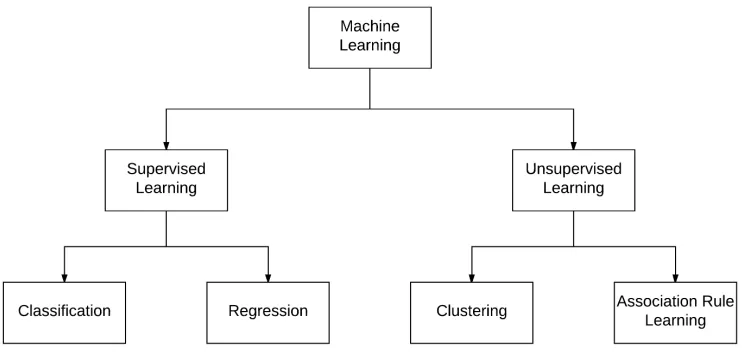
[image:23.612.121.492.283.460.2]

Machine learning is the technique of finding patterns, making predictions and ob-taining descriptive information on a data set without specifying how the computer needs to do this. There are many different models each with it’s different strengths and weaknesses [7]. Most programming languages support a machine learning li-brary and each implementation should give the same results. Machine learning is split up in two categories based on the principle the underlying algorithm is using. This division can be seen in figure 6.

Figure 6: The division of machine learning techniques and the algorithms

(24)

2.2.2 Classification

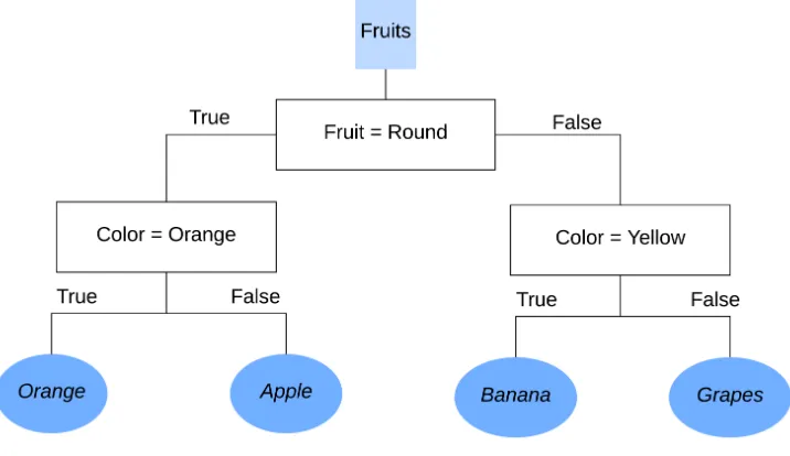
[image:24.612.127.485.385.592.2]

Classification is a technique that given labeled data constructs classes to assign samples in these predetermined groups [56]. The labeled data consists of many records and each record is unique. In order to classify data in groups a classifi-cation model is used, these can have many different forms such as a set of rules, neural networks, decision trees and many more. A classification model trains it-self on training data and constructs a model based on what it has learned. Once it has been trained it can be used to predict new samples by putting the new samples into the model, which allocates them to the defined classes.

Figure 7 shows a simple classification example. In this example there is a large pile of fruits that needs to be classified. This large stack needs to be split into four predefined categories: apples, oranges, bananas and grapes. The model identifies each fruit based on whether they are round or not. When that split has been made it can split once more on color, which splits the different fruits up in their respective classes.

(25)

2.2.3 Regression

Regression is a supervised learning method [7]. There are many different al-gorithms that work with regression models, the biggest difference compared to classification models is that regression models do not have a categorical output. This means that the prediction made by regression-models is continuous and does not limit itself to pre-defined classes (discrete) [7]. When the decision is made on supervised learning the only question that remains is to determine whether the wanted output is continuous or categorical.

2.2.4 Clustering

[image:25.612.113.501.491.630.2]

Clustering is often confused with classification. The key difference between clus-tering and classification is that clusclus-tering is an unsupervised method. Gan et al describe in their book that Data Clustering is a method of creating groups of ob-jects (called clusters) in a way that all obob-jects in a cluster are very similar to each other [19]. They are still different but share enough similarities to be considered in the same cluster. One of the key differences between clustering and classification is that the user defines what the clustering is going to be by choosing a similarity function [56]. There are common similarity functions such as k-means, k-median and min-sum [6], however the user can define its own similarity function since this is different for each domain and based on what the user assumes from the data [61].

(26)

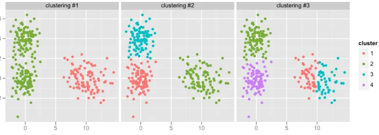
To simplify clustering again, the same example will be used as before about a stack of foods arriving. The food is not classified like before, but instead the model is used to determine samples that share features. Based on the similarity function the user defines which clusters show the best relation in the data. This could be based on clustering whether it is a vegetable or fruit or based on the colour of the food. Based on the amount of clusters and similarity function the model clusters the data. Figure 8 shows the difference the user can make by defining the amount of clusters. Each individual clustering has a different amount of clusters. The user can now look at the graphs and determine which amount of clusters best represents the samples, this example uses the same similarity function, however the user could also have tried different similarity functions.

2.2.5 Association Rule Learning

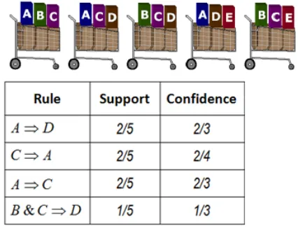
In 1993 association rule mining was introduced by Agrawal et al [2]. Association mining is the technique where relationships in the data set are built, so called associations [19]. An association is a rule which assumes there is a likelihood of a specific pattern reoccurring in the data. These patterns are defined in the form of implications such asX ⇒Y where X and Y are items within the data set. The rule should be read as when X occurs in the data set there is a high likelihood of Y appearing in the data set [25]. This likelihood of the rule applying to a case is called confidence. Besides confidence there is another statistic that is important for association mining, which is support. Support is the amount of times X appears in the entire data set. This statistic is a measurement of how often the rule might apply and how strong the rule is. The more often it occurs the more valuable the association rule is.

(27)

[image:27.612.196.409.133.298.2]

2.3 Feature Engineering 2 BACKGROUND

Figure 9: A simple association example

2.3 Feature Engineering

(28)

2.4 Summary 2 BACKGROUND

selection. There are many different techniques to do feature selection and there is no defined correct method as each case is unique as mentioned by Dash et al [12].

2.4 Summary

(29)

3 CONTEXT

3 Context

3.1 Nedap Retail

Nedap retail is a company, that has its headquarters located in Groenlo in the Netherlands and is a business unit of Nedap [41]. Nedap Retail works around the globe to deliver industry-leading products, services and solutions for their customers’ diverse needs in loss prevention, stock management and store mon-itoring. Their inventive thinking and collaborative spirit allows them to deliver tailor-made solutions for the fast paced retail sector. Below is their philosophy and text as mentioned in their manual:

”We simplify retail management while improving your customers’ shopping ex-perience. By taking most recurring tasks off your hands, we create time for you to devote to your customers. And that is what retail is all about. Whether you run a small local store or a large international chain, you will benefit from our broad range of products, ideas and services.

Nedap solutions are built upon 40 years of global experience, market expertise and close cooperation with leading retailers. Our worldwide operations are supported by a flexible network of certified partners across the globe. Nedap systems are future-proof (RFID-ready), cost-efficient and Eco-friendly. Our mission is simply to make sure your customers maintain the best shopping experience whilst we help you protect your profits. Our philosophy: ”Merchandise simply available.”” [45]

(30)

3.2 Business Partners 3 CONTEXT

an error-log. Based on this error-log the application analyze the issue that the system is reporting. The second type is called iSense [46]. The difference between iSense and OST is that iSense is an intelligent system that will analyse itself and come back with a conclusion on what is wrong with the system. Based on this information the client can easily find the problem and solve this to have their system function at maximum capacity. Since iSense is the new system from Nedap and because the old system is being phased-out this research only looks at the iSense system.

Nedap does not install the system them self and is not directly responsible for everyday problems. This is what Nedap has business partners for, what a busi-ness partner is and does is described in section ??. Nedap stores the data and has dashboards available for their business partners and their retailers to provide information about the issues arise. The information stored contains time-stamps, issue-types and duration of the issues. This is why Nedap wants to have insight in the performance of her business partners.

3.2 Business Partners

This section has been removed for public view.

3.3 Summary

(31)

4 CANDIDATE FEATURES

4 Candidate Features

This chapter describes the different techniques used to find the features for the model. The techniques used to determine the different features are: data explo-ration, interviews and the questionnaire. Each section overviews a technique used, the goal of the technique and the results of the technique. The chapter concludes with an overview of all features that are included in the model. The features obtained in different techniques are validated through expert opinions and discus-sions with colleagues.

4.1 Data Exploration

This section will take a closer look at the data set, which provides the main sources of information in this thesis. We describe what information is stored in the database, what the different fields mean, which are relevant for this thesis and conclude the section with a summary of the features that came forward. Section 2.1 discussed big data. The data used in this thesis is considered big data due to the variety and volume of the data. The data comes from several streams and databases and the volume is large as every five minutes each of the systems is sending its metrics to the servers. The challenges and barriers mentioned in the literature review are taken into account in the following stages of this research.

4.1.1 Issue categories

The issue data stored from the iSense system has a label field. This label specifies what type of issue the system is reporting. These labels can be categorized in different categories that the system is having problems with.

1. Configuration, an issue occurred that is related to the configuration of the system. Can be solved remotely.

(32)

4.1 Data Exploration 4 CANDIDATE FEATURES

3. Health, an issue that occurs when the system has problems performing. This issue might require physical support, but can sometimes be solved remotely.

4. Integration, an issue that requires Nedap to solve. This has often to do with connection to the database or the systems supporting iSense.

5. Network, an issue of this type means something is wrong with the network at the retail shop. This requires physical support to solve.

(33)

Issue Type1 Average Trimmed Average Mean Category Count type a 15014 227 10 configuration 73 type b 12857 304 648 configuration 53743

type c 7766 25 14 configuration 597

type d 2795 725 785 configuration 789

type e 792 11 5 configuration 35176

type f 4046 915 611 configuration 1258 type g 10155 29 14 configuration 1197 type h 394 124 101 configuration 21317

type i 3825 1548 1449 hardware 26228

type j 1615 8 5 hardware 4449

type k 608 9 4 hardware 25321

type l 345 30 30 hardware 17246

type m 96 31 25 hardware 41370

type n 764 14 10 hardware 469

type o 3942 213 18 hardware 26450

type p 130 12 10 hardware 13627

type q 90 10 10 hardware 250

type r 127 10 10 hardware 16247

type s 233 10 10 hardware 4595

type t 2007 10 10 hardware 1639

type u 309 10 10 hardware 49837

type v 561 388 445 health 1917

type w 246 75 12 health 1233779

type x 309 33 19 integration 50453

type y 239 60 34 integration 163039

type z 147 201 20 network 3968230

Table 1: Issue type with the statistics and category of each type

(34)

4.1.2 Responsibility

(35)

Issue Business Retail Physical Severity Type Partner Store Support Category

type a Always No No Medium

type b Always No No Low

type c Combined with Nedap No No Medium

type d No Always Always Low

type e Always No No Medium

type f Always No No Medium

type g Combined with Nedap No No High type h Always Sometimes Sometimes Medium

type i Always No Always Low

type j Always No No Medium

type k Always No No Medium

type l Always No No Medium

type m Always No No Medium

type n Always No No Medium

type o Always Sometimes Sometimes High

type p Always No No Medium

type q Always No Always Medium

type r Always No No Medium

type s Always No No Medium

type t Always No No Medium

type u Always No No Medium

type v Combined with Nedap No No Medium

type w No Always No Low

type x Always Always No Low

type y Always Always No Low

[image:35.612.125.485.126.535.2]

type z Always Always No High

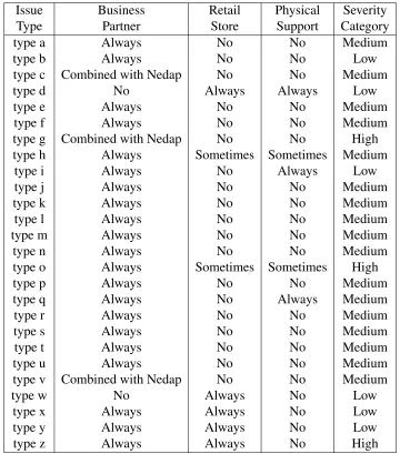
Table 2: Responsibility Matrix, responsibility against issue type with how much impact an issue type has

4.1.3 Severity Category

(36)

three categories, ranging from barely impacting the system to total system failure. Speaking with multiple experts on these issue types a list came forward with each issue type and its respective severity category. The categories with the amount of types from table 2 and the total amount of issues reported can be found in table 1. One issue type is not represented in the severity categories, which is type B. The reason for not being included in the model is that this issue type can be triggered by multiple parties to temporarily mute the system to fix existing issues. According to experts, these issues are impossible to track whether it was done to prevent issues from occurring or to solve problems. The impact of this issue type is little as it is most often used to deploy a firmware update or configure the system at installation.

4.1.4 Issue duration

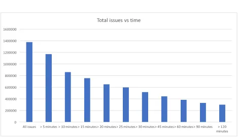
The table that stores the issues has two fields: ”reported at” and ”resolved at”. By using these two fields the duration of issue can be calculated. The combination of the severity category and the issue duration show the impact the reported issue had on the system. Without issue duration it is impossible to relate the issue data to the performance of a business partner, as their main responsibility is ensuring the system performs optimally. The exploration showed there were a large portion of issues that were resolved within ten minutes, which can be seen in figure 10. Important to notice is that there are a lot of issues that are under ten minutes.

Initially the idea was to exclude issues below ten minutes, since these would not require any manual effort. However, in the pre-research an issue came forward with the framework analyzing the issues. Because of this, issues could be resolved when the issue still existing and then re-opened. This means that issues below ten minutes could actually be a long list of issues happening consecutively. Therefore the conclusion is that all issues are summarized as the total issue duration.

4.1.5 Issue count

(37)

[image:37.612.71.540.104.373.2]

Figure 10: Total amount of issues above the duration on the X-label

duration is included as an indicator on how a business partner is performing.

4.1.6 Stores, devices and gates

We discussed issues in the previous sections and how these fall in different cate-gories. Each of these issues can be related to three severity levels as mentioned in table 2. Figure??shows that a business partner manages stores. These stores can have one or multiple devices running the infrastructure. In this diagram the de-vices are iSense dede-vices. iSense can have a small system consisting of two gates, or a complex system containing as many as the retailer wishes for.

(38)

between business partners, issue durations and counts need to take this in account. It is clear that a business partner with more stores, will have more issues and a longer total duration. Therefore the amount and duration of an issue is related to the amount of gates. This assumes that more gates will cause more issues, which sounds logical and according to colleagues is likely true. Therefore, the amount of gates is considered a feature.

Discussion with account managers and sales representatives brought up the rel-evance of the amount of stores. Business partners with many stores need more personnel to solve issues that require physical presence. They also need more personnel in general to handle issues that come up and pose a higher risk of hav-ing unemployed personnel, since recruitment continues to grow for these business partners. A possible scenario is that a business partner will have long unresolved issues, which could be related to lack of personnel to handle this. Therefore we include the amount of stores as a feature. There is no data available on the amount of personnel a business partner has, this could eventually be obtained and in future added to the model to show this. For now we include the amount of stores as an indication on how large a business partner is.

4.1.7 Summary

This section discussed the data exploration. Based on the data exploration a few features came forward which are the following:

• Severity category - categorical (high/medium/low)

• Issue duration - integer of total minutes

• Issue count - integer

• Amount of stores - integer

• Amount of devices - integer

(39)

4.2 Interviews 4 CANDIDATE FEATURES

4.2 Interviews

This section describes the goal of conducting interviews for this thesis, the ap-proach used in the interviews, who has been interviewed, the result of the inter-views and a discussion. The section concludes with a list of indicators that have been added to the results from previous section.

4.2.1 Goal

During the data exploration many candidate features came forward, which could not be confirmed to have an impact on the performance of a business partner due to lack of knowledge on the subject. One of the goals of the interview is to analyze the assumptions with the interviewees. If an assumption has influence on the performance of a business partner, said assumption is included in the list of indicators. The second goal of the interview is to have a large diversity of opinions to have a complete view on the performance of a business partner. The third goal of the interview is to create discussion within Nedap on what indicators have impact on the performance of a business partner. The way this is done is by validating opinions of previous interviews in the next interview. The main reason to validate opinions is to ensure the indicators are general indicators and not specific for a function or person.

4.2.2 Approach

(40)

parts, which are defined as following:

• Introduction

• Discussion and validation

• Actual performance

Each interview starts with a brief introduction into our research, following into an open question asking what they believe indicates the performance of a business partner. During the interview questions are asked to let interviewees elaborate or to create a discussion with opinions from previous interviews. The interview ends with the same set of questions each time, which is to rate 15 business partners on a scale from 1 to 10. These ratings can be elaborated during the interviews, to get an indication on why some business partners are getting higher or lower ratings than others. These ratings are used by the model as input data and are expanded by conducting a questionnaire, which is discussed in the next section. The way these 15 business partners have been chosen is elaborated in the section of the questionnaire.

4.2.3 Interviewees

As mentioned in previous sections the diversity of the experts that are interviewed is important to ensure all parts of performances have been discussed. To achieve this we conduct interviews with many different teams and from different conti-nents. Different continents is important to ensure that the opinion of Nedap US and Nedap China is similar and that there are no indicators that are only relevant to a specific region. The interviewees are from the following teams:

• Account managers

• Developer services team

• Sales director Asia

• Pre-sales

• Business partner manager

(41)

Since technical operations has regular contact with the business partner on issues, assist business partners if necessary and work with the data used in this thesis, we interview two members of the technical operations team separately to see if they both agree with each other. All interviewees are currently working within Nedap except for the business partner manager, who recently moved to another company. The teams that are not represented in the interviews are R&D and hardware on iSense. The reason for not including them in the interviews is that when briefly speaking with them, they mentioned they have no insight in performance of a business partner and only focus on the performance of iSense as a system.

4.2.4 Results

The transcripts of the interviews can be found in appendix A. The diversity of the interviewees resulted in many different aspects that might be relevant as features for the model. In order for a feature to be included in the list of features, a feature had to meet the following criteria:

1. Related to iSense

2. Can be found in data

3. Validated by other interviewees

If a feature cannot be found in data, it could still be a great addition to the system in the future, these features are discussed in the future work section. Similarly, features not related to iSense can be additions when a similar model is being cre-ated for the other systems within Nedap. These features are also discussed in the section future work. Below is a description of each feature, why it is relevant for this thesis and what the arguments of the interviewees are to include the mentioned feature.

4.2.4.1 Communication

(42)

systems and that they are working on this. Secondly, the business partner needs to have an open communication with Nedap about problems with the systems when they cannot solve the issues, have problems recurring and have feedback about the system. The communication between the business partner and the retailer is external and no data is available to include this as a feature. The communi-cation towards Nedap does exist in a database, which is called Freshdesk [18]. Freshdesk store all tickets that are submitted by business partners, with priori-ties, type of question and many other fields. These tickets indicate how much a business partner is communicating with Nedap. The interviewees mentioned that communication is neither bad or good, some business partners communicate a lot to give feedback, which is good. However, there are also business partners that communicate a lot, but ask simple question which should be known information. The way this is currently stored in Freshdesk, it cannot be related to performance yet, however improvements to this are being worked on. Ideally, the feature would be included as a categorical field, which indicates how well the communication of a business partner is. Since this requires significant changes to the existing system and transformation of the existing data, it is excluded from this thesis.

4.2.4.2 Training

(43)

other employees can follow e-learning to further train their knowledge. Based on this, the features e-learnings and physical training are included.

4.2.4.3 Global vs Local

As discussed in chapter 3, a business partner has two different type of retailers that they serve. On the one hand are the globals, which are given to the business partner by Nedap. On the other hand are retailers that they find themselves. Interviewees were asked to answer a question on whether global retailers are just as important as a local store for Nedap. Many interviewees said that every store should be equal. However, when asked if two retailers have an issue at the same time who should be helped first, many interviewees said that obviously the global should have priority. We had the assumption this was the case and during the interviews it became clear that global retailers are treated differently. Based on the input that came forward in the interviews, retailers are separated in two groups. The first group are all global retailers of Nedap, the second group are the ”local heroes” that the business partner found them self. These groups each have the same amount of indicators, but are separated under the assumption that business partners treat the globals different.

4.2.4.4 Performance time window

Every interview ended with the set of questions, to score a business partner on a scale from one to ten. In order to make these ratings meaningful, we asked each interviewee whether the performance of a business partner was stable over a period of a year. Each interviewee said that the performance should be close to steady over a year. They mentioned a business partner can slightly improve or get worse, but generally they can see a steady performance. To see which model best represents the perception that lives within Nedap, different time windows are tested. And the time window that best represents the perception is going to be used. Eventually, Nedap wants to see the performance of a business partner over the last three months to determine whether actions they took had influence on the performance of a business partner. The time windows that are tested by the models are:

(44)

4.3 Questionnaire 4 CANDIDATE FEATURES

• Three month interval

• Monthly interval

4.2.5 Summary

This section started by explaining the goal of the interviews, the approach, who the interviewees are and concluded by explaining which features were added to the list and their arguments. The feature list has been extended with the following features:

• Physical training X years ago - integer

• E-learning - integer - amount of e-learnings completed

• Split between global and local - all existing features are split up in two groups

• Different time windows

Next section describes the questionnaire that has been conducted and it elaborates how the last part of the interview came to its definition as it is the questionnaire, but with the opportunity to elaborate the ratings.

4.3 Questionnaire

This section describes the questionnaire that has been conducted. The section starts with an explanation on the goal of the questionnaire, followed by explaining the questions of the questionnaire and concludes with the result of the question-naire.

(45)

trains on these ratings and attempts to predict the ratings of business partners that have not been rated on new, more recent, data.

The questionnaire asks experts to score a set of 15 business partners on a scale of 1 to 10. These 15 business partners are selected on the following criteria:

• More than 50% of their systems using iSense

• More than 20 devices

• Multiple regions

The first criterion is important, since it allows us to relate the ratings to iSense rather than it most likely being related to the old OST system. The second criterion ensures that a rating can be given on a business partner. 20 devices indicates that a business partner has had a few stores for a while now. The last criterion is to ensure that the inputs received verify the assumption that came forward during the interviews, which is that region is irrelevant. During the interviews it became clear that while region often matters, in this case the performance of a business partner should not depend on the region. To verify this, the business partners asked in the questionnaire are from different regions. The model should also predict the ratings of these business partners correctly based on the training data.

Statistic Result

Number of business partners with more than 50% iSense 20 Number of business partners with more than 20 devices 15

and 50% of their systems iSense

[image:45.612.139.474.463.568.2]

Total Number of iSense devices within this group 1260 Total Number of devices in this group 1794 Percentage of iSense devices compared to the total 33.77%

Table 3: Issue type with the statistics and category of each type

(46)

training data, because the group of participants is broad enough to obtain enough ratings for each partner. In combination with the interviews, the goal is to get input from 20 different parties. Under the assumption that each participant on average rates half of the business partners, we would have 150 input ratings for the model to train on.

4.3.2 Data

The questionnaire asked interviewees to rate business partners over the last year. The performance of a business partner is steady according to interviewees over a year, with a few peaks and dips. The questionnaire should be conducted every three months to obtain more data for the models to train on. This means for the val-idation of this research only one questionnaire is conducted. As mentioned there were 148 responses, which is the input set for this thesis. In future every three months a questionnaire or other method should be conducted to keep increasing the input-set for a model to train on.

All features use data from the specified period. The model determines which time-period is the best, which is done in a later section. The features found in this section that are related to issues (count and duration) are only from the period given to the model. The amount of stores, devices, gates are based on data from the start of the system, however within the period this amount could show an increment. Physical training is updated on the day a physical training has been completed, therefore can fall within a new period. E-learnings is the total amount of e-learnings completed that are currently active. Some e-learnings are outdated and are updated in the system as outdated. The feature excludes e-learnings that are no longer relevant for the time-period.

4.3.3 Results

(47)

Business2 _Minimum _Maximum _Average _Res- _Standard

Partner Rating Rating Rating ponses Deviation

Business partner 1 3 7 5,86 7 1,491

[image:47.612.112.500.125.383.2]

Business partner 4 5 9 7,50 14 1,082 Business partner 5 5 8,5 6,70 10 1,003 Business partner 6 4 8 6,42 12 1,068 Business partner 7 5 8 6,62 13 0,842 Business partner 8 4 8 5,96 12 1,130 Business partner 9 5 8 6,50 12 0,891 Business partner 10 5 9 7,33 6 1,724 Business partner 11 5 9 7,67 6 1,247 Business partner 12 2 7 5,29 12 1,388 Business partner 13 5 6 5,25 4 0,433 Business partner 14 2 7 5,08 12 1,622 Business partner 15 5 8 7,14 11 0,867

Table 4: Business partners ratings from questionnaire and interviews

While some business partners are rated fairly similar with a potential outlier, there are some business partners which opinions are fairly different, for example busi-ness partner 9, where the average is precisely in the middle of both the minimum and maximum. This is one of the main challenges of the model, since it needs to determine which of the rating is correct, if at all correct.

4.3.4 Summary

This section described the questionnaire that has been conducted. We discussed what the goal of the questionnaire was, what the questions in the questionnaire were and the results that came forward. Next section concludes the features found in this chapter.

(48)

4.4 Data preparation 4 CANDIDATE FEATURES

4.4 Data preparation

In order to include some of the features that come forward in this section, data needed to be prepared. The amount of gates is a data row that was recently added to the system. Due to the firmware some systems did not report the amount of gates to Nedap and this means there are a few devices that have no amount of gates reported. Discussion with experts about the amount of gates resulted in taking two gates as a default value. The minimal amount of gates a system needs to have is two, the assumption made here is that the retail stores that do not have the right firmware are likely the smaller retail stores. The average amount of gates in the field was 2.65 and the experts that the larger systems have reported their gates. Which is why two gates would best represent the situation.

Currently, global customers are not stored in a database. However, sales know the names of the retailers that are global retailers. To make sure the data can be split in the two categories an additional column has been added to the local data set that matches the string names of the global retailers.

The amount of stores and devices also needed to be limited. In the data set are also devices that are no longer active or stores that have been blocked. These needed to be filtered out to only show the relevant devices and stores. Secondly, the data set also contained OST systems. Both these situation have been filtered out in the data set by using the existing infrastructure and fields to filter them.

4.5 Conclusion

(49)

4.5 Conclusion 4 CANDIDATE FEATURES

Feature Type Value Definition

Amount of stores Integer Total amount of iSense stores Amount of devices Integer Total amount of iSense devices

Amount of gates Integer Total amount of iSense gates Physical Training Integer Years since last training

E-learning Integer E-learnings completed Issue duration high severity Integer Total minutes a system is down

Issue count high severity Integer Total amount of issues Issue duration medium severity Integer Total minutes a system is down

Issue count medium severity Integer Total amount of issues Issue duration low severity Integer Total minutes a system is down

[image:49.612.117.485.127.304.2]

Issue count low severity Integer Total amount of issues

Table 5: An overview of all candidate features, these are repeated for local retail-ers and global retailretail-ers

(50)

5 THE MODEL

5 The Model

This section describes the choices made in creating the model. First, we discuss the approach that is used to create the model, the reason for using this approach and what the pitfalls of this approach are. Following this, we discuss the different models within this method, the advantages and disadvantages of each model and conclude by elaborating the chosen model.

5.1 Approach

The goal of this thesis is to predict the performance of business partners based on a set of indicators. Chapter 2 discussed machine learning, which is the model that is going to be used. The reason for using machine learning is that the goal to predict the performance of a business partner is best executed by machine learning as discussed in chapter 2. There are many languages that support machine learning, however for this thesis we use Scikit, as the models have been validated in other researches and Python is a known language to us [43]. Previous section discussed the questionnaire that was conducted to obtain ratings of a set of business partners, these ratings are needed to predict new ratings for all business partners. Since predicting is one of the goals of this thesis, supervised machine learning is used. Supervised machine learning requires labeled data to work and the input of the questionnaire can directly be used as labels for the model.

Chapter 4 described the indicators that came forward during data exploration and interviews. These potential features are used in the machine learning model. Chapter 2 discussed feature engineering and the steps that fall under feature engi-neering. Machine learning determines, which of the features give insights in the performance of a business partner.

(51)

5.1 Approach 5 THE MODEL

insight in how it got to its predictions. For Nedap a prediction is irrelevant when it cannot be explained, but the accuracy of the rating still has to be high. To not limit the model to only white-box models, a dashboard is created which shows the rating of the business partner in question and all features with their values, rela-tive position (ranking compared to other business partners) and the time-window. This is to ensure that if the model were to make an incorrect prediction, it would show the used data and the rating can be ignored. This dashboard also shows the respective weights of each feature as determined by the machine learning model. This allows us to freely choose between white-box models and black-box models.

The last choice made on the method of machine learning is the choice between a classification problem and a regression problem. During the interviews it came forward that differences between business partners can be small. Classification would mean that business partners are grouped in pre-defined classes. Since dif-ferences between business partners can be very small, we chose for regression. Regression models give a decimal precision prediction, making them more valu-able than classification. Secondly, since the ratings used as labels differ a lot, as can be seen in table 3, a prediction in decimals will give a better representation of the truth.

(52)

5.1 Approach 5 THE MODEL

results in the model not being able to capture the underlying trend [9]. Based on the literature and research conducted in this area, the definitions for overfitting and underfitting are as follows:

• Overfitting occurs when the model has too many variables or too little data to capture the underlying pattern

[image:52.612.115.499.289.386.2]

• Underfitting occurs when the model has too little variables or features are too generic to capture the underlying pattern

Figure 11: Visualization of overfitting and underfitting

It is important to have a correct fit. Overfitting and underfitting has been visual-ized in figure 11. The figure shows what a machine learning model does when it underfits and overfits. Ensuring a correct fit is a challenge that is going to be tackled by using different models and parameterizing the models well. Besides this, there are methods that help ensuring a correct fit such as feature reduction (reducing the set of features to exclude noise). These are discussed in later stages of this thesis.

5.1.1 Summary

(53)

5.2 Models 5 THE MODEL

5.2 Models

As discussed in last section, the model should be a regression model. This limits the amount of possible models. First, we determine a long-list which is a list with models applicable to this case. Following this, a short-list is determined on a set of criteria. The shortlist candidates are thoroughly tested and optimized. To find the best model, we use accuracy and consistency. The accuracy of the candidate models describe how well it can predict the test data and consistency describes the performance over multiple iterations. The consistency is good when the model is stable and not related to the received test/train data.

5.2.1 Data scaling

For regression models to work, it is important to scale data so that the model does not base its conclusions on the feature with most variance [50]. This is important, since the range of the defined features differ a lot. Some of the proposed tech-niques filter outliers. Filtering outliers is not wished for in our case, since if a business partner is under performing this business partner needs to be rated lower on that feature. The choice in this thesis has fallen on a MinMax scalar. A Min-Max scalar transforms all data to the given range. This technique compresses the data in the center and outliers are still on the outer edges. The way the MinMax-scalar scales the data can be seen in figure 12. In the figure the range is 0 to 1. In our model a range of -1 to 1 is used.

5.2.2 Multiple perceptions

(54)

[image:54.612.102.497.128.306.2]

Figure 12: An example how a MinMax-scalar scales the data

5.2.3 Long-list

As mentioned before, Scikit is used in this thesis [43]. Scikit has Sklearn available in python, which is a library that has validated implementation of many machine learning algorithms. The long-list, that this section describes is the complete list of supervised regression models in Sklearn [52] as can be seen below:

• Generalized linear model

• Linear and quadratic discriminant analysis

• Kernel ridge regression

• Support vector machines

• Stochastic gradient descent

• Gaussian Processes

• Cross decomposition

• Naive Bayes

• Decision trees

• Ensemble methods

• Multi-class and multi-label algo-rithms

• Isotonic regression

(55)

another classifier and run this multiple times. This means that if any of the models is able to fit, this model will also be able to fit. Since implementation of a model is very simple in Sklearn, every model is implemented and checked on whether it meets a set of criterion. These criteria are discussed below.

5.2.4 Criteria

The first criterion is that the model can fit itself with the amount of data that is available. Some models require a large amount of data in order to converge properly. These models cannot be included in this thesis, since the amount of data that has been rated is sparse. To detect that a model did not converge, two methods have been found. The first method is that the model will constantly predict the same value or close to the same value. The second method is that the models requires a very large amount of iterations, that the amount of data provided cannot ensure that each iteration has unique data. When a model sees the same data multiple times, it is very likely to overfit and therefore excluded.

The second criterion that is considered in choosing a model is the output of the model. Models are not restricted in their prediction. Some models fit the test data accordingly, however when the test data is not in range of the train data they predict values far out of the wanted range of ratings. These models cannot be included, because the output of a model needs to be a rating between one and ten.

(56)

5.2.5 Short-list

The biggest batch of models did not make the short-list, because they could not fit properly. These models are known to require a lot of data to fit. Since, the sparsity of data exists in this thesis these models are excluded. Some models have problems predicting values within a given range and gave results with large negative or positive values. Therefore, these models are also excluded since they did not meet the second criterion. Table 6 shows on what criterion the different models failed to pass.

Model Able to fit Predict within range Generalized linear model X

Linear and quadratic discriminant analysis X Kernel ridge regression X

Support vector machines X

Stochastic gradient descent

Gaussian Processes X

Cross decomposition X

Naive Bayes X

Decision trees X X

Ensemble methods X X

Multi-class and multi-label algorithms X

Isotonic regression X

[image:56.612.112.502.274.487.2]

Neural networks X

Table 6: Accuracy percentages by different cases

(57)

5.2.5.1 Regression tree

A regression tree is the same as a decision tree, except that it allows its predictions are a continuous output (regression) allowing it to predict values that have not been specified in the training data [51]. A regression tree works by making rulings, to which each set of features is compared. A ruling always looks like the following:

feature name <=value of feature

Based on the features each individual sample is given a value true or false. True values continue left in the tree, where false values continue to the right side. This can be see in figure 13, where the ruling that has been made is that ”medInc” is lower or equal to the value 5.04. If this is the sample, the set of features will continue left, otherwise they go the right side of the tree. Eventually a regression tree reaches the bottom where a value is assigned to the given sample. Figure 13 clearly shows that when the feature ”medInc” is high the sample is given a high score. These value assignments are called leafs and is one of the main methods to prevent overfitting in a regression tree. In Scikit there is an option to define the minimum amount of samples a regression tree needs to have in order to split into a leaf.

The way a regression tree predicts new samples is that the data of the new sample is held against the trained tree and the new samples will eventually reach a leaf, which assigns a rating to the samples. For a regression tree it is very important that data is always in the same range, otherwise the rulings will not work as the dimensions changed.

5.2.5.2 Gradient Boosting Regressor

(58)

[image:58.612.131.474.153.338.2]

[image:58.612.115.496.422.639.2]

(59)

5.3 Feature selection 5 THE MODEL

in a different output and a new error rate. This new attempt is continued until the specified amount of attempts have been reached or the loss becomes larger multiple times in a row, in which case it stops early. When the model completed his fitting, it will use the average of all trees as output. Which is why a gradient boosting regressor is known to be very robust to overfitting as it continuously maps the loss to the next tree.

Since the underlying algorithm of a gradient boosting regressor is a regression tree, its predictions work the same except that it consists of the result of many regression trees. While this model looks very similarly to the regression tree, the predictions the model makes are very different.

5.2.6 Summary

This section discussed the choice of scaling method in this thesis and why data needs to be scaled. Following this, the different models that are applicable to this thesis are discussed and two candidates came forward that met the defined criteria, regression tree and gradient boosting regressor. Next section discusses what criteria determine the final model and which of the candidates is chosen.

5.3 Feature selection

Before the choice of a model can be made, the candidate features need to be ana-lyzed and determine whether each feature is relevant for the models to determine predictions on. The data consists of the features described in section 4. Since there might be correlations between the different features and the data is sparse for the amount of features. To allow the models to fit on the sparse data, the features are reduced this is done using Principle Component Analysis (PCA). Two definitions of PCA are as follows:

• ”PCA is a multivariate technique that analyzes a data table in which ob-servations are described by several inter-correlated quantitative dependent variables” [1]

Predicting the performance of business partners, using issue data of the iSense system : mapping a perception to data using machine learning

Abstract

Preface

Contents

List of Figures

List of Tables

1

Introduction

1.1

Objectives

Problem statement

1.2

Approach

1.3

Contributions

1.4

Structure

2

Background

2.1

Big Data

2.2

Data Mining

2.3

Feature Engineering

2.4

Summary

3

Context

3.1

Nedap Retail

3.2

Business Partners

3.3

Summary

4

Candidate Features

4.1

Data Exploration

4.2

Interviews

4.3

Questionnaire

4.4

Data preparation

4.5

Conclusion

5

The Model

5.1

Approach

5.2

Models

5.3

Feature selection