Gravity model parameter calibration for large scale strategic transport models

(1)

Gravity model parameter calibration for large scale

strategic transport models.

Mark Pots

Company supervisors: Bastiaan Possel, Luuk Brederode and Nico Aardoom

University supervisor: Peter J.C. Dickinson

Graduation supervisor: Marc Uetz

Chair: Discrete Mathematics and Mathematical Programming (DMMP)

Applied Mathematics

(2)

Abstract

This study considers the calibration of the lognormal cost function parameters within the simultaneous gravity model for large scale strategic transport models. The parameters are calibrated based on observed trip length distributions and modal split fractions. First the full trip distribution used at Goudappel Coffeng that consists of a stratification in trip purposes and sub purposes is described in detail. A new calibration approach is in-vestigated that proposes a triproportional fitting procedure over the current biproportional fitting procedure. The triproportional fitting procedure solves the gravity model equations while simultaneously fitting the trip distribution on modal split. This simplifies the calibration eliminating the modal split constraint and its associ-ated lognormal parameters. Under the new approach the calibration algorithms’ running times are considerably reduced.

(3)

Notation

Globally used indices:

i a zone of origin

j a zone of destination

m a mode, e.g. m∈ {car, bike,public transit}

u a user class, e.g. u∈ {co (car owners),nco (non car owners)}

k a cost bin

Globally used Variables:

tijmu number of trips made from zoneito zonej using modemby trip

makers in user classu

Tm _{OD matrix for mode}_m

T either denotes a full trip distribution i.e. a distribution ofT over

all thetijmu’s

or the OD matrix aggregated over all modes: T =P

mT

m

Pi(u) production value of zone ii.e. the observed number of trips

de-parting from zonei (made by user classu)

Aj(u) attraction value of zoneji.e. the observed number of trips arriving in zonej

Oi(u) production balancing factor of zonei

Dj(u) attraction balancing factor of zonej

Fmu(cijm) cost function to be calibrated, models the willingness to travel

using mode m at generalized costs c by a trip maker from user

classu

cijm (generalized) cost to travel from zoneito zonej using mode m

αmu (lognormal) cost function parameter for modemand user classu

to be estimated in the calibration or balancing factor for modem

and user classu

βmu (lognormal) cost function parameter for modemand user classu

to be estimated in the calibration

b

dmuk observed number of trips made by modem by user class uof a

cost in bink

dmuk modelled number of trips made by modem by user class u of a

cost in bink

d

M Smu the observed fraction of trips made using modemby user classu

(6)

1 Introduction

This thesis is the final result of my graduation research at Goudappel Coffeng. The goal of this research was to improve the automatic parameter calibration of the gravity model that exists within the transport planning software package Omnitrans. The emphasis is on gravity models within large scale strategic traffic models. The gravity model for trip distribution is based upon Newton’s gravity model. It generates a trip distribution over the zonal grid of the strategic traffic model. The most important element that determines this distribution of trips is a cost function inside the gravity model. The calibration considers the parameters of this cost function.

This section gives an introduction to the framework and context in which this research is done. Section 1.1

describes some basic trip properties which form the dimensions of the trip distribution resulting from the gravity model. Section1.2describes the four-step traffic model, which is the larger transport modelling context within which the gravity model is an important component.

1.1 Trip numbers

The strategic traffic model we deal with considers a study area which is assumed to be partitioned into a set of n zones i.e. a zonal grid. In the trip distribution model we are concerned with the origin and destination of trips as well as the mode by which the trip is made. We usei to denote a zone of origin from which a trip starts andjto denote a zone at which a trip ends. We use the indexmto denote a mode of transport by which a trip is made. Examples of modes of transports include car, bike or public transit.

We have described three properties a trip has in the trip distribution model so far: a zone of origin, a zone of destination and the mode of transport by which it is made. Another trip property we are interested in is the person who makes the trip. We can partition the population of trip makers into groups so that in a group all the trip makers share one or more of the same properties. These groups we will call user classes and we useu

to denote a particular user class. We can for example divide trip makers in the user classes of trip makers who own a car and trip makers who do not own a car: u∈ {co, nco}.

With these indices we can specify the number of trips with certain properties. By the trip number

vari-abletijmuwe denote the number of trips that are made from zone ito zonej by a trip maker from user classu usingmas a mode of transport for each pair of zones (i, j), modemand user classu. Together all thetijmu’s form the trip distribution.

1.2 The four-step traffic model

(7)

i

j

i

j

i

j

t

ijm1

t

ijm2

t

ijm3

t

ijm

Trip generation:

Destination choice:

Mode choice:

[image:7.595.134.458.103.388.2]

Route choice:

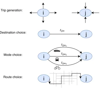
Figure 1: Steps of the four-step traffic model.

One - Trip generation:

The objective of the first step is to determine for each zone how many trips should have their origin (departures) and destination (arrivals) in that zone. The number of trips that have their origin in a particular zone is called the production of that zone while the number of trips that have their destination in that zone is called the attraction.

Two - Destination choice:

The second step matches the production and attraction values to get a trip distribution specifying the number of trips that go from each origin zone to each destination zone. Other than the production and attraction value of an origin-destination pair the main factor determining this trip distribution is travel impedance meaning roughly speaking the time and distance it takes to travel the trip.

Three - Mode choice:

The third step of mode choice, also called modal, split further refines the trip distribution resulting from the second step by determining for each trip which mode of transport is used.

Four - Route choice:

(8)

such as traffic engineers and municipalities.

Usually at Goudappel Coffeng, and so is the case in this thesis, steps two and three, destination choice and mode choice, are combined in one trip distribution model which does both steps simultaneously. For this reason the specific trip distribution model we will be considering, which is a gravity model, is called a simultaneous gravity model.

This thesis will not explain the first step of trip generation other than mentioning that both production and attraction values are generated in an exogenous model based on socio-economic data. Therefore we assume the production and attraction values from this step to be readily available data in the next step of trip distribu-tion. For a more thorough explanation on the trip generation and traffic assignment phase and a more through treatment of the four step model in general we refer to Ortur and Willumsen[5].

The goal of this research is to improve the calibration of cost function parameters of the simultaneous gravity model for large-scale (thousands of zones) strategic traffic models. Performance measures were established on which the developed methods were tested on. In particular we implemented gradient based methods and com-pared their performance with the original hillclimbing algorithm.

Structure of the remaining thesis

(9)

2 The simultaneous gravity model

The purpose of this chapter is to review the simultaneous gravity model within the four-step model. The simultaneous gravity model is the key building stone of the full trip distribution models that we review in chapter 3. Section 2.1 introduces a doubly constrained simultaneous gravity model for uniform trip makers. Section2.2discusses the choice of deterrence function that can be made inside the gravity model. The calibration of this deterrence function is the main research subject. Section2.3 presents a mathematical derivation of the gravity model. Section 2.4 describes the solution method for the gravity model which is the biproportional fitting procedure and reviews some of its properties.

2.1 Doubly constrained simultaneous gravity model

This section describes the doubly constrained simultaneous gravity model. Wilson[15] founded the gravity model approach to trip distribution modelling. To simplify matters and to cater for the reader with no background knowledge on gravity models we first introduce a simultaneous gravity model in which the population of trip

makers is assumed to be uniform. Therefore the index u for user classes is omitted for now and the model

discussed here computes the trip distributiontijm. The model computes a trip distribution based on trip-end values, generalized costs and a definition of the deterrence functions.

2.1.1 Trip-end constraints

The trip-ends consist of production and attraction values obtained from the trip generation step. Denote by

Pi the production value of zone iand denote by Ai its attraction value. As mentioned before: the production value of a zone represents the number of trips that should originate in that zone while the attraction value represents the number of trips that should have their destination in that zone. This is encapsulated by the trip-end constraints:

X

m,j

tijm =Pi for eachi (1)

X

m,i

tijm=Aj for eachj

The gravity model is called doubly constrained if both production and attraction constraints are required to be met. Singly constrained models only require one constraint type to be met. The trip-end data can also be omitted or simply unavailable in which case the model is called unconstrained. So the choice of gravity model in terms of it being singly (origin or destination based), doubly or unconstrained depends on the level of knowledge in trip-ends.

2.1.2 Balancing trip-end values

Denote by T the total number of trips modelled i.e. the sum of all the tijm. It follows from the trip-end constraints (1) that:

X

i

Pi= X

i X

m,j

tijm=T = X

j X

m,i

tijm= X

j

Aj

However, the left- and right-hand side can be unequal in case the production model and attraction model (together forming the step of trip generation) are inconsistent1_{. This inconsistency can be corrected by a simple} preprocessing step called balancing. Balancing simply means to either scale the production values such that

1_{In practice this depends on the time period that is modelled for. For a time period of a full day the productions and attractions}

(10)

their sum matches the sum of attraction values or to scale the attraction values to match the total production sum. Which sum we hold as valid is determined by comparing the reliability of the models for productions and attractions. For example in case we trust the production values more we scale the attraction values towards adjusted valuesA0_j by:

A0_j = P

iPi

P

iAi

!

·Aj

2.1.3 Generalized costs

Intuitively one would in general expect more people to travel between two locations given it is easier to make the trip. This is where the second main input to the gravity model of generalized travelling costs come in to play. Denote by cijm the generalized cost to travel from zone i to zone j using m as a mode of transport. Practically speaking the units of these costs can be anything from time, distance, energy or money hence they are called generalized costs. The generalized costs can also be a linear combination of these numbers by applying appropriate conversion coefficients. For example it is possible to express generalized costs in purely monetary units from travel time and travel distance in case we have knowledge of the value of time and fuel costs.

2.1.4 The gravity equation

The gravity equation can now be introduced by:

tijm=piajPiAjFm(cijm) (2)

Here pi ≥ 0 and aj ≥ 0 are called balancing factors which need to be determined so that the trip-end

constraints hold. The cost function Fm₍_._{) is mode specific and acts on the generalized costs to model the} willingness to travel at a certain (generalized) cost. The cost functions are also called deterrence functions.

We can rewrite the gravity equation (2) in a simpler form by a change of variables: Oi = pi ·Pi, Dj =

aj·Aj:

tijm=OiDjFm(cijm) (3)

We will actually use this equation as the gravity equation and by balancing factors we will mean these

Oi’s and Dj’s. However the form of equation (2) is useful to observe three assumptions that are built into the gravity model. Namely that the number of trips between a zone of origin iand a destination zonej made by mode mis proportional to the observed number of departuresPi from the origin zonei, the observed number of arrivalsAj to the destination zonej and also is proportional to a cost function factorFm(cijm) representing the willingness to travel at the cost to travel from zoneito zone j by mode of transportm.

i

j

i

j

i

j

tijm1

tijm2

tijm3

tijm

Trip generation:

Destination choice:

Mode choice:

[image:10.595.217.400.573.643.2]

Route choice:

(11)

2.1.5 Resemblance with Newton’s law

The gravity model of traffic is similar to Newton’s law of universal gravitation therefore lending its name from it. Newton’s gravitational law states that the gravitational pull between two objects is proportional to the mass of the first and second object and also is proportional to the inverse square of the distance between the objects, see figure 3. The gravity model of traffic usually uses a more general cost function howeverFm₍_c

ijm) =c−ijm2

[image:11.595.242.353.249.320.2]

has been used in some models as a cost function. One way in which the analogy between Newton’s law and the gravity model of traffic breaks down is that in Newton’s law the calculated force works bidirectional i.e. the force object one exerts on object twoF2 is equal to the force object two exerts on object one F1 while we do not have tijm =tjim necessarily. Since the costs to travel on the way incijm and on the way outcjim do not have to be equal and neither do the production and attraction value pairs.

Figure 3: Newton’s law of universal gravitation.

2.2 Deterrence functions

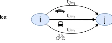
Different choices of cost functionsFm₍_c

ijm) are available. The choice of the cost function has a large influence on the trip distribution. The deterrence function valuesFm₍_c

ijm) directly determine the relative distribution of the total trips over the different modes of transport i.e. the modal split between a zone-pair (i, j). To illustrate this, suppose we have a model with three modes m1, m2 and m3. Then by the gravity equation (3) we have after cancelling out common factorsOi andDj:

tijm

tijm1+tijm2+tijm3

= F

m₍_c

ijm)

Fm1₍_c_ijm 1) +F

m2₍_c_ijm

2) +F

m3₍_c_ijm

3)

, f or m∈ {m1, m2, m3}

2.2.1 Exponential deterrence function

The most standard deterrence function is the exponential deterrence function:

Fm(cijm) =eβmcijm (4)

Here for each modemtheβm<0 is a calibration parameter that can be used to influence the trip distribution outcome. Picking a more negativeβmhas the effect of modelling shorter trips for modem(more trips of smaller generalized costs).

2.2.2 Lognormal deterrence function

In the case of a lognormal deterrence function two calibration parameters need to be specified: for each mode

mwe have again aβm<0 but now additionally we require for each mode anαm>0:

Fm(cijm) =αm·eβmln

2₍_c

ijm+1) ₍₅₎

(12)

The only difference between the lognormal and the exponential deterrence function, other than this scaling property, is that the costs are transformed by cijm → ln2(cijm + 1). Figure 4 illustrates the shape of the lognormal distribution function for different parameter value choices.

1 2

Generalized traveling costs,c

Willingness

to

tra

v

el,

F

(

c

)

α= 1, β=−0.5

α= 1, β=−2

[image:12.595.94.512.160.339.2]

α= 2, β=−2

Figure 4: Lognormal deterrence functions for different values of parametersαandβ.

0.5 1 4

0.5 1

Generalized traveling costs, c

Willingness

to

tra

v

el,

F

(

c

) α= 1, β=−2, γ= 4

α= 1, β=−2, γ= 0.5

α= 0.5, β=−0.5, γ = 1

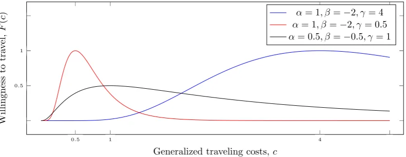
Figure 5: Top-lognormal deterrence functions for different values of parametersα,β andγ.

2.2.3 Top-lognormal deterrence function

A top-lognormal deterrence function is specified by an additional parameterγm>0:

Fm(cijm) =αm·eβmln

2₍cijm

γ )

[image:12.595.93.510.384.545.2]

(13)

ensuring peak attractiveness of a mode is achieved at a target cost interval due to the competitiveness, regulated by theβmparameters, between different modes.

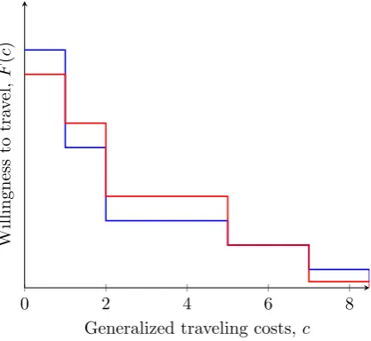
2.2.4 Discrete deterrence function

Another possibility for a deterrence function is the discrete deterrence function. A discrete cost function is specified bync cost bin intervals ¯ck = [ck, ck+1],k= 1, . . . , nc and constant valuesFkmthat the function takes on over these intervals:

Fm(cijm) =       

     

Fm

1 , if cijm ∈¯c1 Fm

2 , if cijm ∈¯c2 ..

.

Fm

nc, if cijm ∈¯cnc

An advantage of using a discrete cost function is that it allows for more flexibility in terms of generating a trip distribution. Too much flexibility can however lead to bad modelling practice. In the real world one expects the willingness to travel to always decrease for increasing travelling costs. As the deterrence function models this willingness to travel one should restrict the choice to monotonically decreasing discrete functions2_. Figure6 shows two examples of such a cost function.

0 2 4 6 8

Generalized traveling costs,c

Willingness

to

tra

v

el,

F

(

c

)

Figure 6: Two discrete distribution functions defined for the same set of cost bins

2.3 Gravity model derivation

In this section we present the mathematical basis for the choice of a gravity model as the trip distribution model. Gravity models have the property that their solution maximizes a quantity called entropy. This was first shown by Wilson[15]. Wilson derives the entropy maximizing property for a unimodal doubly constrained gravity model. Here we apply his approach for the multimodal gravity model described in section2.1that has an exponential cost function (4).

2_{For a unimodal traffic model one can, for the same reason a top-lognormal function is used, allow for unimodal discrete functions}

[image:13.595.196.405.346.538.2]

(14)

The gravity model aims at finding a trip distribution that is the optimum of a certain optimization prob-lem. Namely it aims to find a trip distribution subject to the trip-end constraints (1) and an additional set of cost constraints that maximizes a quantity called entropy. The entropyentropy(T) of a trip distribution T is a measure for the probability of the trip distribution occurring and is defined as:

entropy(T) = _QT! i,j,m

tijm!

WhereT is again the total number of trips modelled. To make the maximization easier we apply Stirling’s approximationln(N!)≈N·ln(N)−N, we instead maximize the following function:

e(T) =−X i,j,m

tijm·ln(tijm)

The additional set of cost constraints is:

X

i,j

tijmcijm=Cm, ∀m

This constraint states that the total amount of capital or budget spent in the region of interest on trips

made by modemis a fixed amountCm. However these constants are assumed to be unknown.

Summarizing, the optimization problem is:

max

T −

X

i,j,m

tijm·ln(tijm) (6)

such that:

X

j,m

tijm=Pi, ∀i (7)

X

i,m

tijm =Aj, ∀j

X

i,j

tijmcijm=Cm, ∀m

We now apply the method of Lagrange multipliers, with multipliersλ(1)_i ,λ(2)_i andβmcorresponding to these constraints, to obtain necessary conditions for local optima:

L=e(T) +X i

λ(1)_i (Pi− X

j,m

tijm)

+X

j

λ(2)_j (Aj− X

i,m

tijm)

+X

m

βm(Cm− X

i,j

tijmcijm)

(15)

∂L(T)

∂tijm

=ln(tijm)−λ

(1)

i −λ

(2)

j −βmcijm, ∀i, j, m This partial derivative should vanish which happens exactly if:

tijm=e−λ

(1)

i −λ

(2)

j −βmcijm_, _∀_{i, j, m}

To obtain the form of the gravity equation (3) we only have to apply two changes in variables:

Oi=e−λ

(1)

i , ∀i

Dj =e−λ

(2)

j _, ∀_j

Giving us:

tijm =OiDje−βmcijm, ∀i, j, m

Note that the partial derivatives of the Lagrangian with respect to the multipliers give us back the con-straints (7).

As the objective function (6) is a concave function and the equality constraints (7) are affine functions the necessary conditions are also sufficient for a local optimum. In fact the concavity of the objective function also implies that any local maximum must be a global maximum as well. It follows that a trip distribution satisfying the gravity equation (3) maximizes entropy.

2.4 Solving the gravity model

2.4.1 OD matrices and skim matrices

Before presenting the solution method to the gravity model we first introduce some convenient matrix notation. It is convenient to think of a trip distribution as a set of matrices, specifically origin-destination matrices (OD matrices) or trip tables. For each modemwe define its OD matrix as the square matrixTm_∈

Rnxn≥0 wheretijm is its (i, j)th entry.

In the same way define generalized cost matricesCm_∈

Rnxn≥0 for each modemwithcijmas the (i, j)thentry of

Cm_{. Generalized costs matrices are also called skim matrices.}

2.4.2 Solution method

The basic doubly constrained simultaneous gravity model described so far can be formulated as:

tijm=OiDjFm(cijm)

X

m,j

tijm=Pi for eachi

X

m,i

tijm=Aj for eachj

(16)

To find a trip distribution that satisfies the gravity model the Furness method is used. In mathematics, the Furness method is better known as IPF (iterative proportional fitting) or matrix raking. The Furness method is described as a series of iterations in which in the odd iterations we scale for each zone the current number of departures towards the target production value and in the even iterations we scale for each zone the current number of arrivals towards the target attraction value. This fitting procedure is started from an initial trip distribution where the trip numbers are equal to the product of the three proportionality factors:

t0_ijm =PiAjFm(cijm) so the starting solution isOi=Pi andDi =Ai for each zonei.

In terms of the OD matricesTmthe method can be described as in the odd iterations scaling the row sums of

the aggregated matrixT =P

mT

m_{towards the target production values}_P

(17)

Algorithm 1Biproportional fitting

1: for eachzoneido

2: Oi←Pi

3: Di←Ai

4: end for

5: for eachmodemdo

6: for eachod pair (i, j)do

7: tijm←Oi·Dj·Fm(cijm)

8: end for

9: end for

10: while not convergeddo

11: for eachzonei do

12: if P

j,mtijm >0 thenf←

Pi

P

j,mtijm

else f ←0

13: Oi←f·Oi

14: for eachzonej do

15: for eachmode mdo

16: tijm←f·tijm

17: end for

18: end for

19: end for

21: if P

i,mtijm>0thenf←

Aj

P

i,mtijm

else f ←0

22: Dj←f·Dj

23: for eachzoneido

24: for eachmode mdo

25: tijm←f·tijm

26: end for

27: end for

28: end for

29: end while

To illustrate the concepts discussed so far we now introduce a simple gravity model instance3 and show how IPF solves it.

Example 2.1. We consider a small instance with two modes and three zones. The production and attraction values for the three zones are assumed to be given by:

P = 

   

80

50

20 

   

, A=h20 30 100

i

Given generalized costs defined by the following skim matrices:

(18)

Ccar =     

5 1 2

1 8 2

1 4 2



   

, Cbike=



   

2 6 3

6 5 5

2 1 4



   

Assuming lognormal deterrence functions with parameters specified by:

(αcar, αbike) = (2,1), and

(βcar, βbike) = (−0.5,−1)

Then the initial trip distribution can be calculated via t0_ijm = PiFm(cijm)Aj (this corresponds with initial balancing factorsOi =Pi andDi=Ai , see algorithm 1):

T_car0 = 

   

642.7 3775 8750.5 1572.9 268.4 5469.1 629.2 328.6 2187.6 

   

, T_bike0 = 

   

64.5 1484.4 2392.9 618.5 12.0 1495.5 247.4 45.0 598.2



   

The first balancing step we scale the rows towards the target production values, this is done by multiplying row factorsf

f =     

0.0047 0.0053 0.0050 

   

to the rows of the OD matrices sucht that the resulting row sums match the production values:

T_car1 = 

   

3.005 17.650 40.914 8.334 1.422 28.979 3.118 1.629 10.841 

   

, T_bike1 = 

   

0.302 6.941 11.188 3.277 0.064 7.924 1.226 0.223 2.964



   

The row factors of f are also multiplied with the production balancing factors to update them:

O=     

0.3740 0.2649 0.0991 

   

The next step consists of scaling the columns towards the target attraction values, we get column factors

f =h1.0383 1.0742 0.9727 i

(19)

T_car2 = 

   

3.120 18.960 39.796 8.654 1.5276 28.187 3.237 1.7493 10.544 

   

, T_bike2 = 

   

0.3133 7.4554 10.882 3.4028 0.0683 7.7077 1.2729 0.2395 2.8834 

   

The attraction balancing factors become:

D=h20.766 32.226 97.267 i

After just two balancing steps the resulting distribution is already matching the trip-ends quite closely. Continuing the balancing process, the distribution would get closer and closer towards the exact solution.

2.4.3 Solution properties and convergence of the biproportional fitting procedure:

Uniqueness

Note that given feasible balancing factors exist, they are not unique. Assuming (O,D) is a solution to the trip end constraints in (8) we clearly have for anyλ >0 that (_λ1·O, λ·D) satisfies the trip-end constraints as well. However given a solution exists the balancing factors are unique up to this constant factor i.e. we only have λ >0 as a degree of freedom. This is proved in theorem2.1. In what follows the balancingfactorsO,D are represented either by a column and row vector orO, D represent diagonal matrices with diagonal entries e.g. Oii =Oi, depending on context.

Theorem 2.1. Uniqueness of trip distribution and balancingfactors.

Let M ∈ Rmxn≥0 be a matrix containing no zero rows or columns. Suppose we have production and

attrac-tion values P ∈ Rm>0, AT ∈ Rn>0. Suppose we have two sets of production and attraction balancing factors

O,O˜∈Rmxm>0 and D,D˜ ∈Rnxn>0 such that both the matrices T =OM D andT˜=OM˜ D˜ satisfy the

produc-tionsP and attractionsA. Then the following two statements hold:

i): The balanced matrices are equal i.e. T =T˜

ii): There exists a constantλ >0 s.t. O˜= 1

λ ·Oand D˜ =λ·D

Proof:

Statement (i) follows directly from theorem 4 in Rothblum[12]. Then with (i) holding (ii) can be proved quite easily: SinceOM D=OM˜ D˜ we must haveOD=O˜D˜ (hereO,O˜represent columns andD,D˜ rows). Then the jth _{columns of these must be equal i.e.} _D

j·O = ˜Dj ·O˜. Since the balancingfactors are positive we can safely takeλ= D˜j

Dj >0. Comparing the i

th_{rows of}_OD₌_O˜_D˜ _{confirms that}_D˜ ₌_λ_·_D_{holds as well for this}

λ.

To apply the theorem to the initial matrix in the biproportional fitting algorithm one should set M =

P

mF

(20)

Existence of solution and convergence of biproportional fitting procedure

In example 2.1 it was shown the biproportional fitting procedure converged for the given instance. An

im-portant question that arises is whether this is the case for every instance. The answer is no as the following counterexample taken from Pukelsheim[11] proves.

Example 2.2. Consider the following unimodal (of one mode) instance with two zones and the following trip-ends: P =   4 2 

, A=

h

2 4

i

Suppose the costs and cost function lead to the initial OD matrix:

T0=   30 0 10 20  

The fact thatt12= 0 could have as an explanation that zone 2 is unreachable from zone 1 which would have been modelled by settingc12 =∞. One can show that the biproportional fitting procedure does not converge in this case but ”oscillates between two distinct accumulation points”[11]:

lim

t=1,3,...T

t₌   4 0 0 2 

, and lim

t=2,4,...T

t₌   2 0 0 4  

Pukelsheim[11] also establishes necessary and sufficient conditions for convergence of the biproportional fitting procedure. His analysis and theorem make use of the so calledL1-error. TheL1-error for the OD matrix in thekthiterationTk denoted byf(k) is calculated by:

f(k) = 1 2 X i X j

tk_ij−Pi +1 2 X j X i

tk_ij−Aj

A column j of the matrixT0 is said to be connected to a row i of that matrix ift0_ij >0. For a subset of rowsI defineJ(I) to be the subset of columns connected toIin the initial OD matrixT0 _i.e. _J₍_I_{) contains all} columns containing a positive entry in some row ofI. Pukelsheim’s main result can now be stated:

Theorem 2.2. Convergence of the biproportional fitting procedure (Pukelsheim[11], 2009)

For an initial matrix T0 _∈

Rmxn≥0 with no zero rows or columns, production and attraction values P ∈ Rm>0,

AT _∈

Rn>0 we have for the limit of theL1-error during the biproportional fitting procedure:

lim

k→∞f(k) =I⊆{max1,...,m}



 X

i∈I

Pi− X

j∈J(I)

Aj 

 (9)

(21)

Again we can simply reduce gravity model instances by eliminating zero rows and columns as well as the rows and columns of zero production and attraction so that the theorem essentially applies to all instances of interest to us.

Some expressions in the maximum of (9) can be computed to possibly detect non-feasibility without

actu-ally running the biproportional fitting procedure. However, for a general instance, theorem2.2 is of little use in proving the biproportional fitting procedure will converge. As determining whether the maximum expres-sion in (9) is greater than zero has a running time of O(2m). Therefore deciding in general whether feasible balancing factors exist is likely best done by just running the biproportional fitting procedure. In this research we found that the fitting procedures converged for each gravity model instance encountered. This suggests that nonconvergence is rare at least in our specific setting.

Purpose

Sub purpose

Mode-user class

Productions

Attractions

combinations

Work

Home

→

Work:

All modes

P

co

_,

_P

nco

_A

Work

→

Home:

All modes

P

A

co

,

A

nco

Business

Home

→

Business:

All modes

P

co

,

P

nco

A

Business

→

Home:

All modes

P

A

co

,

A

nco

Business (home unrelated) - co:

co modes

P

co

A

co

Business (home unrelated) - nco:

nco modes

P

nco

_A

nco

Education

Home

→

Education:

All modes

P

co

_,

_P

nco

_A

Education

→

Home:

All modes

P

A

co

_,

_A

nco

Stores

Home

→

Stores:

All modes

P

co

,

P

nco

A

Stores

→

Home:

All modes

P

A

co

,

A

nco

Other

Home

→

Other - co:

co modes

P

co

A

co

[image:21.595.56.545.304.600.2]

Home

→

Other - nco:

nco modes

P

nco

A

nco

(22)

3 Calibration of the simultaneous gravity model

This chapter gives a detailed explanation of the trip distribution model and the process of calibrating it which is the focus of this thesis. Section3.1first describes the trip distribution model for all purposes and user classes. After that we turn to the main research problem of this thesis, namely the calibration of the gravity model parameters. Section 3.2 discusses within which context the calibration is done and its purpose. Section 3.3

discusses the criteria upon which the calibration process is based. Namely observed trip length distributions and from these derived observed modal splits. Section 3.4 discusses how the modelled counterparts to these observed distributions are calculated. Then section 3.5 first explains the earlier approach to calibrating the lognormal distribution function at Goudappel Coffeng after which a new approach is presented and discussed in section3.6.

3.1 Full trip distribution model

This subsection describes the full trip distribution model used within Goudappel Coffeng which includes user classes and a stratification in trip purposes.

3.1.1 Trip purposes and sub purposes

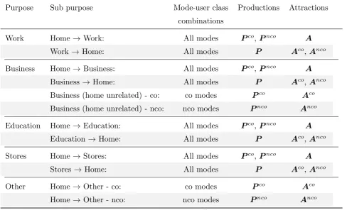
In the real world trips are made for different purposes. For example trips made by people commuting can be labeled with the Work purpose. A trip of a purpose here is further divided into sub purposes which often classify the direction of the trip. In the literature Abdel-Aal[2] also uses purposes in the context of gravity model calibration. The first and second column of table1(page 20) show for the models we will be concerned with the stratification in purposes and sub purposes. Each sub purpose is modelled by a separate gravity model.

3.1.2 User classes

User classes add another dimension to the trip distribution model and add another indexuto the trip number variables: tijmu. Instead of estimating an OD matrixTmfor each modemthe gravity model now estimates an OD matrixTmu_{for each mode-user class pair (}_{m, u}_{). The way in which user classes are exactly embedded into} the gravity model depends on the sub purpose data. We distinguish two cases: In case of symmetric productions and attractions, by which we mean the number of production and attraction values are equal, the sub purpose is simply modelled by the gravity model already encountered. In case of asymmetric productions and attractions the gravity model is extended in an appropriate way. We now discuss these two cases in more detail and in relation to table 1.

Asymmetric productions and attractions

We illustrate the two different gravity models with asymmetric productions and attractions by considering the Work purpose. As shown in table1 the Work purpose has two sub purposes which represent the directions

’Home→Work’ and ’Work→Home’. First we consider the ’Home→Work’ direction. For this direction more

refined data is given regarding its production values: they are distributed over car owners and non car owners, however the attraction side is aggregated. Trips with the ’Home→Work’ direction are modelled by a gravity model of the form:

tijmu=OiuDjFmu(cijm), ∀i, j, m, u s.t.

X

j,m

(23)

X

i,m,u

tijmu=Aj, ∀j (10)

Trips of the reverse ’Work→Home’ direction are modelled by a separate gravity model of the form:

tijmu=OiDjuFmu(cijm), ∀i, j, m, u s.t.

X

j,m,u

tijmu =Pi, ∀i

X

i,m

tijmu =Aju, ∀j, u (11)

The Education and Stores purpose as well as the two sub purposes taken together of the Business purpose are modelled the same way as the Work purpose just described. Each of these have a sub purpose for home based trips, meaning the origins of the trips represent homes while the destinations represent places related to the trips purpose e.g. offices, stores or schools, and each has a reversed direction sub purpose for which the role of origins and destinations are interchanged. The home based sub purpose has distinct production values for both user classes Pco

i , Pinco but single aggregated attraction valuesAj. For the sub purpose of the reverse direction the reverse statement holds.

The solution procedure to these gravity models with asymmetric production and attraction values is described in algorithm 2and is essentially still the biproportional fitting procedure of algorithm 1. In case of user class specific production values we just get double the rows for the aggregate matrixT if we define the OD matrices Tm_{as stacking the matrices}_Tmu _{vertically i.e.}

Tm= 

 Tm,co

Tm,nco





Similarly in case of user class specific attraction values the aggregate matrixT has double the columns with OD matricesTm_{= [}_Tm,co

999T

m,nco_{]. So the problem algorithm}₂ _{solves is still the doubly constrained gravity}

(24)

Algorithm 2Biproportional fitting with user class specific production values and aggregate attraction values for two user classesu∈ {co, nco}

.

1: for eachzoneido 2: Oiu←Piu

3: Di←Ai

4: end for

5: for eachmode-user class pair (m, u)do

7: tijmu←Oiu·Dj·Fmu(cijm)

8: end for

9: end for

12: if P

i,m,utijmu >0 thenf←

Aj

P

i,m,utijm

elsef ←0

13: Dj←f·Dj

14: for eachzoneido

16: tijmu←f·tijmu

17: end for

18: end for

19: end for

20: for eachuser classu∈ {co, nco} do

21: for eachzoneido

22: if P

j,mtijmu>0thenf←

Piu

P

j,mtijmu

elsef ←0

23: Oiu←f ·Oiu

25: for eachmodemdo

26: tijmu←f ·tijmu

27: end for

28: end for

29: end for

30: end for

31: end while

Here the production balancing steps are done last in the while loop. This is done because we are more confident in the accuracy of the production values (as the productions are known separately per user class4_). Balancing the productions last has the result that the production constraints are met exactly. For the same rea-son in the balancing preprocessing step the attraction values should be balanced towards the total of productions.

Symmetric productions and attractions

For the Other purpose only home based trips are modelled. However both user class specific production values and user class specific attraction values are available for these trips and so two doubly constrained gravity

4_{Also because the production data for the sub purposes ’Home}_→_{Work/Business/..’ are more reliable in itself. In the other}

(25)

models are used. One for the car owner user class and one for the non car owner user class. These gravity models are therefore entirely equivalent to the gravity model discussed in chapter 2. For the Business purpose we have two extra sub purposes that model nonhome related trips i.e. business trips for which neither the origin or destination represents a home. Each of these sub purposes models a user class separately similar to the Other purpose.

OD matrix aggregation

We have described how each sub purpose within a trip purpose is modelled by a separate gravity model. However in the rest of this thesis we are interested in the aggregate trip numbers for the trip purposes and so the outcomes of the separate gravity models are aggregated again. Thus for each purpose the OD matricesTmu are equal to the sum of the OD matrices of its respective sub purposes.

3.2 Calibration of deterrence function behavioral parameters

The calibration of the trip distribution model deals with the choice of parameters βmu which appear in the exponential and lognormal cost functions inside the gravity model and additionallyαmu parameters in case of lognormal cost functions. These parameters are called behavioral parameters since they specify behavior of trip makers. The βmu’s model the propensity to make less costly trips for all mode-user class combinations while theαmu’s influence for each user class what percentage of its trip makers use a certain mode of transport i.e. the modal split of the user class. The behavior we try to encapsulate in these parameters is dependent on trip purpose. For example we generally expect trips to school or the shop to be shorter than the commute to work. Therefore the trip distribution model of each purpose is calibrated separately. However the gravity models of the sub purposes that constitute the trip distribution of a purpose share the same set of behavioral parameters. At Goudappel Coffeng the cost function used for the strategic traffic models is usually the lognormal one. The lognormal deterrence function in the case of user classes is of the form:

Fmu(cijm) =αmu·eβmuln

2₍_c

ijm+1) ₍₁₂₎

In this thesis we also assume this lognormal deterrence function so the calibration focuses on both the βmu’s andαmu’s parameters. Note that in (12) the user class index uis omitted incijm as generalized costs are the same for different trip makers.

Transferability of parameters

The production and attractions balancing factors Oi and Dj act upon a subset of cells (rows and columns)

of the OD matrices while the behavioral parameters αmu and βmu act upon the whole matrices. The latter

parameters can be called transferrable parameters. To explain why: suppose we have successfully calibrated the behavioural parameters. The main use of these calibrated behavioural parameters then is to serve as an input for four-step models that consider the same study area but consider different trip-end values or skim matrices in the gravity model. This is done to for example simulate the effect of changes in infrastructure and or zonal characteristics on traffic movement patterns. Changes in infrastructure are modelled by adjusting the road net-work or cost skim matrices and changes in zonal characteristics are modelled by adjusting the socio-economic data which changes the trip-end values of zones.

(26)

3.3 Calibration criteria

The calibration of the behavioral parameters is based on both empirical trip length distributions and modal splits. First we describe what these observed trip length distributions are and how observed modal splits are derived from them. Then we show how the count numbers on which the observed trip length distributions are based can be used to construct confidence intervals.

3.3.1 Empirical trip length distributions and modal splits

For each of the traveling purposes we have for each mode-user class combination (m, u) an empirical trip length distributiondbmuavailable. To obtain such distributions surveys are done for the study area in which respondents were asked to keep a travel diary, for a randomly selected week of the year, in which they keep track of all the trips they made that week. From this data, the number of trips per purpose, mode, user class and distance class was derived and scaled to account for the sampling ratio. In figure7we see, in blue, such a resulting distribution.

[image:26.595.125.471.341.514.2]

From the observed trip length distribution we can, given a user class u, derive for a mode m its observed modal split percentageM Sdmu within that user class by:

Figure 7: An observed (blue) and modelled (red) trip length distribution for the purpose ’Work’, mode car and user class car owners.

d

M Smu=

P

kdbmuk

P ˜

m,kdbmuk˜

Both modelled trip length distributions and modelled modal splits are compared to their observed counter-parts. In section3.4we describe how modelled trip length distributions and modelled modal splits are computed from the OD matrices.

3.3.2 Approximate confidence intervals

(27)

Let N be the total number of counted trips in a survey for some mode-user class combination (m, u). Of these N counts denote bykbi the number of trips with a length in the ith distance bin. Denote bypi the true fraction of trips made with a length in theith_{distance bin. Then for each bin}_k_{the fraction}

b

pi = k_Nbi is a point estimate ofpi. We now provide a measure of the accuracy of these point estimates in the form of approximate confidence intervals for thepk. For more information regarding the construction of binomial confidence intervals we refer to Wallis[14].

From the theory of confidence intervals it follows that an approximate 100(1−α)% - confidence interval forpi is:

pi ∈ "

b

pi−zα/2 r

b

pi(1−p_bi)

N ,pbi+zα/2 r

b

pi(1−p_bi)

N

#

Whereαis the desired significance level andzα/2 is the (1 -α/2)-percentile of the standard normal distri-bution. In caseki= 0 the so called rule of three from statistics can be used which assigns the interval [0,_N3] to

pi. The confidence intervals can be interpreted in the following way: For a significance level ofαwe can expect the constructed intervals to contain the true fraction of trips pi approximately 100(1−α)% of the time. The relative errorri can then be calculated by:

ri=

zα/2 q

b

pi(1−pbi)

N

b

pi

=zα/2 s

1

b

ki − 1

N ≈

zα/2 q

b

ki

, for large N (13)

Thus the width of the confidence intervals is inversely proportional to the square root of the number of observations. The confidence intervals can be plotted as error bars around the observed trip length distribu-tions and form a visual guideline when inspecting the fit of the model to the observed distribudistribu-tions. Another use of these confidence intervals is to incorporate them directly in the objective function by defining weights for the objective function for each distance bin that are inversely proportional to the width of the correspond-ing confidence interval. So in fact these weights are proportional to the square root of the number of observations.

Overestimation of counts

In general there will be a dependency between the trips a survey respondent makes in the same day. The most important dependency is the one resulting from tours i.e. back-and-forth displacements. In the worst case all observations are tours and then the number of observations is overestimated by a factor of 2, leading to an overestimation in confidence by a factor of √2. However the extent to which this is a problem depends upon the time period for which the strategic traffic model is used. For a complete day many tours can be expected to be in the data while one would expect less tours for survey data specific to the morning commute.

3.3.3 Normalization of trip distributions by binwidth

The bins on which the trip distributions are defined are of varying widths. This leads to biased trip length distributions as wider bins are more likely to have more trip counts because a given trip is more likely to fall into a wider bin. To interpret the trip distributions more fairly we can normalize them by bin width. In figure

(28)

[image:28.595.128.467.102.310.2]

Figure 8: Bin width normalized observed (blue) and modelled (red) trip length distribution with confidence bounds (dotted)

3.4 Modelled trip length distributions and modal splits

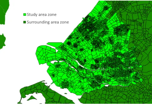
Since in reality the study area is not a closed system in terms of traffic displacements the strategic traffic model also considers zones representing the area surrounding the study-area instead of only those making up the study area. To illustrate this figure9 shows the zonal grid of the study area and surrounding area for the The Hague strategic traffic city model or MRDH model. To save computational effort, generally the size of zones outside the study area increases as the distance to the study area increases.

[image:28.595.270.520.446.619.2]

(a) The Hague city region inside the Netherlands (b) Subdivision of the region into zones

(29)

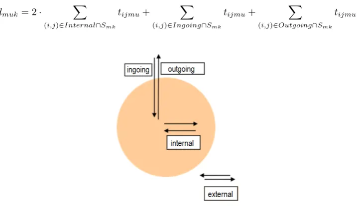
The classification of zones in study-area and surrounding-area zones also brings about a classification in trips. Namely we distinguish study-area related trips which are trips that either start or end in a study area zone and non study-area related or external trips that both start and end in a zone outside the study area. We need to go one step further by partitioning the study-area related trips into internal, ingoing- and outgoing trips for which we use figure10as a definition of these.

The survey counts only include observations of study-area related trips. However these are not counted equally. The number of times a study-area related trip is counted, is equal to the number of times its zone of departure or arrival is a study area zone. So internal trips, in- and outgoing trips, and external trips are counted respectively twice, once and never in the construction of the observed trip length distributions. Now for the purpose of having a fair calibration criterium the modelled trip length distributions (resulting from the gravity models) are computed using the same weights.

Let sijm denote the length of a trip from zone i to zone j made by mode m and the k’s denote length bins (the same bins as those used for the empirical trip length distributions). The zone-to-zone distances logically depend on mode and not on user class. For easier notation in what follows letSmk denote the set of zone-pairs such that the distance between them is in bink, soSmk ={(i, j)|sijm∈sk}. Then the modelled trip length distributiondmuk is given by:

dmuk= 2·

X

(i,j)∈Internal∩Smk

tijmu+

X

(i,j)∈Ingoing∩Smk

tijmu+

X

(i,j)∈Outgoing∩Smk

[image:29.595.120.481.323.530.2]

tijmu

Figure 10: Trips related to the study area: ingoing, outgoing and internal trips versus nonrelated external trips

The modelled modal splits can then be calculated from these trip length distributions by:

M Smu= P

kdmuk

P ˜

m,kdmuk˜

(14)

(30)

Fitting on relative distributions

For the purpose of calibrating theβmu’s we will be interested in approaching the observed relative frequency trip length distributions. The reason for this is that the total number of trips of the observed and modelled trip length distributions are otherwise not necessarily consistent. As during the calibration the proportions of internal, in- and outgoing and external trips are dependent on the current choice of the calibration parameters and these proportions impact the total numbers of trips in the modelled trip length distributions. This normal-ization step makes it so we compare the shapes of the observed and modelled trip length distributions.

Feedback loop

It is perhaps interesting to mention now that usually there is an iterative feedback loop between the trip distri-bution model and the traffic assignment phase in the four-step modelling process. We can imagine costscijmand trip lengthssijm to be arising from the traffic assignment phase as congested traffic routes between zone-pairs would increase the travelling time and possibly eliminate routes. By iterating between the trip distribution and traffic assignment steps the impacts of congestion can be taken into account. This feedback mechanism is however not considered in the calibration as this would be too complicated and too computationally expensive so the calibration is done under static costs and trip lengths.

3.5 Original calibration approach

We now describe the approach that has been used in practice until now at Goudappel Coffeng to automatically calibrate both the α’s and β’s parameters of the lognormal distribution function (12). Fransen[7] devised this approach illustrated in figure 11. It starts with initial parameters α0

[image:30.595.140.453.453.664.2]

mu’s and βmu0 . The initial α0mu’s are first adjusted in an initial change α’s step. Then the algorithm iterates with each iteration consisting of two steps: thechange β’s stepand thechangeα’s step, respectively. The algorithm stops iterating if either a preset maximum number of iterations is reached or the objective function is smaller than a predefined goal value. Next we describe these two steps.

(31)

3.5.1 Change α’s step

The goal of this step is to update theα’s such that the observed modal split is approximately realized. From the gravity equations in (10) and (11) and the lognormal cost function (12) we see that the α’s have a linear influence on the number of trips for each mode. Therefore for each mode-user class pair (m, u) the currentαmu is updated to the newα∗

muby multiplying by a scale factor:

α∗_mu=M Sdmu

M Smu

αmu

WhereM Smu andM Sdmuare again the modelled and observed modal split for mode-user class pair (m, u), respectively.

Then a new modal split M S_mu∗ is computed after running the gravity model with the new α∗’s. This pro-cess is iterated so that new α∗∗’s are determined from the older α∗’s and factors M Sdmu

M S∗

mu until over all the

modes the average relative error between the observed and modelled modal split is smaller than a certain preset percentage.

3.5.2 Change β’s step

A hillclimbing algorithm is used in the old approach to update theβ’s. This original hillclimbing algorithm is described in Fransen[7] and also in section 5.1. Each time a new set of β’s are determined the determination of the α’s (or changeα’s step) that follows has to be done multiple times until the resulting modal split is sufficiently close to the observed modal split. This means that for a single Changeβ’s stepmultiple gravity model runs need to be done (hence the double arrow between the ’Determineα’ and ’Run Gravity Model’ blocks in figure11).

3.6 New calibration approach: modal splits as gravity model constraints

3.6.1 Triproportional fitting procedure

For the following approach we discuss credit is due to Brethouwer[3] who suggested the idea to incorporate the modal split constraints directly into the gravity model when calibrating a lognormal deterrence function. As an example the gravity model for the ’Home→Work’ direction in this new approach is of the form:

tijmu=OiuDjFmu(cijm), ∀i, j, m, u s.t.

X

j,m

tijmu =Piu, ∀i, u

X

i,m,u

tijmu=Aj, ∀j

M Smu=M Sdmu, ∀m, u

(32)

Algorithm 3 Triproportional fitting procedure: balancing respectively towards target attraction, production (user class specific, for two user classesu∈ {co, nco}) and modal split values

.

1: for eachzoneido 2: Oiu←Piu

3: Di←Ai

4: end for

6: αmu←M Sdmu

7: end for

10: tijmu←αmu·Oiu·Dj·Fmu(cijm)

11: end for

12: end for

15: if P

i,m,utijmu >0 thenf←

Aj

P

i,m,utijm

elsef ←0

16: Dj←f·Dj

17: for eachzoneido

19: tijmu←f·tijmu

20: end for

21: end for

22: end for

23: for eachuser classu∈ {co, nco} do

24: for eachzoneido

25: if P

j,mtijmu>0thenf←

Piu

P

j,mtijmu

elsef ←0

26: Oiu←f ·Oiu

28: for eachmodemdo

29: tijmu←f ·tijmu

30: end for

31: end for

32: end for

33: end for

35: Calculate M Smuusing equation (14).

36: if M Smu>0thenf ←

d

M Smu

elsef ←0

37: αmu←f ·αmu

39: tijmu=f·tijmu

40: end for

41: end for

(33)

The advantage of this new approach is that it requires only a method to calibrate theβmu’s parameter set, as the αmu’s are now a function of the βmu’s. In the original calibration approachαmu’s are arrived at only after multiple changeα’ssteps in between the change β’ssteps. The new calibration approach only requires about 20% of the running time of the old calibration approach and achieves the target modal splits exactly.

3.6.2 Discussion: Comparison with old approach

Convergence of the triproportional fitting procedure is like the biproportional fitting procedure not guaranteed but in this research we observed convergence for each of the encountered problem instances. It was also observed that the triproportional fitting procedure converges to the same trip distribution as the biproportional fitting procedure i.e. algorithm 2 for which the lognormal parameters are initially set to the modal split balancing factors obtained in the triproportional fitting procedure. This is also predicted by theorem2.1. For example, in case of user specific production values, setM in the theorem according to:

M =X m





Fm,co₍_Cm,co_{, α}

m,co)

Fm,nco₍_Cm,nco_{, α}

m,nco)





Assuming both procedures converged i.e. balancing factors Obi,Dbi and Otri,Dtri were found such that the converged aggregated OD matricesTbi =ObiM Dbi andTtri=OtriM Dtrisatisfy the productions and attrac-tions. Then by theorem2.1 these aggregated OD matrices are equal i.e. Tbi =Ttri and the balancing factors

Obi,Dbi andOtri,Dtriare equal up to constant scaling. Then clearly the disaggregate OD matrices per mode and user class must be the same too.

The importance of these distributions being equal is that the nature of the biproportional gravity model is still intact with the extra balancing step. The modal split balancing step gives a trip distribution satisfying modal split while still maximizing entropy subject to the trip end constraints for the chosenβmuand (resulting)

αmu. The αmu’s resulting from the triproportional procedure can therefore still be interpreted as behavioral parameters of the lognormal deterrence function and are still transferable between different models.

3.6.3 Modal split aggregateness

(34)

4 Mathematical problem formulation

In this section we give the mathematical problem formulation that we will focus on solving. Specifically we formulate the new triproportional calibration approach discussed in section 3.6as a bilevel optimization prob-lem. Section4.1 discusses some potential choices for the calibration objective function after which in section

4.2 the bilevel problem is formulated. Section4.3 gives the convergence criterion used for the gravity models and explains its importance. Finally section 4.4gives a list of performance criteria to be taken in mind in the search for potential solution methods.

Some notation:

We first introduce some vector notation for some of the already encountered variables of the trip distribution

model. Denote by β the full set of parametersβmu of the trip purpose being calibrated at hand. Remember

that within a purpose the parameter set of each sub purpose is this set (or a proper subset of this set as logically a user class specific sub purpose inherits only the parameters of its user class). Denote byO,D,αthe full set of production, attraction and modal split balancing factors that relate to the purpose. So each of these sets are the union of the subsets of balancing factors resulting from the IPF procedures for the different sub purpose gravity models. Similarly here byT we denote a full purpose trip distribution i.e. the set of all (disaggregated) trip numberstijmu related to the sub purposes of a specific purpose.

4.1 Calibration objective function

In section 3.4 we showed how to derive the modelled trip length distribution from a trip distribution. In the calibration one wants to choose parametersβmusuch that the modelled trip length distributions in some sense approach the observed trip length distributions. An objective function that is useful to measure the similarity between two distributions is to take the sum of squared differences:

F(β) = X

m,u,k

(d_mukrel −db_mukrel )2 (15)

Here d_mukrel and db_mukrel represent respectively modelled and observed relative trip length distributions both expressed in percentages. They can be calculated by:

d_mukrel = 100· _Pdmuk

k0dmuk0

! (%)

b

d_mukrel = 100· dbmuk

P

k0db_muk0

! (%)

The relative numbers are preferred in (15) since the total number of modelled trips can vary during the calibration as reasoned in section 3.4. The trip length distribution numbers dmuk anddbmuk can either denote absolute trip numbers or these normalized by distance bin width as described in section 3.3.3. Note that the objective function in (15) is written as a function of the parameter set β because the modelled trip length distributions are a function of this parameter set. This fact will be made more clear in the next section. If one is more interested in mileage than trip numbers one can apply a weighting resulting in the following objective function:

F(β) = X

m,u,k

(35)

Here the bin midpointsmk serve as weights with the goal of better fitting on distance bins of higher length. A reason it can be desirable to better fit in this way on the total amount of mobility measured in mileage is due to the trip assignment phase of the four step model. OD pairs further apart have longer routes in the road network which naturally then consist of more links compared to routes of shorter distanced OD pairs. The resulting link flows of the trip assignment phase is compared based on a subset of links that have observed traffic counts attached to them. Since the trip numbers of the higher distance bins impact more links, and so likely more links with counts attached, a better fit in the trip distribution phase likely translates to a better general fit in the trip assignment phase.

Another alternative objective function is:

F(β) =X m,u

(1−r2mu)

withrmubeing the Pearson correlation coefficient between the (absolute) observed and modelled trip length distributions. This objective function was used for the original calibration approach before this research. The correlation coefficient is invariant to scaling of the series and therefore automatically compares relative distribu-tions. However we have chosen to use the objective function of equation (15) as it is easier to find the derivative of it as well as the measure itself is easier to explain.

4.2 Bilevel optimization problem

This subsection gives an mathematical optimization problem formulation for the problem of calibrating a trip distribution model of a trip purpose. The optimization problem is of a special kind. Namely it is a bilevel optimization problem where the problem of maximizing entropy or solving the gravity model is embedded within the calibration of the gravity model parametersβ. We refer to solving the gravity model as the inner optimization problem and the problem of selecting the optimalβduring the calibration as the outer optimization problem.

The bilevel optimization problem is then formulated as:

min

β<0,(O,D,α)≥0F(β,O,D,α) s.t. : (16)

(O,D,α)∈ arg max (O˜,D˜,α˜)≥0

{entropy(T)|T =T(β,O˜,D˜,α˜) satisfies the relevant trip end and modal split constraints}

The solution method for the inner optimization problem is the triproportional fitting procedure of algorithm

(36)

IPF procedure Calculate objective function

objective function value,

F(β)

modelled trip length distributions,

d

β

observed trip length distributions,

d̂ balancing factors O, D, α

[image:36.595.122.474.96.217.2]

Trip-end constraints sufﬁciently satisﬁed ?

Figure 12: Flowchart of the bilevel optimization problem

4.3 Gravity model convergence criterion

Assuming the IPF-procedures converges, its solution is still inexact, meaning generally there will be some residual in the trip end constraints after any finite number of IPF iterations. Therefore a gravity model convergence criterion (the diamond shaped box in figure12) needs to be established. The choice of a threshold used in the convergence criterion will have an impact on the bilevel optimization problem as these determine the number of IPF iterations required which naturally impacts the balancing factors and objective function. It does not make much sense to base the convergence criterion on absolute residual errors as different strategic traffic models give rise to different orders of absolute trip numbers. Therefore the convergence criterion we will be using is based

on relative residuals. For example in the case of the gravity model for the ’Home→ Work’ sub purpose the

maximum relative residuals of production and attraction constraints respectivelyRrel

prodandRrelattr as defined by:

Rrel_prod= max i,u

(P

j,mtijmu−Piu)

Piu

(17)

Rrel_attr= max j

(P

i,m,utijmu−Aj)

Aj

The convergence criterion is then to enforce that both of these maximum relative residuals should be smaller than a preset percentage. Note that the modal split constraints do not need to be included in the convergence criterion as they are satisfied exactly as the IPF procedure terminates on a modal split balancing step, see algorithm 3. Indeed a different order could be chosen putting e.g. the production and attraction balancing steps last which would imply the production and attraction constraints are deemed more important than the modal split constraints. However it was observed in this research that the order favoring modal split constraints was only behind at most 1-2 iterations in terms of convergence in Rrel

prod and Rrelattr, suggesting the order we choose only matters slightly.

Gravity model parameter calibration for large scale strategic transport models