University of Warwick institutional repository: http://go.warwick.ac.uk/wrap
This paper is made available online in accordance with
publisher policies. Please scroll down to view the document
itself. Please refer to the repository record for this item and our
policy information available from the repository home page for
further information.
To see the final version of this paper please visit the publisher’s website.
Access to the published version may require a subscription.
Author(s): Louigi Addario-Berry, Nicolas Broutin and Christina
Goldschmidt
Article Title: Critical random graphs: limiting constructions and
distributional properties
Year of publication: 2010
Link to published article:
El e c t ro n ic
Jo ur
n a l o
f P
r o
b a b il i t y
Vol. 15 (2010), Paper no. 25, pages 741–775. Journal URL
http://www.math.washington.edu/~ejpecp/
Critical random graphs: limiting constructions and
distributional properties
∗
†
L. Addario-Berry
Department of Mathematics and Statistics McGill University 805 Sherbrooke W. Montréal, QC, H3A 2K6, Canada
N. Broutin
Projet Algorithms INRIA Rocquencourt
78153 Le Chesnay France
C. Goldschmidt
Department of Statistics University of Warwick Coventry CV4 7AL UK
Abstract
We consider the Erd˝os–Rényi random graph G(n,p) inside the critical window, where p = 1/n+λn−4/3for some λ∈R. We proved in [1]that considering the connected components
ofG(n,p)as a sequence of metric spaces with the graph distance rescaled byn−1/3and letting n→ ∞yields a non-trivial sequence of limit metric spacesC = (C1,C2, . . .). These limit metric spaces can be constructed from certain random real trees with vertex-identifications. For a single such metric space, we give here two equivalent constructions, both of which are in terms of more standard probabilistic objects. The first is a global construction using Dirichlet random variables and Aldous’ Brownian continuum random tree. The second is a recursive construction from an inhomogeneous Poisson point process onR+. These constructions allow us to characterize the
distributions of the masses and lengths in the constituent parts of a limit component when it is decomposed according to its cycle structure. In particular, this strengthens results of Łuczak et al.[29]by providing precise distributional convergence for the lengths of paths between ker-nel vertices and the length of a shortest cycle, within any fixed limit component.
∗MSC 2000 subject classifications: primary 05C80; secondary 60C05.
†L.A.B. was supported by an NSERC Discovery Grant throughout the research and writing of this paper. C.G. was
Key words: random graph; real tree; scaling limit; Gromov–Hausdorff distance; Brownian ex-cursion; continuum random tree; Poisson process; urn model.
1
Introduction
TheErd˝os–Rényi random graph G(n,p)is the random graph on vertex set{1, 2, . . . ,n}in which each of the n2
possible edges is present independently of the others with probabilityp. In the 50 years since its introduction [20], this simple model has given rise to a very rich body of mathematics. (See the books[14, 26]for a small sample of this corpus.) In a previous paper[1], we considered therescaled global structureofG(n,p)forpin thecritical window– that is, wherep=1/n+λn−4/3 for someλ ∈R – when individual components are viewed as metric spaces with the usual graph
distance. (See [1] for a discussion of the significance of the random graph phase transition and the critical window.) The subject of the present paper is the asymptotic behavior of individual components ofG(n,p), again viewed as metric spaces, when pis in the critical window.
LetC1n,C2n, . . . be the connected components of G(n,p)listed in decreasing order of size, with ties broken arbitrarily. Write Cn = (C1n,C2n, . . .)and write n−1/3Cn to mean the sequence of compo-nents viewed as metric spaces with the graph distance in each multiplied byn−1/3. Let dGH be the Gromov–Hausdorff distance between two compact metric spaces (see[1]for a definition).
Theorem 1([1]). There exists a random sequenceC of compact metric spaces such that as n→ ∞,
n−1/3Cn d→ C,
where the convergence is in distribution in the distance d specified by
d(A,B) = ∞ X
i=1
dGH(Ai,Bi)4 !1/4
.
We refer to the individual metric spaces in the sequence C as the componentsofC. The proof of Theorem 1 relies on a decomposition of any connected labeled graphG into two parts: a “canoni-cal” spanning tree (see[1]for a precise definition of this tree), and a collection of additional edges which we callsurplus edges. Correspondingly, the limiting sequence of metric spaces has a surpris-ingly simple description as a collection of random real trees (given below) in which certain pairs of vertices have been identified (vertex-identification being the natural analog of adding a surplus edge, since edge-lengths are converging to 0 in the limit).
In this paper, we consider the structure of the individual components of the limitC in greater detail. In the limit, these components have a scaling property which means that, in order to describe the distributional structure of a component, only the number of vertex identifications (which we also call the surplus) matters, and not the total mass of the tree in which the identifications take place. The major contribution of this paper is the description and justification of two construction procedures for building the components ofC directly, conditional on their size and surplus. The importance of these new procedures is that instead of relying on a decomposition of a component into a spanning tree and surplus, they rely on a decomposition according to the cycle structure, which from many points of view is much more natural.
the kernel. (However, we do not spell out the details of the finite construction since it does not lead to any further results.) It is this procedure that yields the strengthening of the results of Łuczak, Pittel, and Wierman[29].
The second procedure contains Aldous’ stick-breaking inhomogeneous Poisson process construction of the Brownian CRT as a special case. Aldous’ construction, first described in[2], has seen nu-merous extensions and applications, among which the papers of Aldous[5], Aldous, Miermont, and Pitman[8], Peres and Revelle[30], Schweinsberg[34]are notable. In particular, in the same way that the Brownian CRT arises as the limit of the uniform spanning tree in ofZd ford ≥4 (proved
in [34]), we expect our generalization to arise as the scaling limit of the components of critical percolation inZd or thed-dimensional torus, for larged.
Before we move on to the precise description of the constructions, we introduce them informally and discuss their relationship with various facts about random graphs and the Brownian continuum random tree.
1.1
Overview of the results
A key object in this paper is Aldous’ Brownian continuum random tree (CRT)[2–4]. In Section 2, we will give a full definition of the Brownian CRT in the context ofreal trees coded by excursions. For the moment, however, we will simply note that the Brownian CRT is encoded by a standard Brownian excursion, and give a more readily understood definition using a construction given in[3].
STICK-BREAKING CONSTRUCTION OF THEBROWNIAN CRT. Consider an inhomogeneous Poisson process on R+ with instantaneous rate t at t ∈ R+. Let J1,J2, . . . be its inter-jump times, in the order they occur (J1 being measured from 0). Now construct a tree as follows. First take a (closed) line-segment of lengthJ1. Then attach another line-segment of length J2 to a uniform position on the first line-segment. Attach subsequent line-segments at uniform positions on the whole of the structure already created. Finally, take the closure of the object obtained.
The canonical spanning tree appearing in the definition of a component ofC is not the Brownian CRT, except when the surplus is 0; in general, its distribution is defined instead as a modification (via a change of measure) of the distribution of the Brownian CRT which favors trees encoded by excursions with a large area (see Section 2 for details). We refer to such a continuum random tree as atiltedtree. One of the main points of the present work is to establish strong similarity relationships between tilted trees and the Brownian CRT which go far beyond the change of measure in the definition.
Our first construction focuses on acombinatorialdecomposition of a connected graph into its cycle structure (kernel) and the collection of trees obtained by breaking down the component at the vertices of the kernel. In the case of interest here, the trees are randomly rescaled instances of Aldous’ Brownian CRT. This is the first direct link between the components of C having strictly positive surplus and the Brownian CRT.
in the first lengths does not, in general, give a consistent construction: if the distribution is not exactly right, then the initial, biased lengths will appear too short or too long in comparison to the intervals created by the Poisson process. Indeed, it was nota prioriobvious to the authors that such a distribution must necessarily exist. The consistency of this construction is far from obvious and a fair part of this paper is devoted to proving it. In particular, the results we obtain for the combinatorial construction (kernel/trees) identify the correct distributions for the first lengths. Note in passing that the construction shows that the change of measure in the definition of tilted trees is entirely accounted for by biasing a (random) number of paths in the tree.
The first few lengths mentioned above are the distances between vertices of the kernel of the com-ponent. One can then see the stick-breaking construction as jointly building the trees: each interval chooses a partially-formed tree with probability proportional to the sum of its lengths (the current mass), and then chooses a uniformly random point of attachment in that tree. We show that one can analyze this procedure precisely via a continuous urn process where the bins are the partial trees, each starting initially with one of the first lengths mentioned above. The biased distribution of the initial lengths in the bins ensures that the process builds trees in the combinatorial construction which are not only Brownian CRT’s but also have the correct joint distribution of masses. The proof relies on a decoupling argument related to de Finetti’s theorem[9, 16].
1.2
Plan of the paper
The two constructions we have just informally introduced are discussed precisely in Section 2. Along the way, Section 2 also introduces many of the key concepts and definitions of the paper. The distributional results are stated in Section 3. The remainder of the document is devoted to proofs. In Section 4 we derive the distributions of the lengths in a component ofC between vertices of the kernel. The stick-breaking construction of a component ofC is then justified in Section 5. Finally, our results about the distributions of masses and lengths of the collection of trees obtained when breaking down the cycle structure at its vertices are proved in Section 6.
2
Two constructions
Suppose that Gmp is a (connected) component of G(n,p) conditioned to have size (number of
ver-tices) m≤ n. Theorem 1 entails that Gmp, with mn−2/3 →σand pn→1 as n→ ∞and distances rescaled byn−1/3, converges in distribution to some limiting metric space, in the Gromov–Hausdorff sense. (We shall see that the scaling property mentioned above means in particular that it will suffice to consider the caseσ= 1.) We refer to this limiting metric space as “a component ofC, conditioned to have total sizeσ”. From the description as a finite graph limit, it is clear that this distribution should not depend upon where in the sequenceC the component appears, a fact we can also obtain by direct consideration of the limiting object (see below).
2.1
The viewpoint of Theorem 1: vertex identifications within a tilted tree.
presentation in this section owes much to the excellent survey paper of Le Gall[28]. Areal treeis a compact metric space(T,d)such that for allx,y∈ T,
• there exists a unique geodesic from x to y i.e. there exists a unique isometry fx,y : [0,d(x,y)]→ T such that fx,y(0) = x and fx,y(d(x,y)) = y. The image of fx,y is called
¹x,yº;
• the only non-self-intersecting path from x to y is¹x,yºi.e. ifq:[0, 1]→ T is continuous and injective and such thatq(0) =x andq(1) = y thenq([0, 1]) =¹x,yº.
In practice, the picture to have in mind is of a collection of line-segments joined together to make a tree shape, with the caveat that there is nothing in the definition which prevents “exotic behavior” such as infinitary branch-points or uncountable numbers of leaves (i.e. elements of T of degree 1). Real trees encoded by excursions are the building blocks of the metric spaces with which we will deal in this paper, and we now explain them in detail. By anexcursion, we mean a continuous functionh:[0,∞)→R+ such thath(0) =0, there existsσ <∞such thath(x) =0 for x > σand
h(x)>0 for x∈(0,σ). Define a distancedh on[0,∞)via
dh(x,y) =h(x) +h(y)−2 inf
x∧y≤z≤x∨yh(z)
and use it to define an equivalence relation: take x ∼ y if dh(x,y) =0. Then the quotient space Th:= [0,σ]/∼endowed with the distancedhturns out to be a real tree. We will always think ofTh
as being rooted at the equivalence class of 0. Whenhis random, we callTha random real tree. The excursionhis often referred to as theheight processof the treeTh. We note thatThcomes equipped with a naturalmass measure, which is the measure induced onThfrom Lebesgue measure on[0,σ]. By a real tree ofmassorsizeσ, we mean a real tree built from an excursion of lengthσ.
Aldous’Brownian continuum random tree (CRT)[2–4]is the real tree obtained by the above proce-dure when we takeh=2e, wheree= (e(x), 0≤x ≤1)is a standard Brownian excursion.
The limitC = (C1,C2, . . .) is a sequence of compact metric spaces constructed as follows. First, take a standard Brownian motion (W(t),t ≥ 0) and use it to define the processes(Wλ(t),t ≥0) and(Bλ(t),t≥0)via
Wλ(t) =W(t) +λt− t
2
2, and B
λ(t) =Wλ(t)− min
0≤s≤tW λ(s).
Now take a Poisson point process inR+×R+ with intensity 12L2, where L2 is Lebesgue measure in the plane. The excursions of 2Bλ away from zero correspond to the limiting components ofC: each excursion encodes a random real tree which “spans” its component, and the Poisson points which fall under the process (and, in particular, under specific excursions) tell us where to make vertex-identifications in these trees in order to obtain the components themselves. We next explain this vertex identification rule in detail.
For a given excursionh, letAh={(x,y): 0≤x≤σ, 0≤ y ≤h(x)}be the set of points underhand above thex-axis. Let
be the points of [0,σ] nearest to x for which h(`(ξ)) = h(r(ξ)) = y (see Figure 1). It is now straightforward to describe how the points of a finite pointsetQ ⊆Ahcan be used to make
vertex-identifications: forξ∈ Q, we simply identify the equivalence classes[x]and[r(x)]inTh. (It should always be clear that the points we are dealing with in the metric spaces are equivalence classes, and we hereafter drop the square brackets.) We writeg(h,Q)for the resulting “glued” metric space; the tree metric is altered in the obvious way to accommodate the vertex identifications.
To obtain the metric spaces in the sequenceC from 2Bλ, we simply make the vertex identifications induced by the points of the Poisson point process in R+×R+ which fall below 2Bλ, and then
rearrange the whole sequence in decreasing order of size. The reader may be somewhat puzzled by the fact that we multiply the processBλ by 2 and take a Poisson point process of rate 12. It would seem more intuitively natural to use the excursions of Bλ and a Poisson point process of unit rate. However, the lengths in the resulting metric spaces would then be too small by a factor of 2. This is intimately related to the appearance of the factor 2 in the height process of the Brownian CRT. Further discussion is outside the purview of this paper, but may be found in[1].
x r(x)
[image:8.612.189.428.295.431.2]ξ
Figure 1: A finite excursionhon[0, 1]coding a compact real treeTh. Horizontal lines connect points of the
excursion which form equivalence classes in the tree. The pointξ= (x,y)yields the identification of the equivalence classes[x]and[r(x)], which are represented by the horizontal dashed lines.
Above, we have described a way of constructing thesequence of metric spacesC. In order to see what this implies about a single component of C, we must first explain the scaling property of the componentsCkmentioned above. First, consider the excursions above 0 of the processBλ. An excursion theory calculation (see[1, 6]) shows that, conditional on their lengths, the distributions of these excursions do not depend on their starting points. Write ˜e(σ)for such an excursion conditioned to have lengthσ; in the caseσ=1, we will simply write ˜e. The distribution of ˜e(σ) is most easily described via a change of measure with respect to the distribution of a Brownian excursion e(σ) conditioned to have lengthσ: for any test function f,
E[f(˜e(σ))] = E
h
f(e(σ))expRσ 0 e
(σ)(x)d xi
E
h
expRσ
0 e(σ)(x)d x
i . (1)
under the excursion 2˜e(σ). Note that as a consequence of the homogeneity ofP, conditional on ˜
e(σ), the number of points|P |has a Poisson distribution with meanRσ 0 ˜e
(σ)(x)d x.
Lete(σ)(·) =pσe(·/σ)as above. Then for any test function f, by the tower law for conditional expectations we have
E
f(˜e(σ))| |P |=k=E
f(e˜(σ))1{|P |=k}
P(|P |=k)
=E
E
f(˜e(σ))1{|P |=k}|˜e(σ)
E
P
|P |=k|e˜(σ)
=E h
f(˜e(σ))·k1! R0σ˜e(σ)(u)duk
exp −R0σ˜e(σ)(u)dui
E
h 1
k! Rσ
0 ˜e(u)du k
exp −R0σ˜e(σ)(u)dui
=E h
f(e(σ))· Rσ 0 e
(σ)(u)duki
E
h Rσ
0 e(σ)(u)du ki
=E h
f(pσe(·/σ)) R1
0 e(u)du ki
E
h R1
0 e(u)du ki
.
Thus, conditional on|P |=k, the behavior of the tilted excursion of lengthσmay be recovered from that of a tilted excursion of length 1 by a simple rescaling. Throughout the paper, in all calculations that are conditional on the number of Poisson points|P |, we will takeσ=1 to simplify notation, and appeal to the preceding calculation to recover the behavior for other values ofσ.
Finally, suppose that the excursions of Bλ have ordered lengths Z1 ≥ Z2 ≥ . . . ≥ 0. Then condi-tional on their sizes Z1,Z2, . . . respectively, the metric spacesC1,C2, . . . are independent and Ck is distributed as g(2˜e(Zk),P), k≥ 1. It follows that one may construct an object distributed as a
component ofC conditioned to have sizeσas follows.
VERTEX IDENTIFICATIONS WITHIN A TILTED TREE
1. Sample a tilted excursion ˜e(σ).
2. Sample a set P containing a PoissonR0σ˜e(σ)(x)d x number of points
uni-form in the area under 2˜e(σ).
3. Outputg(2˜e(σ),P).
The validity of this method is immediate from Theorem 1 and from (1).
2.2
Randomly rescaled Brownian CRT’s, glued along the edges of a random kernel.
Graphs and their cycle structure. The number of surplus edges, or simplysurplus, of a connected labeled graphG= (V,E)is defined to bes=s(G) =|E| − |V|+1. In particular, trees have surplus 0. We say that the connected graph G is unicylic if s = 1, and complex if s ≥ 2. Define the core (sometimes called the 2-core) C = C(G) to be the maximum induced subgraph of G which has minimum degree two (so that, in particular, if G is a tree then C is empty). Clearly the graph induced byG on the set of vertices V\V(C)is a forest. So ifu∈V \V(C), then there is a unique shortest path inG fromuto some v∈V(C), and we denote thisv byc(u). We extend the function c(·)to the rest ofV by settingc(v) =vforv∈V(C).
We next define thekernel K=K(G)to be the multigraph obtained fromC(G)by replacing all paths whose internal vertices all have degree two inC and whose endpoints have degree at least three in C by a single edge (see e.g. [26]). If the surplussis at most 1, we agree that the kernel is empty; otherwise the kernel has minimum degree three and precisely s−1 more edges than vertices. It follows that the kernel always has at most 2svertices and at most 3sedges. We write mult(e)for the number of copies of an edgeein K. We now defineκ(v)to be “the closest bit ofK tov”, whether that bit happens to be an edge or a vertex. Formally, ifv∈V(K)we setκ(v) =v. Ifv∈V(C)\V(K) then v lies in a path in G that was contracted to become some copy ek of an edge ein K; we set κ(v) =ek. If v∈V(G)\V(C)then we set κ(v) = κ(c(v)). In this last case, κ(v)may be an edge or a vertex, depending on whether or not c(v) is in V(K). The graphs induced by G on the sets
κ−1(v)or κ−1(e
k) for a vertex v or an edge ek of the kernelK are trees; we call themvertex trees
andedge trees, respectively, and denote them T(v)and T(ek). It will always be clear from context to which graph they correspond. In each copyekof an edgeuv, we distinguish inT(ek)the vertices that are adjacent touand von the unique path fromutov in the coreC(G), and thus view T(ek) as doubly-rooted.
Before we define the corresponding notions of core and kernel for the limit of a connected graph, it is instructive to discuss the description of a finite connected graphG given in[1](and alluded to just after Theorem 1), and to see how the core appears in that picture. LetG= (V,E)be connected and with ordered vertex set; without loss of generality, we may suppose that thatV = [m]for some m ≥ 1. Let T = T(G) be the so-calleddepth-first tree. This is a spanning tree of the component which is derived using a certain “canonical” version of depth-first search. (Since the exact nature of that procedure is not important here, we refer the interested reader to[1].) LetE∗=E\E(T)be the set of surplus edges which must be added to T in order to obtainG. LetV∗be the set of endpoints of edges in E∗, and let TC(G) be the union of all shortest paths in T(G)between elements of V∗. Then the coreC(G)is preciselyTC(G), together with all edges inE∗, andTC(G) =T(C(G)).
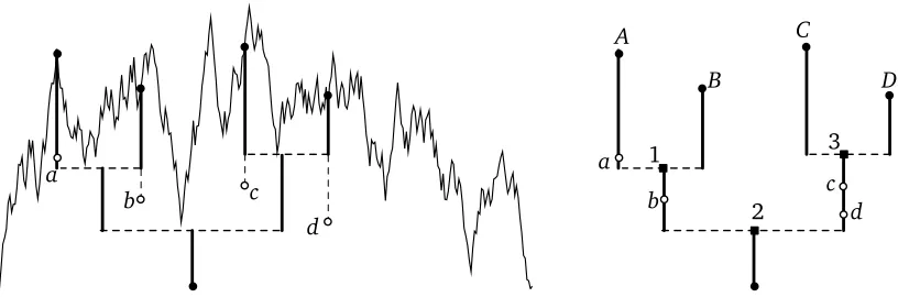
The cycle structure of sparse continuous metric spaces. Now consider a real treeThderived from an excursionh, along with a finite pointsetQ ⊆Ah which specifies certain vertex-identifications, as
described in the previous section. LetQx ={x :ξ= (x,y)∈ Q}and letQr={r(x):ξ= (x,y)∈ Q}, both viewed as sets of points of Th. We let TC(h,Q) be the union of all shortest paths inTh
between vertices in the setQx∪ Qr. ThenTC(h,Q)is a subtree ofTh, with at most 2|Q|leaves (this
is essentially the pre-coreof Section 4.2). We define the core C(h,Q) of g(h,Q) to be the metric space obtained from TC(h,Q) by identifying x and r(x) for eachξ= (x,y)∈ Q. We obtain the kernel K(h,Q)from the coreC(h,Q)by replacing each maximal path inC(h,Q)for which all points but the endpoints have degree two by an edge. For an edgeuvofK(h,Q), we writeπ(uv)for the path inC(h,Q)corresponding touv, and|π(uv)|for its length.
For each x, let c(x) be the nearest point of TC(h,Q) to x in Th. In other words, c(x)is the point
analogous way to the definition for finite graphs. For a vertexvofK(h,Q), we define thevertex tree T(v)to be the subgraph of g(h,Q)induced by the points inκ−1(v) ={x :c(x) =v}and the mass
µ(v)as the Lebesgue measure ofκ−1(v). Similarly, for an edgeuvof the kernelK(h,Q)we define theedge tree T(uv)to be the tree induced byκ−1(uv) ={x :c(x)∈π(uv),c(x)6=u,c(x)6=v}∪{u,v}
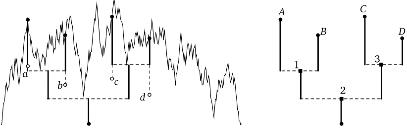
and writeµ(uv) for the Lebesgue measure ofκ−1(uv). The two pointsuand v are considered as distinguished in T(uv), and so we again view T(uv) as doubly-rooted. It is easily seen that these sets are countable unions of intervals, so their measures are well-defined. Figures 2 and 3 illustrate the above definitions.
a
b c
d
A
B
C
D
1
2
[image:11.612.92.503.203.335.2]3
Figure 2: An excursionhand thereduced treewhich is the subtreeTR(h,Q)ofThspanned by the root and the
leavesA,B,C,Dcorresponding to the pointsetQ={a,b,c,d}(which has sizek=4). The tree TR(h,Q)is a
combinatorial tree with edge-lengths. It will be important in Section 4 below. It has 2kvertices: the root, the leaves and the branch-points 1, 2, 3. The dashed lines have zero length.
A
B
C
D
a
b c
d
1 3
A
B
C
D
a
b c
d
1 3
a 1
b d
3 c
Figure 3: From left to right: the treeTC(h,Q)from the excursion and pointset of Figure 2, the corresponding
kernelK(h,Q)and coreC(h,Q). The dashed lines indicate vertex identifications.
Sampling a limit connected component. There are two key facts for the first construction pro-cedure. The first is that, for a random metric space g(2˜e,P) as above, conditioned on its mass, an edge tree T(uv) is distributed as a Brownian CRT of mass µ(uv) and the vertex trees are al-most surely empty. The second is that the kernel K(2˜e,P) is almost surely 3-regular (and so has
2(|P | −1)vertices and 3(|P | −1)edges). Furthermore, for any 3-regularK witht loops,
P(K(2˜e,P) =K | |P |)∝
2t Y
e∈E(K)
mult(e)! −1
. (2)
[image:11.612.80.501.407.512.2]limit version of a special case of [25, Theorem 7 and (1.1)], and is alluded to in[26], page 128, and so is also unsurprising.) These two facts, together with some additional arguments, will justify the validity of our first procedure for building a component ofC conditioned to have sizeσ, which we now describe.
Let us condition on|P |=k. As explained before, it then suffices to describe the construction of a component of standard massσ=1.
PROCEDURE1: RANDOMLY RESCALEDBROWNIANCRT’S
• Ifk=0 then let the component simply be a Brownian CRT of total mass 1.
• If k = 1 then let (X1,X2) be a Dirichlet(1 2,
1
2) random vector, let T1,T2 be independent Brownian CRT’s of sizes X1 and X2, and identify the root of T1 with a uniform leaf ofT1and with the root ofT2, to make a “lollipop” shape.
• Ifk≥2 then letK be a random 3-regular graph with 2(k−1)vertices chosen according to the probability measure in (2), above.
1. Order the edges ofK arbitrarily ase1, . . . ,e3(k−1), withei=uivi.
2. Let (X1, . . . ,X3(k−1))be a Dirichlet(12, . . . , 1
2)random vector (see Section 3.1 for a definition).
3. Let T1, . . . ,T3(k−1) be independent Brownian CRT’s, with treeTi having massXi, and for eachiletri andsi be the root and a uniform leaf ofTi.
4. Form the component by replacing edge uivi with treeTi, identifying ri withui andsi withvi, fori=1, . . . , 3(k−1).
In this description, as in the next, the cases k = 0 and k = 1 seem inherently different from the cases k≥ 2. In particular, the lollipop shape in the case k=1 is a kind of “rooted core” that will arise again below. For this construction technique, the use of a rooted core seems to be inevitable as our methods require us to work with doubly rooted trees. Also, as can be seen from the above description, doubly rooted trees are natural objects in the context of a kernel. However, they seem more artificial for graphs whose kernel is empty. Finally, we shall see that the use of a rooted core also seems necessary for the second construction technique in the case k=1, a fact which is more mysterious to the authors.
An aside: the forest floor picture. It is perhaps interesting to pause in order to discuss a rather different perspective on real trees with vertex identifications. Suppose first that T is a Brownian CRT. Then the path from the root to a uniformly-chosen leaf has a Rayleigh distribution [3] (see Section 3.1 for a definition of the Rayleigh distribution). This also the distribution of the local time at 0 for a standard Brownian bridge. There is a beautiful correspondence between reflecting Brownian bridge and Brownian excursion given by Bertoin and Pitman [12] (also discussed in Aldous and Pitman[7]), which explains the connection.
LetBbe a standard reflecting Brownian bridge. Let Lbe the local time at 0 ofB, defined by
Lt=lim ε→0
1 2ε
Z t
0
LetU=sup{t≤1 : Lt =12L1}and let
Kt=
(
Lt for 0≤t≤U L1−Lt forU≤t≤1.
Theorem 2 (Bertoin and Pitman [12]). The random variable U is uniformly distributed on [0, 1]. Moreover, X :=K+B is a standard Brownian excursion, independent of U. Furthermore,
Kt= (
mint≤s≤UXs for0≤t≤U minU≤s≤tXs for U≤t≤1.
In particular, B can be recovered from X and U.
So we can think of T with its root and uniformly-chosen leaf as being derived from X and U (U tells us which leaf we select). Now imagine the vertices along the path from root to leaf as a “forest floor", with little CRT’s rooted along its length. The theorem tells us that this is properly coded by a reflecting Brownian bridge. Distances above the forest floor in the subtrees are coded by the sub-excursions above 0 of the reflecting bridge; distances along the forest floor are measured in terms of its local time at 0. This perspective seems natural in the context of the doubly-rooted randomly rescaled CRT’s that appear in our second limiting picture.
There seems to us to be a (so far non-rigorous) connection between this perspective and another technique that has been used for studying random graphs with fixed surplus or with a fixed kernel. This technique is to first condition on the core, and then examine the trees that hang off the core. It seems likely that one could directly prove that some form of depth- or breadth-first random walk “along the trees of a core edge” converges to reflected Brownian motion. In the barely supercritical case (i.e. in G(n,p) when p = (1+ε(n))/n andn1/3ε(n) → ∞ butε(n) = o(n−1/4)), Ding, Kim, Lubetzky, and Peres[17]have shown that the “edge trees” of the largest component ofG(n,p)may essentially be generated by the following procedure: start from a path of length given by a geometric with parameterε, then attach to each vertex an independent Galton–Watson tree with Poisson(1−ε) progeny. (We refer the reader to the original paper for a more precise formulation.) The formulation of an analogous result that holds within the critical window seems to us a promising route to such a convergence to reflected Brownian motion.
We now turn to the second of our constructions for a limiting component conditioned on its size.
2.3
A stick-breaking construction, run from a random core.
Theorem 3. As n→ ∞,An converges in distribution to the Brownian CRT in the Gromov–Hausdorff distance dGH.
Proof. Label the leaves of the treeAnby the index of their time of addition (so the leaf added at time J1 has label 1, and so on). With this leaf-labeling,An becomes an ordered tree: the first child of an internal node is the one containing the smallest labeled leaf. Let fnbe the ordered contour process ofAn, that is the function (excursion) fn:[0, 1]→[0,∞)obtained by recording the distance from
the root when traveling along the edges of the tree at constant speed, so that each edge is traversed exactly twice, the excursion returns to zero at time 1, and the order of traversal of vertices respects the order of the tree. (See[4]for rigorous details, and[28]for further explanation.) Then by[4], Theorem 20 and Corollary 22 and Skorohod’s representation theorem, there exists a probability space on whichkfn−2ek∞→0 almost surely asn→ ∞, whereeis a standard Brownian excursion. But 2eis the contour process of the Brownian CRT, and by[28], Lemma 2.4, convergence of contour processes in thek · k∞metric implies Gromov–Hausdorff convergence of compact real trees, soAn converges to the Brownian CRT as claimed.
We will extend the stick-breaking construction to our random real trees with vertex-identifica-tions. The technical details can be found in Section 5 but we will summarize our results here. In the following, let U[0, 1]denote the uniform distribution on[0, 1].
PROCEDURE2: A STICK-BREAKING CONSTRUCTION
First construct a graph with edge-lengths on which to build the component:
• CASE k=0. LetΓ =0 and start the construction from a single point.
• CASE k =1. SampleΓ∼Gamma(23,12) andU ∼ U[0, 1]independently. Take two line-segments of lengths pΓU andpΓ(1−U). Identify the two ends of the first line-segment and one end of the second.
• CASEk≥2. Letm=3k−3 and sample a kernelKaccording to the distribution (2). SampleΓ ∼Gamma(m+1
2 , 1
2) and(Y1,Y2, . . . ,Ym) ∼Dirichlet(1, 1, . . . , 1) independently of each other and the kernel. Label the edges of K by
{1, 2, . . . ,m}arbitrarily and attach a line-segment of lengthpΓYi in the place of edgei, 1≤i≤m.
Now run an inhomogeneous Poisson process of rate t at timet, conditioned to have its first point at pΓ. For each subsequent inter-jump time Ji, i ≥2, attach a line-segment of length Ji to a uniformly-chosen point on the object constructed so far. Finally, take the closure of the object obtained.
The definitions of the less common distributions used in the procedure appear in Section 3.1.
Theorem 4. Procedure 2 generates a component with the same distruction as g(2˜e,P)conditioned to have|P |=k≥1.
This theorem implicitly contains information about the total length of the core of g(2˜e,P):
Our stick-breaking process can also be seen as a continuous urn model, with the m partially-constructed edge trees corresponding to the balls of m different colors in the urn, the probabil-ity of adding to a particular edge tree being proportional to the total length of its line segments. It is convenient to analyze the behavior of this continuous urn model using a discrete one. Let N1(n),N2(n), . . . ,Nm(n)be the number of balls at stepnof Pólya’s urn model started with with one
ball of each color, and evolving in such a way that every ball picked is returned to the urn along with two extra balls of the same color[19]. ThenN1(0) =N2(0) =· · ·=Nm(0) =1, and the vector
N1(n)
m+2n, . . . , Nm(n) m+2n
converges almost surely to a limit which has distribution Dirichlet(12, . . . ,12)(again, see Section 3.1 for the definition of this distribution)[22, Section VII.4], [10, Chapter V, Section 9]. This is also the distribution of the proportions of total mass in each of the edge trees of the component, which is not a coincidence. We will see that the stick-breaking process can be viewed as the above Pólya’s urn model performed on thecoordinatesof the random vector which keeps track of the proportion of the total mass in each of the edge trees as the process evolves.
In closing this section, it is worth noting that the above construction techniques contain a strong dose of both probability and combinatorics. To wit: the stick-breaking procedure is probabilistic (but, given the links with urn models, certainly has a combinatorial “flavor”); the choice of a random kernel conditional on its surplus seems entirely combinatorial (but can possibly also be derived from the probabilistic Lemma 10, below); the fact that the edge trees are randomly rescaled CRT’s can be derived via either a combinatorial or a probabilistic approach (we have taken a probabilistic approach in this paper).
3
Distributional results
3.1
Gamma and Dirichlet distributions
Before moving on to state our distributional results, we need to introduce some relevant notions about Gamma and Dirichlet distributions. Suppose thatα,γ >0. We say that a random variable has a Gamma(α,θ)distribution if its density function on[0,∞)is given by
θαxα−1e−θx
Γ(α) , where Γ(α) = Z ∞
0
sα−1e−sds.
The Gamma(1,θ)distribution is the same as the exponential distribution with parameterθ, denoted Exp(θ). Suppose thata,b>0. We say that a random variable has a Beta(a,b)distribution if it has density
Γ(a+b) Γ(a)Γ(b)xa−
1(1
−x)b−1
on [0, 1]. We will make considerable use of the so-called beta-gamma algebra (see [15], [18]), which consists of a collection of distributional relationships which may be summarized as
where the terms on the right-hand side are independent. We will state various standard lemmas in the course of the text, as we require them.
We write
∆n=
x= (x1,x2, . . . ,xn): n
X
j=1
xj=1, xj>0, 1≤ j≤n
for the(n−1)-dimensional simplex. For(α1, . . . ,αn)∈∆n, the Dirichlet(α1,α2, . . . ,αn)distribution on∆n has density
Γ(α1+α2+· · ·+αn)
Γ(α1)Γ(α2). . .Γ(αn) ·
n
Y
j=1 xαnj −1,
with respect to(n−1)-dimensional Lebesgue measureLn−1 (so that, in particular, xn =1−x1−
x2− · · · −xn−1). Fix anyθ >0. Then ifΓ1,Γ2, . . . ,Γnare independent withΓj∼Gamma(αj,θ)and
we set
(X1,X2, . . . ,Xn) =
1 Pn
j=1Γj
(Γ1,Γ2, . . . ,Γn),
then(X1,X2, . . . ,Xn) ∼ Dirichlet(α1,α2, . . . ,αn), independently of Pn
j=1Γj ∼ Gamma(
Pn
j=1αj,θ) (for a proof see, e.g.,[27]).
A random variable hasRayleigh distributionif it has densityse−s2/2 on[0,∞). Note that this is the distribution of the square root of an Exp(1/2) random variable. The significance of the Rayleigh distribution in the present work is that, as mentioned above, it is the distribution of the distance between the root and a uniformly-chosen point of the Brownian CRT (or, equivalently, between two uniformly-chosen points of the Brownian CRT) [3]. We note here, more generally, that if Γ∼Gamma(k+21,12)fork≥0 thenpΓhas density
1
2(k−1)/2Γ(k+1 2 )
xke−x2/2. (3)
Note that in the casek=0, we haveΓ∼Gamma(21,12)which is the same as theχ12distribution. So, as is trivially verified, fork=0, (3) is the density of the modulus of a Normal(0, 1)random variable.
The following relationship between Dirichlet and Rayleigh distributions will be important in the sequel.
Proposition 5. Suppose that (X1,X2, . . . ,Xn) ∼ Dirichlet(12, . . . ,12) independently of R1,R2, . . . ,Rn
which are i.i.d. Rayleigh random variables. Suppose that(Y1,Y2, . . . ,Yn)∼Dirichlet(1, 1, . . . , 1),
inde-pendently ofΓ∼Gamma(n+21,12). Then
(R1pX1,R2pX2, . . . ,RnpXn)=d pΓ×(Y1,Y2, . . . ,Yn).
Proof. Firstly,R21,R22, . . . ,R2n are independent and identically distributed Exp(12) random variables. Secondly, for any t > 0, ifA∼Gamma(t,1
2) and B ∼ Gamma(t+ 1 2,
1
2) are independent random variables, then from the gamma duplication formula
where C ∼ Gamma(2t, 1) (see, e.g., [24, 35]). So, we can take Rj =
p
Ej, 1 ≤ j ≤ n, where
E1,E2, . . . ,Enare independent and identically distributed Exp(12)and take
(X1,X2, . . . ,Xn) =
1 Pn
j=1Gj
(G1,G2, . . . ,Gn),
where G1,G2, . . . ,Gn are independent and identically distributed Gamma(12,12) random variables,
independent of E1,E2, . . . ,En. Note that
Pn
j=1Gj is then also independent of (X1, . . . ,Xn) and has
Gamma(n
2, 1
2)distribution. It follows that
(R1 p
X1,R2 p
X2, . . . ,Rn
p
Xn) = 1 ÆPn
j=1Gj
(p
E1G1, . . . , p
EnGn).
Now by (4),pE1G1, . . . , p
EnGn are independent and distributed as exponential random variables
with parameter 1. So
(Y1, . . . ,Yn):=Pn 1
j=1 p
EjGj
(p
E1G1, . . . ,pEnGn)∼Dirichlet(1, 1, . . . , 1),
and(Y1, . . . ,Yn)is independent ofPnj=1pEjGj which has Gamma(n, 1)distribution. Hence,
n
X
j=1 p
EjGj×
1 Pn
j=1 p
EjGj
(p
E1G1, . . . , p
EnGn)
=ÆPn j=1Gj×
1 ÆPn
j=1Gj
(p
E1G1, . . . , p
EnGn),
where the products×on each side of the equality involve independent random variables. Applying a Gamma cancellation (Lemma 8 of Pitman[31]), we conclude that
(R1 p
X1,R2 p
X2, . . . ,Rn
p
Xn)=d pΓ×(Y1,Y2, . . . ,Yn),
whereΓis independent of(Y1, . . . ,Yn)and has a Gamma(n+21,12)distribution.
3.2
Distributional properties of the components
Procedure 1 is essentially a consequence of Theorems 6 and 8, below, which capture many of the key properties of the metric space g(2˜e,P)corresponding to the limit of a connected component ofG(n,p)conditioned to have size of order n2/3, where p∼ 1/n. They provide us with a way to sample limit components using only standard objects such as Dirichlet vectors and Brownian CRT’s.
Theorem 6(Complex components). Conditional on|P |=k≥2, the following statements hold.
(a) The kernel K(2˜e,P)is almost surely 3-regular (and so has2(k−1)vertices and3(k−1)edges). For any 3-regular K with t loops,
P(K(2˜e,P) =K| |P |=k)∝
2t Y
e∈E(K)
mult(e)! −1
(b) For every vertex v of the kernel K(2˜e,P), we haveµ(v) =0almost surely. (c) The vector(µ(e))of masses of the edges e of K(2˜e,P)has aDirichlet(1
2, . . . , 1
2)distribution. (d) Given the masses(µ(e))of the edges e of K(2˜e,P), the metric spaces induced by g(2˜e,P)on the
edge trees are CRT’s encoded by independent Brownian excursions of lengths(µ(e)).
(e) For each edge e of the kernel K(2˜e,P), the two distinguished points in κ−1(e) are independent uniform vertices of the CRT induced byκ−1(e).
As mentioned earlier, (a) is an easy consequence of[25, Theorem 7 and (1.1)]and[29, Theorem 4](see also[26, Theorems 5.15 and 5.21]). Also, it should not surprise the reader that the vertex trees are almost surely empty: in the finite-ncase, attaching them to the kernel requires only one uniform choice of a vertex (which in the limit becomes a leaf) whereas the edge trees require two such choices. The choice of two distinguished vertices has the effect of “doubly size-biasing” the edge trees, making them substantially larger than the singly size-biased vertex trees.
It turns out that similar results to those in (c)-(e) hold ateverystep of the stick-breaking construction and that, roughly speaking, we can view the stick-breaking construction as decoupling into indepen-dent stick-breaking constructions of rescaled Brownian CRT’s along each edge, conditional on the final masses. This fact is intimately linked to the “continuous Pólya’s urn” perspective mentioned earlier, and also seems related to an extension of the gamma duplication formula due to Pitman
[31]. However, to make all of this precise requires a fair amount of terminology, so we postpone further discussion until later in the paper.
We note the following corollary about the lengths of the paths in the core of the limit metric space.
Corollary 7. Let K be a 3-regular graph with edge-set E(K) ={e1,e2, . . . ,em}(with arbitrary labeling). Then, conditional on K(2˜e,P) =K, the following statements hold.
(a) Let (X1, . . . ,Xm) be a Dirichlet(12, . . . ,12) random vector. Let R1,R2, . . . ,Rm be independent and
identically distributed Rayleigh random variables. Then,
(|π(e1)|,|π(e2)|, . . . ,|π(em)|)= (Rd 1pX1,R2 p
X2, . . . ,Rm
p Xm).
(b) LetΓbe aGammam2+1,12random variable. Then,
m
X
j=1
|π(ej)| d
=pΓ and Pm 1
j=1|π(ej)|
(|π(e1)|,|π(e2)|, . . . ,|π(em)|)∼Dirichlet(1, . . . , 1)
independently.
Proof. The distance between two independent uniform leaves of a Brownian CRT is Rayleigh dis-tributed[3]. So the first statement follows from Theorem 6 (c)–(e) and a Brownian scaling argu-ment. The second statement follows from Proposition 5.
The cases of tree and unicylic components, for which the kernel is empty, are not handled by The-orem 6. The limit of a tree component is simply the Brownian CRT. The corresponding result for a unicyclic component is as follows.
(a) The length of the unique cycle is distributed as the modulus of aNormal(0, 1)random variable (by (3) this is also the distribution of the square root of aGamma(1
2, 1
2)random variable).
(b) A unicyclic limit component can be generated by sampling (P1,P2)∼ Dirichlet(12,12), taking two
independent Brownian CRT’s, rescaling the first bypP1 and the second by p
P2, identifying the root of the first with a uniformly-chosen vertex in the same tree and with the root of the other, to make a lollipop shape.
Finally, we note here an intriguing result which is a corollary of Theorem 6 and Theorem 2 of Aldous
[5].
Corollary 9. Take a (rooted) Brownian CRT and sample two uniform leaves. This gives three subtrees, each of which is marked by a leaf (or the root) and the branch-point. These doubly-marked subtrees have the same joint distribution as the three doubly-marked subtrees which correspond to the three core edges of g(2˜e,P)conditioned to have surplus|P |=2.
In the remainder of this paper, we prove Theorems 4, 6 and 8 using the limiting picture of [1], described in Section 2.1. Our approach is to start from the core and then construct the trees which hook into each of the core edges. The lengths in the core are studied in Section 4. The stick-breaking construction of a limiting component is discussed in Section 5. Finally, we use the urn model in order to analyze the stick-breaking construction and to prove the distributional results in Section 6.
4
Lengths in the core
Suppose we have surplus|P |=k≥1.
If k ≥ 2 then there are m = 3(k−1) edges in the kernel. Each of these edges corresponds to a path in the core. Let the lengths of these paths be L1(0),L2(0), . . . ,Lm(0)(in arbitrary order; their distribution will turn out to be exchangeable). LetC(0) =Pmi=1Li(0)be the total length in the core
and let (P1(0),P2(0), . . . ,Pm(0))be the vector of the proportions of this length in each of the core edges, so that (L1(0),L2(0), . . . ,Lm(0)) = C(0)·(P1(0),P2(0), . . . ,Pm(0)). Then we can rephrase Corollary 7 as the following collection of distributional identities:
C(0)2∼Gamma(m+21,12) (6) (P1(0),P2(0), . . . ,Pm(0))∼Dirichlet(1, 1, . . . , 1) (7)
(L1(0),L2(0), . . . ,Lm(0)) d
= (R1 p
P1,R2 p
P2, . . . ,Rm
p
Pm), (8)
where C(0) is independent of (P1(0),P2(0), . . . ,Pm(0)) and where R1,R2, . . . ,Rm are i.i.d. with Rayleigh distribution, independently of(P1,P2, . . . ,Pm)∼ Dirichlet(12,12, . . . ,12). Of course, (8)
fol-lows from (6) and (7) using Proposition 5. Although we stated these identities as a corollary of Theorem 6, proving them will, in fact, be a good starting point for our proofs of Theorem 6.
In the casek=1, the core consists of a single cycle. WriteC(0)for its length. Then we can rephrase part (a) of Theorem 8 as
C(0)2∼Gamma(12,12), (9)
For the remainder of the section, we will use the notation TR(h,Q), wherehis an excursion and Q ⊆Ah is a finite set of points lying underh, to mean the so-calledreduced tree ofTh, that is the
subtree spanned by the root and by the leaves corresponding to the points{x :ξ= (x,y)∈ Q}of the excursion (as defined on page 747). See Figure 2.
We first spend some time deriving the effect of the change of measure (1) conditioned on|P |=k, in a manner similar to the explanation of the scaling property on page 748. We remark that conditional on ˜eand on|P |=k, we may view the points ofP as selected by the following two-stage procedure (see Proposition 19 of[1]). First, choose V= (V1, . . . ,Vk), where V1, . . . ,Vk are independent and
identically distributed random variables on[0, 1]with density proportional to ˜e(u). Then, givenV, chooseW = (W1, . . . ,Wk)where Wi is uniform on [0, 2˜e(Vi)], and takeP to be the set of points
(V,W) ={(V1,W1), . . . ,(Vk,Wk)}. Now suppose that f is a non-negative measurable function. Then
by the tower law for conditional expectations, we have
Ef(˜e,P)| |P |=k=
E
f(e,˜ P)1{|P |=k}
P(|P |=k)
=E
E
f(˜e,(V,W))1{|P |=k}|˜e
E[P(|P |=k|e)]˜
=E h
Ef(˜e,(V,W))|˜e·k1!
R1
0 e˜(u)du k
exp −R1
0 ˜e(u)du i E h 1 k! R1
0 ˜e(u)du k
exp −R01e˜(u)dui
.
ExpressingE
f(˜e,(V,W))|˜e
as an integral over the possible values ofV, the normalization factor
exactly cancels the term(R01˜e(u)du)k in the numerator, and so the change of measure (1) yields
Ef(˜e,P)| |P |=k=
E
hR1 0 · · ·
R1
0 f(˜e,(u,W))e˜(u1). . . ˜e(uk)du1. . .duk·exp − R1
0 ˜e(u)du i
E
h R1
0 ˜e(u)du k
·exp −R01˜e(u)dui
= E hR1
0 R1
0 · · · R1
0 f(e,(u,W))e(u1)e(u2). . .e(uk)du1du2. . .duk i
E
h R1
0 e(u)du ki
= E
f(e,(U,W))e(U1)e(U2). . .e(Uk)
Ee(U1)e(U2). . .e(Uk)
, (10)
whereU= (U1, . . . ,Uk)andU1, . . . ,Ukare independent U[0, 1]random variables.
Informally, the preceding calculation can be interpreted as saying that conditional on|P |=k, the probability of seeing a given excursione is proportional to(R01e(u)du)k, and that this bias can be captured by choosing kheight-biased leaves of the conditioned tree (or, equivalently, points of the conditioned excursion). We next derive the consequences of this fact for distribution of the lengths in the core.
4.1
The subtree spanned by the height-biased leaves
then identifyx andr(x)for eachξ∈ P. This is depicted in Figure 3. We remark thatTC(2˜e,P)is
a subtree of the reduced treeTR(2˜e,P), sinceTR(2˜e,P)is the subtree ofT2˜ewhich is spanned by
the root and the points in{x :ξ= (x,y)∈ P }, and each pointr(x)(or rather its equivalence class) is on the path from the root tox.
Conditional on |P | = k, the tree TR(2˜e,P) consists of 2k−1 line-segments. If k ≥ 2, the core is obtained from them as follows. First sample the k path-pointscorresponding to the leaves (this corresponds to the choice of the pointsW1, . . . ,Wk above). The 2(k−1) vertices of the core are
then precisely the branch-points which were already present and the path-points which have just been sampled, less whichever of these points happens to be closest to the root. (This can be either a branch-point or a path-point.) Now throw away the line-segment closest to the root (this gives TC(2˜e,P)) and make the vertex-identifications. This yields a core C(2˜e,P) which has precisely 3(k−1)edges.
Ifk=1, the core is obtained from the subtree of the tilted tree spanned by the root and the single height-biased leaf by sampling the path-point, throwing away the segment closest to the root and making the vertex-identification.
In either case, we will find it helpful here to think of the 2k−1 line-segments which make up our reduced tree as a combinatorial tree with edge-lengths rather than as a real tree. This tree with edge-lengths has a certain tree-shape which we will find it convenient to represent as a labeled binary combinatorial tree. Label the leaves 1, 2, . . . ,k arbitrarily. Now label internal vertices by the concatenation of all of the labels of their descendants which are leaves. We do not label the root. Write Lv for the length of the unique shortest line-segment which joins the vertex labeledvto another vertex nearer the root. WriteT for the set of vertices (vertex-labels) of this tree, excluding the root. Since the edges of the tree can be derived from the vertex labels, we will refer toT as the tree-shape. In the following, we writewvto denote thatwis on the path betweenvand the root, includingvbut not the root.
Lemma 10. Let k ≥1. For a tree-shape t and edge-lengths`v,v ∈ t, let```= {`v,v ∈ t}. The joint density of the tree-shape T and lengths Lv,v∈T is
˜ f(t,```)∝
k
Y
i=1
X
w´i
`w
·
X
v∈t `v
·exp
−1
2
X
v∈t `v
2 .
Proof. In order to see this, recall from page 759 that if|P |=kthen thekleaves are at heights given by ˜e(V1), ˜e(V2), . . . , ˜e(Vk)where, given ˜e, V1,V2, . . . ,Vk are independent and identically distributed with density proportional to ˜e(u). From the excursion ˜eand the valuesV1,V2, . . . ,Vk, it is possible
to read off the tree-shapeT and the lengthsLv,v∈T. We will write T=T(˜e,V).
Given a particular tree-shape, ifv=i1i2. . .irthen the vertexv is at height
min{˜e(u):Vi1∧Vi2∧ · · · ∧Vir ≤u≤Vi1∨Vi2∨ · · · ∨Vir}.
Thus, if v has parent w = vir+1ir+2. . .ir+s for some ir+1,ir+2, . . . ,ir+s all different from i1, . . . ,ir,
then
Lv =min{˜e(u):Vi1∧Vi2∧ · · · ∧Vir ≤u≤Vi1∨Vi2∨ · · · ∨Vir}
In order to make the dependence on ˜eandV= (V1,V2, . . . ,Vk)clear, write Lv =Lv(˜e,V). So, using
the tower law for conditional expectations and the change of measure as we did in (10), we obtain
P Lv(e,˜ V)>xv,v∈T(˜e,V)| |P |=k
= E
1{Lv(e,U)>xv,v∈T(e,U)}e(U1)e(U2). . .e(Uk)
Ee(U1)e(U2). . .e(Uk)
, (11)
whereU= (U1,U2, . . . ,Uk)andU1,U2, . . . ,Ukare independent U[0, 1]random variables. Note that
T(e,U) is then the tree-shape of the subtree of a standard Brownian CRT spanned by k uniform leaves, and{Lv(e,U),v∈T(e,U)}are its lengths. It follows from equation (13) of Aldous[3]that
forT(e,U), the tree-shape and lengths have joint density
f(t,```) =
X
v∈t `v
·exp
−
1 2
X
v∈t `v
!2
. (12)
In particular, T(e,U)is uniform on all possible tree-shapes and the lengths {Lv(e,U),v ∈T(e,U)}
have an exchangeable distribution. Moreover, for 1≤i≤k,
e(Ui) =X
w´i
Lw(e,U).
Then from (11), writing the expectations as integrals over the density and differentiating, we obtain the claimed result.
Remark.Given this density representation, a natural hope would be that different values ofkcould be coupled to obtain an increasing family of weighted trees {(Tk,{Lv,v ∈ Tk})}∞k=1 such that for eachk,Tkand{Lv,v∈Tk}have joint distribution given by the density in Lemma 10. However, it is
possible to check by hand that for the smallest non-trivial case,k=4, the distribution on tree shapes induced by the density in Lemma 10 is not uniform, and so the most naive strategy for accomplishing such a coupling (start from an increasing sequence of uniform leaf-labeled binary trees – Catalan trees – and then augment with random edge lengths) is unsurprisingly doomed to failure.
4.2
Adding the points for identification: the pre-core
Now consider the tree TR(2˜e,P)additionally marked with the path-points. This yields a new tree with edge-lengths which will be important in the sequel, so we will call it thepre-core(see Figure 4, and compare with Figure 2). In particular, the pre-core consists of 3k−1 line-segments whose lengths we will now describe.
Lemma 11. Suppose k≥1. The lengths of the3k−1line-segments in the pre-core have an exchangeable distribution. With an arbitrary labeling, write M1,M2, . . . ,M3k−1 for these lengths; then their joint density is proportional to
3k−1 X
i=1 mi
!
·exp
−1
2 3k−1
X
i=1 mi
!2
. (13)
![Figure 1: A finite excursion h on [0,1] coding a compact real tree �h. Horizontal lines connect points of theexcursion which form equivalence classes in the tree](https://thumb-us.123doks.com/thumbv2/123dok_us/9686948.470076/8.612.189.428.295.431/figure-nite-excursion-horizontal-connect-theexcursion-equivalence-classes.webp)