Context and decision : three approaches to representing preferences

(1)

University of Warwick institutional repository: http://go.warwick.ac.uk/wrap

A Thesis Submitted for the Degree of PhD at the University of Warwick

http://go.warwick.ac.uk/wrap/51647

This thesis is made available online and is protected by original copyright. Please scroll down to view the document itself.

(2)

Context and Decision:

Three approaches to representing preferences

by

Patrick Haralabos Desmond O’Callaghan

Thesis

Submitted to the University of Warwick

for the degree of Doctor of Philosophy

Doctor of Philosophy

Warwick Mathematics Institute

(3)

Acknowledgments

First of all, I would like to thank the people who put the time into reading my

work and advising me on the subject matter of this thesis. Especially, my

pri-mary supervisor Robert S. Mackay who believed in my abilities to research and

provided much needed encouragement, enthusiasm, guidance and interest in

my ideas and interests at the crucial early stages. He also played a major role

in coordinating numerous administrative matters throughout the last three

years and before that it was the clarity of his lectures that lead me to join the

mathematics department. I am also indebted to my secondary supervisor

Pe-ter J. Hammond whose knowledge of the liPe-terature and innovative approach to

decision theory have been respectively instrumental and inspiring. I especially

thank Saul D. Jacka who stood in as my primary supervisor whilst Robert was

away during my last year. It is his unwillingness to believe anything I said

or wrote until it was stated clearly and correctly, and his unrivalled attention

to detail in our weekly meetings that has made all the difference. I thank my

PhD thesis examiners Horst Zank and Simon French for reading the original,

unpolished thesis, providing me with valuable feedback and encouragement to

carry on in Academia. I thank Sebastian van Strien for overseeing the thesis

examination and for offering good advice at various points in time. I also

thank my colleague Aron Toth who provided sound advice on many occasions

(7)

It has been a pleasure to be a part of the University of Warwick, first at

the Economics department and then at the Warwick Mathematics Institute.

It has providing a truly wonderful place to work and socialise with so many

inspiring, interesting and friendly people. I acknowledge the Engineering and

Physical Sciences Research council (EPSRC) for funding both my fees and

maintenance for three and a half years. In so far as the practical matter of

administering my study at Warwick I sincerely thank the Graduate School,

in particular Rory McIntyre and Martin Mik and my Directors of Graduate

Studies Mark Pollicott and Dmitriy Rumynin for understanding my situation

and allowing me to extend my period of study.

Most of all, I am indebted to my family and friends. In particular to my

wife Aliandra Nasif for her kindness, patience and personal support, to my

son Dennis P. O’Callaghan who during this time has grown from being a

tod-dler to being a boy and more recently to my daughter Vassiliki T. O’Callaghan

who was born two weeks after the date I submitted my thesis for examination

(she has been a wonderful sleeper). They have all provided me with the very

best form of entertainment and motivation along the way. Finally, I am ever

grateful to my father James D. O’Callaghan for his encouragement, advice

and high standards of achievement, to my mother Vassiliki Tsoukala for her

endless support and care and for being there whenever I needed her, to my

godmother Muriel Davies who provided a perfect model of how to be a good

learner as well as to my extended family in Greece, so many of whom work in

education and have inspired me to do the same.

This thesis is dedicated to the memory of my beloved mother, who in more

(8)

Declarations

This research is wholly and solely my responsibility and, with the exception of

quoted results that are accompanied by the relevant citation, all results and

(9)

Abstract

We present three approaches to representing families of preference relations

indexed by context over a set of alternatives. Our main motivation is that

existing models of preferences typically assume that there is a unique order

that ranks alternatives and contexts alike, that is preferences are context-free.

We argue that this is often an unnecessary and unrealistic burden on the

decision-maker’s capacity to decide. The first chapter is a geometric approach

that improves upon the model of Gilboa and Schmeidler (2003) and

case-based decision theory. The second is a general, topological approach with

applications to choice under uncertainty; for context preferences it emulates

the classical representation of Debreu (1954) and (1964). Finally, as a practical

alternative the previous two models we extend the model of Herstein and

Milnor (1953) and hence von Neumann and Morgernstern (1944) to obtain a

(10)

Chapter 1 Introduction

1.1 Context and decision: the general case

1.1.1 The role of context

It is hard to imagine a decision problem that is completely absent of context.

Context may be either implicit and in the background, or explicit and

cen-tral to the problem. Examples of explicit contexts that fill the literature are

decision making under risk or uncertainty, where a decision-maker has

cer-tain beliefs, conjectures or simply information about what will happen in the

future, and given this knowledge she wishes to make a decision. Examples

of background contexts include the observable socio-economic and biological

characteristics of the decision-maker which are the focus of models in

econo-metrics. Such “background variables” are often slow to change and for a given

decision-maker are taken as given for a particular decision problem. Yet other

examples that may rapidly change include those where the decision-maker may

(11)

there are subconscious psychological states of mind or physically observable

(via magnetic resonance imaging say) neuronal configurations that have a

di-rect impact upon the decision-making at hand.

A broad definition of context would therefore include all sorts of context:

conscious and subconscious, observable and otherwise, as well as both central

and ancillary. Indeed at first glance, there is no reason why context might not

simply refer to a complete description of the universe including its quantum

states. Of course a modeler and indeed a decision-maker will tend to exclude

from the decision problem matters that are either superfluous or beyond the

control of the decision maker. However, as with the analysis of markets,

hold-ing the prices of all other markets fixed is only a partial analysis of equilibrium,

we believe that the equivalent of a “general equilibrium” analysis of a decision

problem requires identifying the space of contexts that may vary within the

decision problem and impact upon the outcome.

This leads to the fundamental question of whether there are any limitations

to what we may call a space of contexts for the purposes of a decision

prob-lem. For the benefit of those that are familiar with the subject matter, an

affirmative answer is provided in chapter 3 in so far as we wish to consider

preferences that are represented by a utility function that is continuous on the

context space. These concepts will of course be defined below.

As with other fields, it serves well to first gain a good understanding of how

the present model works by considering a straightforward, canonical context

(12)

given set of states of the world. A particularly simple yet fruitful example of

which is the following.

Example 1.1 (Based on exercise 6.B.4 of Mas-Colell, Whinston and Green

(1995) [MWG). p208] Consider a decision maker, Val, who faces the future

threat of a flood. At the time when the threat becomes imminent, two states

of nature are anticipated to be of concern: “flood” and “no-flood”. Suppose

that at such a time, Val will know the chances of each state obtaining. The

response will be one of the following two courses of action: “evacuate” or

“do nothing”. At present, Val seeks to define a complete, contingent plan

of action. Crucially, the contingencies she considers are the set of possible

probability distributions over states that she may face when the threat becomes

imminent, not the states that may subsequently obtain. In particular, given

there are two states, the present context space may be identified with the one

dimensional simplex tpPR: 0ďpď1u where p is the probability of a flood.

This canonical class of context spaces is the one that is considered in the paper

“A derivation of expected utility maximization in the context of a game” by

Gilboa and Schmeidler (2003) [GS03]; a paper we will frequently refer to below.

Indeed, the majority of the results in this thesis are most readily understood

by considering a context space that is either a one or two dimensional simplex

of probability measures: respectively the case when there are either 2 or 3

states. (We formally define a simplex of probability distributions and state

some useful results concerning the ambient space in which we can consider

them in the appendix of this chapter.)

(13)

(Cartesian) product of the non-negative integers, where a context is given the

interpretation of a database or memory (the integers signify the frequency

with which a case has been observed. This is the setting for the model of

case-based decision-making by Gilboa and Schmeidler (1995, 2002), a model that

is mathematically and methodologically close to both [GS03] and the present

exposition. Indeed, the present work is intended to provide further motivation

for and some substantive generalizations of the existing work of Gilboa and

Schmeidler amongst others on role of context in decision theory.

Before discussing the directly relevant literature further we will introduce the

essential concepts of preferences and utility in the form that is most commonly

found in the literature and motivate the concept of context preferences.

1.1.2 Preferences and utility: the classical approach

It is standard in decision theory to characterize preferences with a relation

ą (or Á) on some set, which is here denoted by D. The preference relation

has the property that for all a and b in D, a ą b if and only if the decision-maker is willing to make the following statement: “a is strictly preferred to

b”. Mathematically ąis simply subset of DˆD. The alternative approach is to define a choice function on the set of subsets of D. The advantage of this

approach is that the choice function is, in principle at least, observable from

the choice behaviour of the agent. The advantage of the latter, is that it can

be understood as the psychological preference of the individual and is perhaps

because in general, the set D need not be actual alternatives available to the

(14)

For instance, a decision-maker may be willing to state “I would strictly prefer

that candidate x beats candidate y in the next elections.” Such statements

may be represented by a preference relation in the following way: define a to

be the statement “candidatexbeats candidate yin the next elections”, and b

to be the statement with xand y interchanged. Of course the decision-maker

can “choose” a over b, but it seems more natural to say that a is strictly

pre-ferred tob. We adopt the view that the model should allow for this possibility

whilst simultaneously striving not to extend the domain of preferences beyond

what is absolutely necessary, for doing so may fundamentally alter the nature

of the decision problem. We return to this point below.

In our common use of language, it is understood that by making the statement

thata is strictly preferred tob, the decision-maker also means b is not strictly

preferred to a. A condition on the preference relation ą called asymmetry that captures this idea is found either implicitly or explicitly–see for instance

Fishburn (1979) and Kreps (1988))–in almost all models of preferences. When

we impose such conditions (more often referred to as axioms) on preferences,

we inevitably exclude entire classes of preferences from the subsequent analysis

in the hope that we may say more about the smaller class that remains.

Whilst preference relations and the conditions we impose upon them are useful

in their own right as we can evaluate and test them directly, they also provide

a stepping stone to a myriad of mathematical tool-kits. In particular, it is

common to characterize preferences by a real-valued function, f mapping D

(15)

or utility representation. This characterization then allows us to model and

analyze our decision-maker using tools from calculus and probability theory,

to derive other functions (eg. demand functions), to aggregate and look at

the economic behaviour of markets and economies in ways that are otherwise

impossible or the very least less tractable. Importantly, it is the conditions

we impose on preferences that determine the kind of function we can use to

represent an agent.

It is worthwhile bearing in mind that long before preferences explicitly

mod-eled in decision theory, utility and the tools of calculus and probability were

used to study one of the oldest challenges in decision theory: a resolution to

the famous St. Petersburg paradox. Indeed, Daniel Bernoulli’s solution

us-ing an expected utility function (with diminishus-ing utility of wealth) preceded

the axiomatic foundations obtained by von Neumann and Morgernstern (1944)

[vNM] by over two hundred years. Thus it is often the case that the conditions

we impose on preferences are driven by the desire to give an already successful

utility model an appropriate decision theoretic foundation.

This especially popular model of expected utility identifies the utility

func-tion up to a positive affine transformafunc-tion (also known as a “cardinal scale”).

That is two utility functions u, v characterize the same preferences provided

v “κ`λuforκP Randλą0. This scale is the same as that with which

tem-perature was measured before knowledge of the existence of an absolute zero

. Indeed [vNM] provides a detailed and convincing discussion of the historical

and physical parallels between attempts to accurately measure temperature

(16)

They propose that if an individual strictly prefers “a glass of tea” to “no

drink” and “a cup of coffee” to “a glass of tea”,

up“no drink”q ăup“glass of tea”q ăup“cup of coffee”q,

then, letting up“no drink”q “κ, there should exist a number 0ăpă1, such

that

p up“cup of coffee”q ` p1´pqκ“up“glass of tea”q

or equivalently ppup“cup of coffee”q ´κq “ up“glass of tea”q ´κ. From this

they conclude that the ratio of these two differences is equal to p and utility

may thus be measured provided we define preferences on lotteries rather than

the underlying objects and use the convexity properties of the space of

lotter-ies as a yard stick.1

Whilst it is easy to see how this approach might fail (for instance there will

presumably be a range ofpwhere the individual has no strict preference in

ei-ther direction between the lottery and the sure thing), ei-there is a basic message

that was novel in the 1940s: it is possible to make more precise measurements

of preference than is the case if preferences only satisfy the conditions for an

ordinal utility representation. For such preferences, v and u are equivalent

representations whenever v “ f ˝u for some f : R Ñ R strictly increasing

(s ăt implies fpsq ă fptq), and in this case the sum that forms the above

ex-pected utility is completely arbitrary and meaningless. Indeed, even strength

1

In this sense the above tea and coffee example is a slight abuse of notation: upxqshould really beupδxq, whereδx is the probability distribution that assigns mass one to outcome

(17)

of preference measurements are implied by the [vNM] model–for if p ą 1 2 in

the tea-coffee example, this indicates a stronger preference for tea over nothing

than coffee over tea, whilst the converse is true ifpă 1 2.

Herstein and Milnor (1953) [HM] observed that to measure utility up to a

cardinal scale, it is not necessary to define preferences on a simplex of

proba-bility distributions. Rather, one needs preferences to be defined on a “mixture

space”. (We define this space and work with it in chapter 4, whilst a more

detailed discussion of expected utility is provided in section (1.3.2).) In

seek-ing a foundation for measurement theory Krantz, Luce, Suppes and Tversky

(1971) [KLST] obtained alternative foundations for expected utility amongst

a variety of other models. This approach places specific conditions on the set

on which preferences are defined that generalize the convexity property that

sets such as a simplex of probability measures satisfy. Instead, they require

richness (also known as solvability) conditions. The weakest of these implies

amongst other things that for a finite set the elements must be equally spaced.

A set that satisfies these conditions is for instance the numbers 1,2, . . . ,10.

The plethora of criticisms of expected utility theory that flourished in the

literature on decision theory and eventually beyond started with the paradox

of Allais (1953). (We discuss this paradox in more detail in chapter 4 where

a possible resolution is offered.) Inspired by the apparent shortcomings of

expected utility, mathematical psychologists such as Kahneman and Tversky

(1979) [KT] introduced concepts from empirical literature on the psychology

of behaviour to decision theory, thereby unifying hitherto largely separate and

(18)

Prospect theory [KT] and its later version, cumulative prospect theory, by

the same authors (1992) is perhaps the first model of decision-making to give

a central role to context. They seek to explain, for instance, how an investor

who has made losses and who has yet to come to terms with this fact will

be-have in a different way to one who is investing for the first time. The concept

that plays the role of context in their model is the reference point which is

usually taken to be some value of wealth. The idea is that preferences over

changes in wealth give rise to a representation that amongst other things

be-haves differently either side of the reference point. Thus, relative to the new

investor, the investor who has incurred a loss will behave in a risk seeking

manner in order to recoup the losses simply because she is far below her

ref-erence point.

However, the preference model that underpins the function [KT] proposed

to represent the agent entails minor changes to a result from [KLST] and must

therefore hold for a fixed reference point. This is also pointed out by Schmidt

(2003) and Bleichrodt (2007) en route to addressing this particular drawback.

That is to say their model is silent on how the preference relation, and hence

utility, varies with the reference point. Note that the authors are clearly aware

of the importance of this question; as is apparent in the following quote from

[KT] p.277, which also appears in Schmidt (2003):

The emphasis on changes as the carriers of value should not be

taken to imply that the value of a particular change is independent

(19)

function in two arguments: the asset position that serves as

refer-ence point, and the magnitude of the change (positive or negative)

from that reference point. An individuals attitude towards money,

say, could be described by a book, where each page presents the

value function for changes at a particular asset position. Clearly,

the value functions described on different pages are not identical:

they are likely to become more linear with increases in assets.

In the above models, and the vast majority of others, a single preference

re-lation is defined over alternatives and treated as the primitive of the model.

The situation is less clearcut for dynamic choice where preferences are often

modeled as evolving with time, but nonetheless, the primacy of the initial

(single) preference relation is still standard (see Hammond (1976) for a just

such a model of changing tastes).

We will refer to such models as context-free even though it is clear that, for

any given model, this property must attributed to one of the following two

underlying assumptions. The first is that preferences are defined on a much

larger set of statements than the set of alternatives (or mixtures thereof). That

is, preferences consist of all possible statements concerning context,

context-alternative pairs, mixtures thereof etc, etc. The second is that the context is

simply suppressed, and we then understand the preference relation in terms

of the decision-maker defining preferences over a subset of the objects of the

universe whilst holding the remainder fixed on the grounds that they will not

change during the course of the decision at hand. It seems natural to call these

(20)

respectively.

Depending on the application, models like [vNM] may fall into either of the

two categories. If, as in example (1.1), the agent is making a plan for a future

set of contingencies then there are clearly a whole host of possible present

con-texts that, depending on which one holds at the time the plan is made, may

give rise to a whole host of different plans. In this case [vNM] relies on the

sec-ond assumption. On the other hand, if we assume the agent’s present context

is identified with an element of the set on which preferences are defined, then

provided the domain of preferences is suitably large, preferences are globally

defined. The agent’s actual decision will still depend on the present context,

but preferences do not. Indeed, a special case of this situation is typical in

game theory. (The discussion of the [vNM] model section (1.3.2) in section

below is related to this point.)

This plurality of possibilities is not possible for instance with the Savage (1972;

original edition 1954) model of subjective expected utility.2

This is because

the present context is identified (implicitly) to be the subjective knowledge

that gives rise, through the structure of the domain of preferences and the

conditions thereon, to the probability distribution on the set of future states

that appears in the utility representation. For a different context, a different

probability distribution would appear in the representation, for in this model

utility itself is dependent only on the outcomes. To us it seems that this is the

reason Savage (and for different reasons Binmore (2009)) suggests his model

2

(21)

only applies to “small worlds”. Since there is only a single preference relation

to which the conditions apply, the model is silent on how preferences might

vary with subjective knowledge, even though the representation suggests that

the subjective probability distribution might fully capture this variation in

context. Indeed, even if the current subjective knowledge was somehow

in-cluded in the domain of preferences, the latter would still be defined from

that vantage point. Thus the Savage model of expected utility employs local

preferences.

The question of why Savage chose to suppress context is important for the

present discussion. Indeed, in the model of Savage, there is a another form of

context that is modeled, but only indirectly. Being a model of choice under

uncertainty about future states, with a single preference relation defined on

the set of “acts” (the set ofall functions from states to consequences), Savage

isolates functions that differ only at a given state or event and is hence able to

impose conditions on state-preferences. The rationale for doing so is to relate

current preferences to what preferences would be given the knowledge that a

future state or event will obtain. By taking this approach, Savage chose to

substantially extend the domain of preferences rather than work with context

preferences. As we will now argue, this choice is typical in the classical

deci-sion theory literature.

Although the following passage from Mertens (2003; first version 1987) does

not address the literature on decision theory per se, it provides one of the

most candid articulations of a key motivation of classical decision theory. In

(22)

in game theory that had come about through “pressure from applications”,

has resolved to put game theory back on normatively solid ground.

It is a challenging task to put those new developments on as solid a

foundation as classical theory, and to show that all those intuitive

and context-dependent arguments can be rationalised in a purely

decision theoretic, context independent way. . .

Then, in referring to a proposal to address this challenge, Mertens continues:

This concept has a number of satisfactory properties, and yields

typically in the above mentioned applications the same equilibria

we would have selected by the intuitive, context depending

argu-ments.. . . It follows that all those new developments in economic

theory are at least mutually consistent, and based on essential

de-cision theoretic aspects i.e., not only is it true that we did not

select different solutions in different contexts for games that were

ordinally identical, but there is a single, fully ordinal theory, that

has reasonable properties over the space of all games, and that

underpins all those developments.

This quote epitomizes the normative motivation for the classical approach to

modeling decision-makers and the apparent aversion to “non-ordinal”

foun-dations and context-dependence. This aversion is perhaps due to

Samuel-son (1938) and the revealed preference approach to decision theory he helped

found. The idea that preferences may be revealed through actual choices is

ex-tremely appealing, and the difficulty with what Mertens might call non-ordinal

features of a decision model is that they can surely never be revealed or

(23)

empirical data and tools available today are very different to those available at

the time when the revealed preference approach was initiated, and they ensure

that observations on choice are only one part of the set of observations.

For instance, today econometricians have an abundance of data on the

indi-vidual characteristics of decision-makers, and indeed do try to explain choices

conditional upon observable background data. Indeed in models of discrete

choice, the objective is to try and obtain estimates of the parameters that

determine how preferences change across a population that is sampled from

a range of contexts. One interpretation of this methodology is that, up to

the unobservable context (which is modeled as noise) it is the observable

con-text that is determining decisions. Indeed the approach suggests that, noise

aside, this is what we would all do if we were in the same (observable) context.3

Today it is common for empirical psychologists and experimental economists

to aggregate data across individuals and seek to measure the typical response

to a given stimulus. Often, the agent will be unaware of the stimulus, and in

such circumstances it is difficult to imagine that the decision-maker is

rank-ing not only the alternatives before her, but also the stimuli. Thus the fact

that there is a behavioural response to stimulus will, in general, tell us

noth-ing about whether a given agent has preferences for one kind of stimulus or

another. Similarly, neuroscientists have the possibility of scanning neural

ac-3

(24)

tivity, thereby gathering information that may be non-ordinal (and thus

con-textual) by its very nature.

Similar to the way expected utility was used long before [vNM], it appears as

if the preference foundations are lagging behind the applications. We believe

that there is therefore much room for modern decision theory to cautiously

embrace context-dependence, and moreover to do so on a firm theoretical

ba-sis. One of the objectives of the present thesis is to help lay the foundations

for such a transition.

1.1.3 Context preferences

With the arguable exception of the literature on dynamic choice, models in

decision theory that take as primitive a family of preference relations on some

set and indexed by another rare. Such models are more commonly associated

with the literature on social choice, where a collection of agents are modeled

as a collection of preference relations. Indeed, the decision theory model of

[GS03] which is closest to the present work and in particular to the model

of chapter 2 is mathematically similar to the work of Young (1975), Myerson

(1995), Ashkenazy and Lehrer (2001) and Azrieli (2011) all of which form part

of the literature on social choice.

In general context preferences are defined in the following way.4

For a given

set of contexts X, upon which preferences are not defined and another set D,

4

(25)

we define context preferences to be

tą_x ĂDˆD:xPXu. (1.1)

For a particular context x we will refer to ąx as the preference relation at

x. Note that at this stage, prior to imposing any conditions on preferences,

this notation is general enough to include the case where for some x and y

in X, the relations ą_x and ą_y are defined on Dx and Dy respectively where

Dx ‰Dy. This is because we may defineD:“

Ť

z_PXDz, and both ąx and ąy

are subsets of DˆD.

In the above definition, the set Dis not identified with the set of alternatives

A, for in general, a context preference relation ą_¨ _{(this notation is intended}

to denote a generalą_x for some xPX) may contain not only certain pairs of alternatives but also pairs of contexts, pairs of alternative-context pairs, and

even higher order concepts. Reconsider the flood example, where the context

space is the set possible chances of a flood. We would surely agree that the

statement “I strictly prefer the situation where there the chances of a flood are

roughly 1

4 to that where it is roughly 3

4 ” will be a part of the typical agent’s

preferences.

Should statements of the form “I would prefer to evacuate when the chances

of a flood are 1

50 over staying at home when the chances of a flood are 1 10”

be assumed to be a part of the agent’s preferences? If the agent is willing

to make such statements, then the domain of preferences, D, should perhaps

(26)

context pairs. What the setX will then be is dependent upon the problem at

hand. We consider this kind of extension in chapter 4.

The case of prospect theory, where a level of wealth is often taken to be

the context, the situation is similar to the one just described: it seems

some-what unnatural to altogether exclude statements such as “I strictly prefer more

wealth to less” from the set of preference statements of an agent. This seems

a fair criticism of Schmidt (2003). He defines context preferences as follows:

the set D is taken to be the set of probability distributions on R that have

finite support (assign positive measure to a finite number of points); the

el-ements in the support of the probability distributions are understood to be

changes in wealth; finally, the set of contexts is composed of the possible levels

of wealth the agent might treat as her reference point and this too is equated

with set of real numbers. The context preferences are of the same form as (1.1).

Indeed the same criticism may be leveled at [GS03], where the context space

is probability distributions as well as the theory of case-based decisions where

it is memories, for surely there are memories that the agent likes more than

others. On the other hand, it is also likely that an agent’s preferences will

be incomplete over the set of memories. (Incomplete context-free preferences

arise when the weak preference relation Á is not complete. That is, there exists a and b in D such that neither a Á b nor b Á a.) Indeed, the context preferences approach can be seen as a constructive and structured approach

(“bottom up”) to dealing with incomplete context-free preferences.

(27)

an obvious direction for future research on context preferences. Suppose a

modeler is seeking a comprehensive representation of the agent’s preferences

(for the purposes of a general equilibrium type analysis say). One approach

is to identify a set Xc of statements about the world for which, the agent

is able to say that “conditional upon the truth of [any such statement], my

preferences are . . . ”. Call this the set of contexts about which the agent is

conscious.5

The remaining contexts, of which the agent is either unaware or

unable to distinguish as a context in its own right, but which the modeler

deems to be relevant to the decision, might be denoted asXu.6 The Cartesian

product of these two sets would then define the context spaceX.

Due to time constraints and in order to facilitate easy comparison with the

existing literature, the present thesis will work in the same setting as, Schmidt

(2003), Bleichrodt (2006), and in particular [GS03]. Indeed as they do we will

identify the set D with the set of alternatives, and with the exception of the

first part of chapter 3 and chapter 4, we will let X be the set of probability

distributions over a given set of states. We discuss the notation in the next

section.

Utility representation of context preferences

A utility representation of context preferences is a family of classical utility

functions, one for each context. Thus, a utility representation or

characteriza-tion of context preferences is a funccharacteriza-tionf :XˆDÑR such that for anya, b

5

This approach appears to fit well with the literature on epistemic logic–see Kaneko (2002) for an introduction to this literature and its use in game theory.

6

(28)

inD and x inX we have

aą_x b iff fpa, xq ą fpb, xq (1.2) If for a given representation f, fp¨, xq ą fp¨, yq for some x and y in X, this

ought to be incidental and particular tof. That is, we should be able to find

another function g satisfying (1.2) such that gp¨, yq ą gp¨, xq. So whilst the

main preoccupation will concern the existence of a utility representation, the

extent to which the representation is unique is still central to the discussion,

just as it is in the setting of [vNM] and [HM].

Without extending preferences to include contexts, utility representations of

context preferences contain less information and are therefore unique up to

a larger class of transformations than the single positive affine one that

dis-tinguishes the [vNM] and [HM] models. In the general model we present in

chapter 3, far less may be said. But if as in chapter 2, heuristically speaking,

the following two properties hold (i) the information that context preferences

provide is rich enough, and (ii) the representation preserves the natural

math-ematical operation for the given space of contexts (eg. mixtures on convex

set; positive combinations on the positive integers), then utility will be

cardi-nally measurable and unit comparable (CUC)–see the appendix of the present

chapter for a detailed discussion of measurability and comparability.

Conditions across contexts

Once the context space and domain of preferences has been identified, the next

(29)

family of preference relations. Conditions such as asymmetry (discussed above

for the case of context-free preferences), may of course be imposed upon any

given preference relationą_x, for any contextx. In contrast to the context-free case, conditions may also be imposed that restrict how preferences vary across

contexts. We may refer to this as aninter-context condition.

An important example of such a condition is the “combination” condition

of [GS03]. The more natural part of this condition states that for any a, b

in D, if a Á_x b and a Á_y b, then for every context z that is a strict convex combination of x and y, a Á_z b. This condition is clearly enough to ensure that the set of contextsxfor which aÁ_x b is convex. In turn, this is necessary for the existence of a utility function that is mixture preserving across the

context space that [GS03] work with.7

It is worth mentioning that the sure-thing principle of Savage (1954) is, in

essence, an inter-context condition. As we have discussed above, Savage,

us-ing context-free preferences defined on the set of all functions from states

to outcomes, is able to indirectly impose consistency conditions that relate

preferences given current knowledge to preferences conditional upon events

obtaining. He introduces the condition as follows:

If the person would not preferf tog, either knowing that the event

Bobtained, or knowing that„B [interpreted as “notB”] obtained,

then he does not prefer f to g. Moreover, (provided he does not

regardB as virtually impossible) if he would definitely preferg to

7

(30)

f, knowing that B obtained, and, if he would not prefer f to g,

knowing B did not obtain, then he definitely prefers g tof.

In other words, this condition implies firstly that if, given any event has

ob-tained, g is weakly preferred to f, then it is also weakly preferred given the

current information. Secondly, if this is true for all events and for some event

preference is strict, then the first act is strictly preferred given the current

in-formation. Skiadas (1997) adopting the context preferences approach, holding

the current information fixed throughout, formulates the condition in this way.

Note that the first part of Savage’s sure-thing principle is similar to what we

called the more natural part of the [GS03] convexity condition above. What

is not often appreciated is the strength of the second part. A similarly strong

form of “breaking the tie” constitutes the second part of [GS03]. We will look

at the implications of relaxing this condition in the second part of chapter 3.

1.2 Context and decision under uncertainty

1.2.1 Notation for the canonical setting

As we have already mentioned, in what follows, with the exception of the first

part of chapter 3 and chapter 4, we will work with a canonical context space

that is the set of probability distributions over a set of states and for each

context, define a preference relation over the set of alternatives. Thus the

canonical model applies to decisions under risk or uncertainty.

Let S :“ ts, t, u, . . .u, 1 ă |S| “ n, denote an abstract set of future states

(31)

ele-ments denoted byp,q, andr. For allpP∆, letA:“ ta, b, c, . . .u, 1ă|A|“m,

be the set of alternatives on which the agent’s strict preference relation,ą_p, is defined.8

For a givenp,ą_p is a binary relation over A. The following notation for a family of preference relations

tą_pĂAˆA:pP∆u, tpA,ą_pq:pP∆u, and pA,ą_pqp_P∆,

will refer to the same object: the context preferences or, simply, preferences

of the individual agent.

Each strict preference relation is therefore a subset of the collection ordered

pairs of elements of A satisfying: at context p, for any alternatives a and b in

A, a is strictly preferred to b if and only if a ą_p b. When no strict preference holds in either direction for some pairpa, bq(that is neitheraą_p bnorb ą_p a), we write a „p b. Note that by definition, „p is reflexive and symmetric, but

not necessarily an equivalence relation as transitivity (a „p b and b „p c

to-gether imply a„p c)may fail to hold.

This notation (for context-free preferences) is used by both Fishburn (1970)

and Kreps (1988) in their classic textbooks on decision theory. Our choice of

strict as opposed to weak preference as primitive is partly due the appeal of

the asymmetry condition discussed in section (1.1.2) and partly due to the fact

that a statement of strict preference by an agent is more concrete and readily

observable than its weak counterpart.

8

(32)

This approach also allows us to distinguish transitivity of ą_. from that of

„.. The latter is widely recognized as failing to hold in simple examples:

con-sider an agent who strictly prefers no sugar at all to a single sugar cube in her

glass of tea, but who is unable to distinguish between two glasses of tea, one

of which contains a single granule more than the other. Transitivity of strict

preference appears much more natural and mathematically useful than than

that of „. which may also capture more general kinds of incomparability as

the following example shows.

Example 1.2. Let A be a collection of points in R2

and let ą. denote a

preference relation over A corresponding to some context for which we

sup-press notation. If ą_. coincides with the strict order on R2

, then x ą_. y iff both x1 ą y1 and x2 ą y2 are true (where ą is the standard order on R and

the subscripts on x and y denote the first and second axes).That is to say, c

is strictly preferred to a if and only if it lies strictly to the north-east of a.

Clearly, by transitivity of ą on R, ą_. is transitive.

✻

✲

x2

x1

r

c

r

a

r

b

Any pair of points that lie to the south-east or north-west of one another are

(33)

incom-parable under ą., as are b and c. In such cases, as no strict preference holds

in either direction, and we may write a „. b „. c. However since c ą. a, we

see that „. fails to be transitive.

Although we do not relax the condition that „. be transitive in the present

thesis, our approach is the natural starting point from which to do so.

Set notation for context space

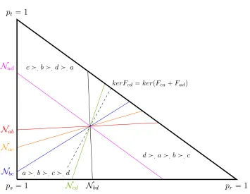
For any subset E of A, the set of p in ∆ satisfying a ą_p b for every b P E is denoted by BapEq, thus a is (strictly) better than every element of E for all

p P BapEq. Similarly, for any subset E of A, the set of p in ∆ for which b is

strictly preferred to a for all b P E is denoted WapEq, so that a is (strictly)

worse than every element ofE for eachpPWpEq. We will make extensive use

of the shorthand Bab for Baptbuq and similarly Wab :“Waptbuq ” Bbptauq “:

Bba. Finally, the set of pP∆ for which a„p b will be called Nab, and the set

Nabc is defined astpP∆ : a„p b„p c„p au.

We make use of the fact that S has n elements to identify ∆ with the n´1

dimensional simplex inRn_, _t_p_P _Rn

` :p1 ` ¨ ¨ ¨ `pn“1u, whereRn_` is the set

of vectors inRn _{for which every element of the vector is strictly positive, and}

s

Rn

` will denote the closure of this set in Rn, that is

s

Rn

`:“ tpP Rn:pi ě0 for all i“1, . . . , nu.9

9

We prefer this notation on the grounds that it is more in line with modern notation used in the mathematical community outside economics. The standard notation in economics beingRn

`` for the strictly positive vectors andR

n

(34)

Where useful, we will consider ∆ as a subset of Rsn´1

` , that is we will identify

each probability distribution in ∆ with a point in the set tp P Rsn´1

` : p1 ` ¨ ¨ ¨ `pn´1 ď1u. In appendix (1.B) of this chapter, we provide some essential

results that justify the relationships between these spaces.

1.2.2 Motivation for the canonical setting

In this thesis we will look at how and when it is possible to use a real-valued

function to characterize and represent the preferences over a set of alternatives

of a decision-maker facing variety of contexts in which the decision problem

may arise. In the canonical decision problems upon which the following

expo-sition predominantly focuses, one way to view the decision problem is in terms

of a decision-maker with the following knowledge:

i. she knows she will face a decision in the presence of uncertainty about

the future state of nature;

ii. she knows, that when the situation arises, she will have sufficient

infor-mation to be able to identify the likelihood of any given state of nature;

iii. given any probability distribution over states, she knows whether or not

she has a strict preference for one course of action, in response to the

uncertainty, over another.

The flood example we have discussed above is an instance of this situation.

We also introduce the next example where there are three states and three

alternatives.

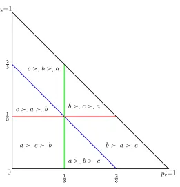
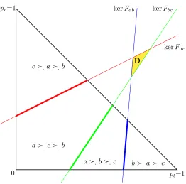
Example 1.3(Getting to and from University). Val lives near her university

(35)

university. Thus A :“ ta, b, cu with a:=“walk”, b:=“bus” and c:=“cycle”.

Suppose that the following conditions hold:

(i) bicycles are not allowed on the bus;

(ii) the bike may be stolen if it is left on campus overnight; and

(iii) the cost of return bus ticket is significantly cheaper than two singles.

These conditions contribute to Val’s strict preference for traveling by the same

means to and from university on any given day. This means that her decision

to buy a bus ticket or ride the bicycle to university in the morning amounts to

a commitment to a single means of travel for the whole day. Of course if she

walks to university, she can catch the bus back, but if she knows that conditions

will be such that in the afternoon she would certainly not want to be walking

home, then she would always buy the ticket, say, in the morning.

As is typical in Autumn, the weather may vary substantially during the day,

and Val knows that it may be raining, sunny or snowing/icey when she returns

that day: soS :“ tr, s, tuwithr:=“raining”,s:=“sunny” andt:=snowing/icy.

Before setting off each morning, the radio weather forecast gives her the chances,

p“ ppsqsPS, of each of the states obtaining.

Fed up with deciding each day, Val decides, once and for all, to devise a

com-plete, contingent plan of what to do. At the time she makes her plan, the set of

contingencies is the set ∆. (Here ∆ is isomorphic to the 2-dimensional, unit

simplex in R3

(36)

Suppose that if she were certain it would be sunny in the evening, Val would

strictly prefer walking to cycling to going by bus, ie. a ą_s cą_s b.10

When it

will rain for sure, her preferences are cą_r bą_r a and when it will snow or be icey for sure, her preferences areb ą_taą_t c.

It seems plausible that Val’s preferences conditional uponp, tpA,ąpq:pP ∆u,

will vary with the probability she face on any given day: the question is how.

Suppose that at the probability p “ p1 3,

1 3,

1

3q, Val’s strict preferences are the

same as they are when statet occurs for sure. Is it then plausible for instance

that, for all probabilities qpλq such that qpλq “λδt` p1´λqp and 0ăλă1,

Val’s strict preferences are unchanged? That is, if we start at a given context

qp0q ” p and increase the probability of state t in such a way that the ratio

of the probabilities of state r and s remain unchanged, does strict preference

remain the same? If so then we conclude that the setconvpδt, pqis a subset of

tpP ∆ :b ą_t aą_tcu ”BbaXBac.

Whilst context preferences of the canonical form presented above are well

suited to modeling the above example, which might be viewed as a game

against nature where nature presumably does not respond to Val’s choices:

they are arguably inadequate for the analysis of strategic game

rock-paper-scissors, where a player is penalized for being predictable or where preferences

may be defined over correlated strategies. We discuss this matter further in

chapter 4.

10

(37)

Remark 1.1. The time-line of the example above has three obvious stages: the

final stage, after both the action has been taken and the uncertainty is resolved;

the penultimate stage, when the agent must act; and the first stage, when the

problem is contemplated and a complete, contingent plan of which action is to

be taken in the penultimate stage is laid out by the decision-maker.

Our focus is on behaviour in the first stage. In the language of Hammond

(1981) we are taking the “ex-ante” approach to choice under uncertainty /

risk. In this thesis no considerations will be given to the optimal time to act.

Similarly, the related question of what constitutes “sufficient information to be

able to identify the likelihood of any given state of nature”, as stipulated in (ii.)

above, is also avoided. That is to say, we model neither the process, nor the

assumptions on behaviour that are involved in the decision-maker converting

information about the uncertainty into beliefs and deciding whether or not to

act.

Of the three basic assumptions on the knowledge held by the decision-maker

(iii.) is the strongest and most questionable; although it is not as strong as

it may at first seem. This is because the decision-maker is free to have

no-strict-preference for one action over another: for every possible probability

distribution over states, and such preferences would not necessarily indicate

indifference.

It is a central tenet of this thesis that even when precise information regarding

the uncertainty is available, choosing between courses of action may still be the

(38)

to understand and weigh-up the differences between the alternatives available

to her. So all other things being equal, a model in which the domain of

pref-erences is minimal and observable to the modeler ought to dominate others.

Not enlarging the domain of preferences comes at the price of requiring that

the agent is able to imagine, or recall from past experience, what her

prefer-ences are in situations different from the present context. That is, we place

greater demands on her ability to imagine variations in the circumstances she

may face in the second stage. Whilst there is no denying that this is the main

drawback of this approach, it is a weaker assumption than to assume

prefer-ences over contexts and alternative-context pairs.

Finally, defining preferences on an observable domain such as actions rather

than the much more abstract concept of outcomes or consequences, that may

or may not be dependent upon states or other factors, brings the model closer

to those that deal with choice functions and observed behaviour. As is the case

in that literature, it may well turn out that the decision-maker behaves as if

she were contemplating all the outcomes and/or consequences of her actions.

If so, this will be an output of the model rather than a starting point.

1.3 Expected utility for context preferences

Given that our canonical example is a model of decision-making under risk or

uncertainty, it is necessary to discuss in more detail the variety of approaches

that already exist. This section provides an exposition of the different models

(39)

really only one candidate for context preferences.

1.3.1 The function-space approach to expected utility

A initial demonstration of why the standard approaches will not work and

why new inter-context conditions are necessary is provided by the following

discussion. We consider a theorem for finite alternative and state spaces by

Adams (1965) and Fishburn (1979). It will show that in our setting, where

a complete contingent plan for each p is the objective, the theorem of

Fish-burn gives a family of additive representations, one for each p. However, as

the condition has nothing to say about how preferences vary with p, it is not

sufficient to ensure linearity inp.

Let As denote the set of outcomes in state s of each of actions in A. The

next theorem defines preferences on ˆn s_“1As.

Example 1.4. In example 1.3 recall that

A:“ twalk, bike, busu ” ta, b, cu, and

S:“ train, sun, snow{iceu ” tr, s, tu.

It is not only arrays of outcomes such as par, as, atq (which may be identified

with the alternative “walk” lie in Ar ˆ As ˆAt) that lie in the domain of

preferences; the idealistic but unfeasible array pcr, as, btq is also there. As a

result even in a simple problem such as this the cardinality of the space Arˆ

AsˆAt is 27, whereas AˆS “9.

(40)

pα1

, . . . , αJ_q_E

Jpβ1. . . βJq if and only if J ą 1, αj, βj P ˆns“1As for j “

1. . . , J, and it is true for eachs thatα1

s, . . . , αJs is a permutation ofβ

1

s, . . . βsJ.

For a fixed, suppressed context we have the following result.

Theorem 1.1 (Scott and Suppes (1958), Fishburn (1979)). The relation ą.

onˆn

s“1As satisfies the following condition: for all J-sequences,tαjuandtβju

in ˆn

s“1As, and all J “2,3, . . .

(F) if pα1

, . . . , αJ_q_E

Jpβ1, . . . , βJq and pβj ą.αjq for j “1, . . . , J´1,

then pαJ _ą .βJq,

if and only if there exist real valued functions u1, . . . , un onA1, . . . , An

respec-tively such that, for all α, β P ˆn s“1As,

p4q αą_.β ô ÿ

sPS

`

uspαsq ´uspβsq

˘

ą0.

One problem with the condition (F) in the above theorem is that it is somewhat

difficult to evaluate without case by case verification. Moreover verification is

by no means an easy task: in example (1.3) where there are three alternatives

and three states, in order to verify the condition, we have to make `272

˘

“351

comparisons.

Another problem with the above representation is that it gives us no

informa-tion about how preferences vary with the context that is the current belief.

Presumably, for context preferencespą_p, pP∆pSqq, the theorem holds for any given p, and the representation is as follows:

p5q αą_p β ô ÿ

s_PS

`

uspαs, pq ´uspβs, pq

˘

(41)

If we seek a representation that has more structure, and thereby resembles a

plan of action we need more conditions on how preferences vary with context.

Chapters 2 and 3 provide two approaches to dealing with this problem.

By contrast, the classical approach to adding more structure has been to

sup-press reference topand focus on state-preferences. In the Anscombe-Aumann

(1963) approach, the first step is to restrict the space of outcomes to be the

same in each state and define lotteries over these outcomes.11

The second step

is to impose that the ordering of the set of outcomes in each state is the same

across states. This state-independence allows us to identify the actual

proba-bility measurep that represents the information context (beliefs) of the agent

at decision time. Thus the Anscombe-Aumann approach says nothing about

how preferences vary with the information context, and hencep. Perhaps it is

best to view this model as capturing behaviour at stage two in the time-line

we describe in remark (1.1) above.

The same may be said of the models of Savage (1954), Scott and Suppes

(1958), and Debreu (1959). They seem to be more appropriate for addressing

the problem of an agent making a decision in the heat of the moment and at a

particular information set. By contrast, the present approach is closer in this

sense to [vNM] where a complete, contingent plan of action is outlined in the

first stage.

11

(42)

1.3.2 EU for context preferences

Let us consider the form of an expected utility (EU) function representing

the preferences of an agent over a set A given the knowledge of a probability

distribution, p, over the state space S.

Definition 1.2 (EU function representation of context preferences).

U :Aˆ∆ is an EU representation of context preferences if both the following

are true:

i) there exists u:AÑRn _{such for all} _p _in _∆ _and _a _in _A_,

Upa, pq “Epupaq:“

ż

S

upa, sqdppsq `or ÿ

s_PS

psuspaq

˘

;

ii) U is said to represent context preferences,tpA,ą_pq:pP∆u, if, for every

pP ∆and a, bPA we have

a ą_p b ô Upa, pq ąUpa, pq.

From the above definition, it is clear that the vector-valued functionu :AÑ

Rn _{characterizes the representation. Indeed, the set} _N

ab is contained in the

hyperplane perpendicular to this vector. As we describe in appendix (1.A),

the elements of this vector-valued function are called state utility functions.

The rationale is simply that if ps “ 0 for all s ‰ t then the decision maker

would face statet with certainty, so that the expected utility Epu“ut which

represents state preferencesą_t. The essence of this EU representation is that preferences atp are represented by the weighted average of the state-utilities,

(43)

s.

1.3.3 Incomparability across states

Suppose context preferences give rise to a representation that is cardinally

measurable but non-comparable across states (CNC across states). In this

case, as the following discussion shows, it is not clear whether probability

plays any role at all. First we define thesupport and null-sets of a probability

measure.

Definition 1.3 (Support of p). For countable S, the support of a probability

measure p, denoted suppppq, is the set of elements of S for which p assigns

positive measure. Thus, suppppq:“ tsPS :psą0u.

Definition 1.4 (Null-sets ofp). The null sets of a probability measure p, are

these for which p assigns zero probability. That is, if T Ă S and ppTq “ 0,

then T is a null set.

Let preferences be represented byU and fix pP∆. LetT be set of states such

thatpt“0. As preferences are CNC, any other functionV :Aˆ∆ÑRthat

is also and EU representation satisfies the property that there existsv :AÑR

such that for each s PS, vs “λsus`κs for some λs ą0 and κs PR. For all

sPT let qs “0. Then for all sPSzT, let 0 ăqs ă1 and letλs :“qs{ps, then

we have

ÿ

s

psuspaq ą

ÿ

s

psuspbq ô

ÿ

s

psλs

`

vspaq ´vspbq

˘ ą0 ôÿ s qs `

vspaq ´vspbq

˘

(44)

so that if the qs sum to 1, the latter is an equivalent representation indexed

by the probability q. In particular this means that for all a and b in A, the

relative interior, ri ∆, of ∆ is a subset of one (and only one) of the sets Bab,

Nab and Wab. This rather extreme property of preferences fact has lead many

authors in the literature to suppress the probability altogether (see Fishburn

(1970) Ch.4 and 5, Debreu (1959)), so that the representation takes the form

ř

sws, with ws :“ psus for each s. Indeed, it seems reasonable to say that

pws, s P Sq characterizes the representation of preferences ąp. This kind of

representation, contrary to what one might think, is in fact overly restrictive

in that it rules out whole classes of preferences without any clear reason.

1.3.4 vNM representation of context preferences

CNC preferences are in contrast to the class of state independent models of

[vNM] and Anscombe and Aumann (1963). Now suppose the context

prefer-ences give rise to a [vNM] type representation on consequprefer-encesY “AˆS. The

resulting utility function is characterized by a single utility functionu:Y ÑR

and for every π and ρ in ∆Y we have

πąρ ô ÿ

xPY

πxupxq ą

ÿ

xPY

ρxupxq. (1.3)

Recall that if v also satisfies the above equivalence then we should have

v “ k `lu for some k P R and l ą 0.That is, preferences are cardinally

measurable and fully comparable (CFC–again see the appendix to this

chap-ter for more on these concepts). As k and l do not vary with s, for given

preferences, the vNM axioms define a much smaller invariance class of

(45)

In seeking to retrieve “response” or context preferences from a vNM

repre-sentation,12

we restrict attention to elements π of ∆Y such thatπ “pˆµ for

somepP∆S and µP ∆A that is elements of ∆Sˆ∆A (where ∆A is the set of

probability distributions on A). Preferences over ∆Y restricted to pˆµ and

pˆν in ∆S ˆ∆A, lead to the representation characterized by u: Y ÑR in

the following way. For each b and c inA:

δb ąp δc ô

ÿ

pa,sqPY

psupa, sq

`

δb´δc

˘

ą0

ô ÿ

sPS

ps

`

upb, sq ´upc, sq˘ą0.

In contrast with CNC preferences, there are now far fewer restrictions on the

sets Bab, Nab and Wab. Of course, each of these sets must be convex, and if

either ofBab and Wab is nonempty, then Nab is thin (empty interior relative to

∆).

Consider the special case where, for all a and b, either a dominates b for

all s P S or the reverse holds for all s P S, then for every a and b, convexity

implies that ∆ is equal to eitherBab orWab. In this case, ∆ lies in a “chamber”

defined as the interior of an intersection of the`n2

˘

open half-spaces defined by

the hyperplanes tIab :a, bPAu.

This in turn implies that we may rotate, by a suitably small amount, the

12

(46)

vectorsupaq ´upbq, keeping ∆ in the corresponding chamber, to obtain a new

functionv :AˆS ÑRthat characterizes some expected utility representation

V and such thatv ‰l u`k for any lą0 and k PR.

Thus a vNM representation, to borrow from the language used in the social

choice literature13

,may imply a good deal more information regarding the

de-cision maker’s preferences than can be observed from context preferences alone.

Even in the case where for every a, b in A, the sets Nab of full dimension

and the hyperplanes Iab are fully identified, the appropriate degree of

com-parability for an EU representation of context preferences will turn out to be

“unit comparability” and the resulting representation is referred to as CUC. It

is characterized by an EU function with the property that the state utilitiesus

in the vector-valued function u:AÑRn_{, are unique up to a common scale}_l_,

but independent origink. That is, if v corresponds to another representation

of the same preferences, then vs “ l us`ks. We derive such a representation

in chapter 2.

More generally, there appear to be no conditions one can meaningfully impose

on preferences that ensure the existence of an expected utility representation of

context preferences. This means that by insisting upon such a representation

we are excluding perfectly reasonable preferences from the analysis without

any real justification. This provides motivation for the third and fourth

chap-ters.

13

(47)

1.4 Synopsis

Chapter 2 presents a model that is closely related to Gilboa and Schmeidler

(2003) (GS03). In this paper, the authors provide a re-interpretation of their

model ofcase-based decision theory and work in the same context space as we

do in this thesis. That is, where states play the role of cases and probabilities

or beliefs play the role of context. We improve upon their model in two

re-spects.

Firstly, we weaken the diversity condition in an important way. Secondly,

we provide an alternative to the “combination” condition of GS03 that gives

rise the linear form of the representation. The resulting conditions are weaker

and we argue more intuitive.In addition, this chapter also sheds light on the

role of expected preference representations (similar to those of Vind (1991))

for context preferences. Expected preference representations are inseparable

across pairs of alternatives, but still linear in probabilities. They can be used

to model intransitive preferences just as well as transitive preferences. As such

it provides way of axiomatizing of the Loomes and Sugden (1982) model of

intransitive regret. This is in the presence of much simpler axioms than

Fish-burn’s skew-symmetric bilinear model.

Chapter 3 proposes a model that gives rise to a utility representation that

is simply order-preserving over alternatives and continuous over contexts. We

identify the most general type of context space for which we can hope to

guarantee a continuous representation. The mathematics of this approach is

(48)

In due course we intent to extend this model to provide a link between decision

theory and the discrete choice models of econometrics on the one hand and

neuroscience on the other.

In the fourth and final chapter we suppose that the decision-maker is

will-ing to extend the domain of preferences to include the space of contexts. That

is, the decision-maker is willing to make statements of the form: “I prefer to

be in context p and choose alternative b than to be in context q and choose

alternativec”. Despite this extension, the domain of preferences is still much

smaller than the [vNM] model of expected utility requires.

As a result, rather than a single mixture space–as defined in Herstein and

Milnor (1953)–we work with a collection of mixture spaces indexed by the

al-ternatives. This leads us to introduce a condition that “bridges” the gaps in

the order between the mixture spaces. The resulting representation resembles

that of [vNM] in that it is both state and context independent, but is

distin-guished by the fact that the uniqueness of the representation depends on the

number of components preferences generate. Methodologically speaking, the

closest models in the literature to the model of this chapter is that of Karni

and Safra (2000) as well as Fishburn’s multilinear utility model.

Our main conclusion is that when preferences vary with context, unless the

decision-maker is willing to extend the domain of preferences to include the

context space, we should only hope for preferences to have a linear utility

representation (as in expected utility) in mathematically interesting but

Context and decision : three approaches to representing preferences

Context and Decision:

Three approaches to representing preferences

Patrick Haralabos Desmond O’Callaghan

Thesis

Doctor of Philosophy

Warwick Mathematics Institute

Contents

Acknowledgments

Declarations

Abstract

Chapter 1

Introduction

1.1

Context and decision: the general case

1.1.1

The role of context

1.1.2

Preferences and utility: the classical approach

1.1.3

Context preferences

1.2

Context and decision under uncertainty

1.2.1

Notation for the canonical setting

1.2.2

Motivation for the canonical setting

1.3

Expected utility for context preferences

1.3.1

The function-space approach to expected utility

1.3.2

EU for context preferences

1.3.3

Incomparability across states

1.3.4

vNM representation of context preferences

1.4

Synopsis