On Analysis and Design of
Algorithms for Robust Estimation
from Relative Measurements
Nelson P.K. Chan
30 March 2016
MSc. Systems & Control
Specialization: Control Theory
Chair: Hybrid Systems (AM)
Graduation Committee:
prof.dr. H.J. Zwart (UT)
dr. P. Frasca (UT)
Abstract
The problem of estimating the states of a group of agents from noisy pairwise difference mea-surements between agents’ states has been studied extensively in the past. Often, the noise is modeled as a Gaussian distribution with constant variance; in other words, the measurements all have the same quality. However, in reality this is not the case and measurements can be of different quality which, for a sensible estimation, needs to be taken into account. In the current work, we assume the noise to be a mixture of Gaussian distributions.
Our contribution is two fold. First, we look at the problem of estimation. Several Maximum-likelihood type estimators are considered, based on the availability of information regarding the noise distributions We show that for networks represented by a tree, the quality of the mea-surements is not of importance for the estimation. Also, the WLSP yields the best performance among the approaches considered. Furthermore, the benefit of the approaches as presented in this report as opposed to the least squares approach is apparent when a graph is more connected. Second, we consider also the problem of adding new edges with possibly unknown quality to the network with the aim to decrease the uncertainty in the estimation. It is observed that the first few edges will more likely add edges which are not close to each other for the cycle graph, or edges which have initially a low value for the degree, that is they have a few neighbors.
Preface
If you take a journey because you love to reach a destination, you may not arrive. But if you love the journey, you can reach any destination. ∼Alexander den Heijer
The work presented in this report is the result of a journey that lasted for approximately9months
as the final hurdle towards reaching the destination (referring to the MSc. degree). In hindsight, it has been quite a pleasant time spent on learning how to do research. Along the course of the journey, I had managed to have some Aha! moments but most of the time I was faced with a brick wall and the time was spent on how to overcome these brick walls.
In the following, I will spend a few paragraphs (which will cumulate to some pages) to extend my sincere gratitude to a number of people (this is rather a long list) whom have helped me throughout this journey and also the MSc. journey in its entirety.
As the report (which my hope is that you would have a look through it after reading these pages) is regarding networks, I will consider the persons I mention hereafter to be nodes (or a cluster of nodes) which are linked to me.
First, I would like to say a huge grazie mille to dr. Paolo Frasca, my supervisor for both the internship and the graduation project. Paolo, I remember our first connection was that of a course instructor - student connection; you being the course instructor for “Hybrid Dynamical Systems” and I the student who took it as part of my curriculum. Until now, I smile when recalling the joke you made in one of the lectures in which you told you were not supposed to talk when you were facing with your back towards the students. Our connection took a turn when I approached you in the summer of2014asking for recommended reading related to a MSc.
topic, which happens to be estimation from relative measurements (The topic of this report). This event had led me to spending a period abroad in Padova, Italy for my internship and also doing the graduation project under your supervision. Looking back, I am grateful to you for enabling these events to occur. To me, it has been a joyful period working under (or with) you. I sometimes ask myself how it is possible that we could have meetings in which we (or I) lost track of time; needless to say, during those fruitful discussions, you have always managed to steer me to the right direction. Furthermore, I need to also thank you for your efforts in my search for a PhD position. Moreover, you have granted me the opportunity to collaborate on a paper with you, which I am also grateful for.
Next, I would like to thank prof.dr. H.J. Zwart and dr.ir. J. Goseling for putting time aside to read my report and to serve as part of the assessment committee. Thank you.
A‘Dankjewel’can also be attributed to Mrs. Marja Langkamp, the secretary of Hybrid Systems, and Mrs. Mirande van der Kooij, from BOZ for taking care of the administration regarding the graduation, especially those long e-mails.
Mrs. Belinda Jaarsma-Knol, also a‘Dankjewel’to you, this time for the administration that was needed for the internship, but in particular for allowing me to pass by your office and just have a talk with you regarding traveling. I will remember one of the encounters in which you told me to smile when my face ‘told’ you I was quite stressed.
Mrs. Lilian Spijker, I cannot forget you. You have been with me since I was, back then, a MSc. student in Applied Mathematics. You have always been listening to me, when I had problems, when I was facing difficulties, but also when I made some progress with the courses. Through your patience and your openness, I have found myself from reluctantly meeting you to actually looking forward to meeting you. You have been a source of encouragement for the past two and a half years and I am in hindsight happy you sent that e-mail to me back in October 2013, which started the link between us.
out to me and for the ‘light’ discussions whenever we do not feel like working (Shh).
Xinwei, xie xiefor always listening and trying your best to answer the math-related questions that I have. Through our discussions, I have learned to appreciate the theorems and it is also thanks to your observation that the moments of a pdf is simply an integral that has led me to solve the problem related to calculating the moments of the two-sided normal tail distribution and as a consequence proposition 2.9 and proposition 2.10 can be shown, one of the Aha! moments!
Connie Wong & Angela Cheung, thank you for setting aside time to talk to me. Connie jie jie, I am indebted to you for the life experiences you have shared with me. In talking to you, I have learned to view a problem from the perspective of others and in doing so understand the motivation for their behavior. Angela, thank you for answering my calls when I felt bored and needed company. Also, thank you making the get-aways to Rotterdam enjoyable.
The following few lines are meant for the Surinamese friends here in Enschede. Ignaas, Cyrano, Annemieke, Jina, Chefiek, Roswita, Eline, Dinah, and all the other members of the Surinamese student community in Enschede, thank you for the support the past years. The year-end gathering, the meet-up in the city center, etc. and for organizing twice a birthday party for me (yup); well what can I say other than thank you.
Now I come to “The Fellowship of the Ring”, the close group of friends consisting of Mohamed, Hengameh, Gisela, Armando, Abhishek, Charalambos, Carlos, Giuseppe and others. Thank you for letting me in be part of the “Fellowship”. We have spent quite some time in the library finishing the courses (Yes, I know you do not want to be remembered about that period!). Also thank you guys for the cinema breaks! Of course I cannot forget the Eqyptian habibi’s Shamel, Adel, and Shamer and the Nigerian friends Bobo, and Victor. Not to mention, William Lee. Thank you all!
A word of thanks also to Femi for providing me shelter for the past couple of months and more for keeping up with me. Also the life experiences shared in the living room. Zan-Bo for free coffee (at least once a day) and for discussions considering graphs.
ICF-Enschede has been a “Home away from Home”. Here, I have found motivation when I was facing difficulties and I also got the opportunity to meet people from different countries. I am also grateful for being given the opportunity to be a member of the choir and also be involved in the student leadership.
I am indebted to AdeKUS, my home university in Suriname for the financial support and in particular, for not giving up on me even though the journey was far from smooth during the first six months in the Netherlands.
Mom and Dad and Sis, thank you for your unconditional love, your support and for the opportunity to let me go after my dreams. Ironically, our physical distance (you in Suriname and I in the Netherlands) has actually drawn us closer to each other.
I would also like to say thank you to all the others with whom I have made a connection in the past two and a half years. There are so many of you but due to space I have to end here. I thank G.P. van der Beek for allowing me to use his template for the coverpage.
The last person I want to thank is God without whom all these people and the experiences I have mentioned above would not have been possible. He has been faithful to me, putting the right people at the right time in my life guiding me according to his desired plan.
I started this part of the report with a quote so I like to end it also with one, this time taken from the bible;
For I know the plans I have for you, declares the Lord, plans to prosper you and not to harm you, plans to give you hope and a future. (Jeremiah 29:11 NIV)
Contents
Abstract i
Preface iii
Contents v
1 Introduction 1
1.1 Motivation . . . 1
1.2 Related Work . . . 1
1.3 Approach . . . 2
1.4 Contribution . . . 2
1.5 Outline . . . 3
I On Algorithms for Robust State Estimation from Noisy Relative Measurements 5 2 Robust State Estimation from Noisy Relative Measurements 7 2.1 Overview . . . 7
2.2 Measurement Model . . . 7
2.3 The Case of Knowing the Quality of the Measurement Noise; WLS Approach . . . . 9
2.3.1 Case: Z¯ is fixed;Z¯ = ¯z. . . 12
2.3.2 Case: Z¯ is random . . . 13
2.3.3 Simplification of the Matrix Product ATWA†ATWQWA ATWA† . . . 14
2.4 The Case of Not Knowing the Quality of the Measurement Noise . . . 16
2.4.1 WLSP Approach; Having Access to the Noise Realization . . . 16
2.4.2 Brute Force Approach; Considering all possibleˆzcombinations in the sample spaceZˆ . . . 25
2.4.3 EM Approach . . . 26
3 Numerical Results 31 3.1 Overview . . . 31
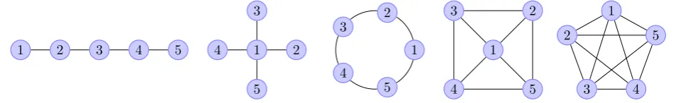
3.2 Graph Configurations Considered . . . 31
3.3 Implementation . . . 33
3.3.1 Comparison of the Exact and the Approximate Approach for MSE of WLSP Estimator . . . 33
3.3.2 Comparison of EM Implementations . . . 34
3.4 Trees . . . 36
3.5 Cycles . . . 36
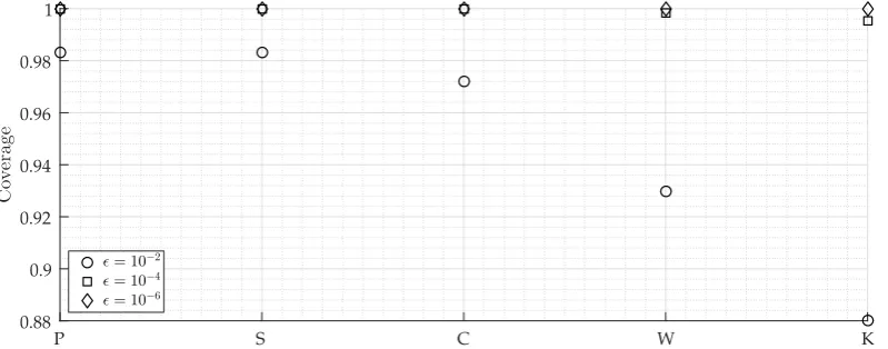
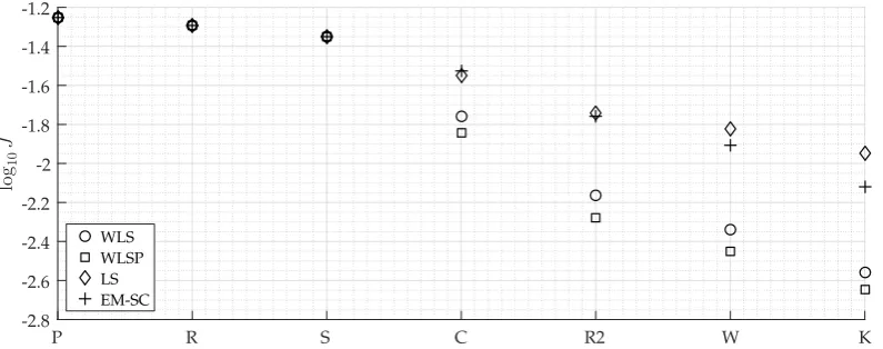
3.6 Five Nodes Graphs . . . 36
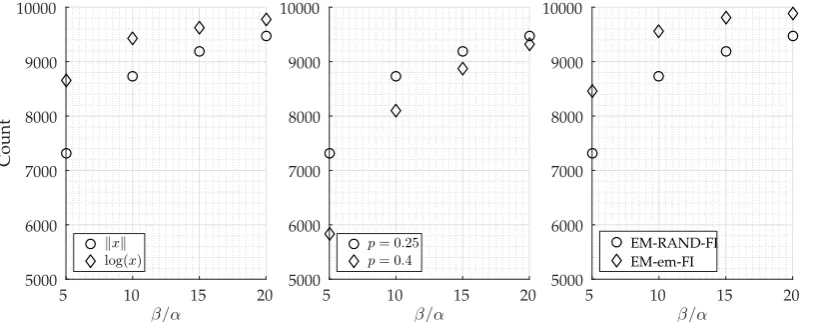
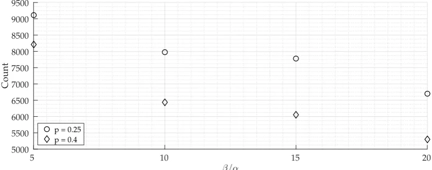
3.7 Parameter Study for a Ten Nodes Graphs . . . 40
4 Conclusion & Outlook 45 4.1 Outlook . . . 45
II On Design of the Network Topology for Improved Estimation 47 5 Optimal Extension of the Graph 49 5.1 Overview . . . 49
5.3 Combinatorial Approach; Adding Edges All at Once . . . 50
5.4 Submodular Approach; Adding Edges One at a Time . . . 51
6 Numerical Results 55 6.1 Overview . . . 55
6.2 Evaluation of the Combinatorial and the Submodular Approaches . . . 55
6.2.1 Ten Nodes Cycle Graph as Base Graph . . . 55
6.2.2 Random Graph as Base Graph . . . 57
6.3 Performance of the Cycle Graph After Edge Addition . . . 58
7 Conclusion & Outlook 61 7.1 Outlook . . . 61
III Appendices 63 A Graph Theory 65 A.1 The Adjacency Matrix . . . 66
A.2 The Degree Matrix . . . 66
A.3 The Graph Laplacian Matrix . . . 66
B The Moore-Penrose Pseudoinverse 69 C Normal Probability Distribution 71 C.1 General Normal Distribution . . . 71
C.2 Two-sided Truncated Normal Distribution . . . 71
C.3 Two-sided Normal Tail Distribution . . . 72
1.
Introduction
1.1 Motivation
Wireless sensor network (WSN) is a relatively new field that has gained world-wide attention in recent years due to advances in technology and the availability of small, inexpensive, and smart sensors which leads to cost effective and easily deployable WSNs [1–3]. In Ref. [1], WSNs is con-sidered as one of the most researched areas in the last decade. This can be justified by a quick online search in which several survey papers are being published addressing the developments within the field and also the challenges that researchers are facing, see for example the references mentioned in Ref. [1]. The building blocks of a WSN are the sensor nodes; tiny devices, which are equipped with one or more sensors, a processor, memory, a power supply, a radio, and possibly also an actuator [2]. These devices are usually spatially distributed and work collectively, hence forming a network. Due to the numerous advantages, such as, lower costs, scalability, reliability, accuracy, flexibility, and ease of deployment, that WSN offers, it is being employed in a wide range of areas. These include among others, fields as military, environmental, health care, industrial, household and in marine applications [1, 2]. As mentioned earlier, sensor nodes are being pro-duced which are small and inexpensive. This unavoidable put resource constraints on the nodes, including a limited amount of energy, short communication range, low bandwidth, and limited processing and storage [2]. Due to the short communication range, each node can communicate only with neighbouring nodes which are within a distance apart from it. As WSN covers spatially a large area, this subset of neighbouring nodes is usually small [4]. Furthermore, a node may usually lack knowledge of certain attributes such as its position in a global reference frame or the global time. These can be attributed as a consequence of the resource constraints. They however, are allowed to obtain a relative value for the quantity of interest between themselves and the neighboring nodes which are as mentioned within a certain distance. Hence, it is desired to obtain global estimates using the set of relative measurements.
1.2 Related Work
A follow-up problem related to the estimation problem regards improving the estimation by means of reducing the uncertainty in the estimation. This may be done by optimally choosing a small set of edges to add to the existing graph. The addition of edges to a base graph with the aim of maximizing the algebraic connectivity of the laplacian has been studied previously in [7, 14]. In Ref. [14], heuristic approaches are considered for the edge addition problem applied to an unweighted graph. A greedy approach is described and compared with the convex relaxation approach. Osting et al. [7] has used this approach and applied it to ranking problems in movie rating and sport scheduling. Herein, the graph considered is weighted.
In the optimal design community, maximizing the algebraic connectivity is considered as the E-optimal condition. Other criteria that may be considered are the A-E-optimal problem in which the negative sum of the inverse of the eigenvalues are considered, i.e.,−∑iN=2λ−i 1 and the D-optimal which is the product of the eigenvalues, ∏N
i=2λi. Note, the sum is taken starting fromi= 2, as
we are aware that the first eigenvalue of the laplacian equals zero and the graph considered is assumed to be connected. The A- and D-optimal criteria are less studied while having interesting interpretation. The D-optimal criterion can be interpreted as the number of spanning trees in a graph while the A-optimal criterion is proportional to the total effective resistance of an electric network in which the edge weights are considered to be the resistance between the vertices [7, 15].
In a recent paper [16] by Summers et al., the addition of edges is considered to optimize the network coherence, which is proportional to the A-optimality criterion. A greedy approach is also applied here as a heuristic for adding edges.
1.3 Approach
In the current study, we relax the assumption of homoscedasticity for the noise and assume it to be a binary mixture of Gaussian distributions; as a consequence we can make a distinction between measurements that are considered to be accurate or ‘good’ in quality and measurements that are ’bad’ in quality. For the estimation, these measurements are then weighted differently, putting more emphasis on the ‘good’ measurements in order to still obtain a sensible estimate. Depending on the availability of information regarding the noise distributions, several estimators based on the Maximum Likelihood Principle are derived and its performance are analysed. Apart from the estimation problem, we also look at how to optimally add new edges to the available edge set with the aim to reduce the uncertainty in the state estimates. A comparison is made between the combinatorial approach in which a set of edges is added all at once and the sub-modular approach in which the edges are added one at a time. In this problem we include also cases for adding nodes with unknown quality.
1.4 Contribution
1.5 Outline
Part I
On Algorithms for Robust State
Estimation from Noisy Relative
2.
Robust State Estimation from Noisy Relative
Measurements
2.1 Overview
In this part of the report, our attention will be drawn to the state estimation problem.
In the current chapter, we start by defining the measurement model used in the current work, see section 2.2. The novelty herein consists the noise which is modeled as a Gaussian mixture instead of being a constant variance for each measurement. Hereafter, the following estimators, based on the Maximum Likelihood Principle, are derived depending on the availability of information regarding the noise distribution.
In the Weighted Least Squares (WLS) approach, presented in section 2.3, we assume the quality of the measurements to be known, and hence direct estimation can be immediately carried out. Performance analysis are also presented for this estimator.
Next, we consider the WLSP approach, given in section 2.4.1. In the WLSP approach, with the P stands for “Plus”, we assume to not have the quality of the measurements but are given the original state vector ¯xand when this information is combined with the available measurements b, the actual noise realization vectorηcan be obtained. We derive a classification rule based on the Maximum A Posteriori (MAP) estimation. In particular, a threshold value is obtained which decides whether the noise realization is ‘good’ or ‘bad’. After the classification step, we then proceed with estimation using WLS approach. Performance analysis regarding the estimator are also presented.
In section 2.4.2 and 2.4.3, we assume to be given only the noise distribution parameters in addition to the set of measurements and the graph topology. The task is then to first classify the measurements and afterwards perform estimation based on the measurements. Herein, two approaches are considered; that of a naive brute force approach in which for all the possible combinations regarding the quality of the measurements, the WLS estimate is obtained. In the second step, we then choose the WLS estimate ˆx which yields the highest value for the log likelihood function. Hence, in the current approach we have first performed estimation, with classification following after it.
The second approach we consider is based on the Expectation Maximization algorithm. Herein, hidden random variables are introduced in order to complete the measurement data and we alternate between the expectation step, in which a soft classification,i.e.,zˆ ∈[0, 1]with0referring
to ‘good’ and1to ‘bad’ measurement, is done and a maximization step, which again boils down to
carrying out the WLS approach. In particular, the WLSP approach can be regarded as one iteration of the EM approach in which here hard classification is performed, i.e., zˆ∈ {0, 1}.
2.2 Measurement Model
As mentioned already in the Introduction, we are interested in the problem of estimating the state vector from noisy relative measurements (also known as pairwise differences [17]). Problems of this type include localization [11], time synchronization [4, 17], and statistical ranking [7].
The measurement model is described as follows: we consider a network of Nagents. Each of the agents in the network possesses a quantityx¯i, which is not known to the agents themselves.
In the current work, we assume the quantity to be a scalar value, i.e., x¯i ∈ R. The scalar value
may for example be, the position in localization problems, the clock offset in time-synchronization problems, or the popularity in the ranking problem. The agents are allowed to take relative noisy measurements with their neighbors, a small subset of the network. The goal is to use the set of noisy relative measurements to construct an estimate of the original state vector x¯ ∈ RN.
to each agent’s value will not change the pairwise difference; (x¯i+c)− x¯j+c
= x¯i−x¯j
. Hence the problem is sometimes referred to as finding an estimate of the pairwise diffferences from noisy measurements [17].
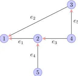
Using terminology from graph theory, the above description can be represented graphically. The agents are regarded as vertices of a graph and the relative measurements as the edges con-necting the vertices; see fig. 2.1 for an example graph consisting of 5 vertices and 5 edges con-necting the vertices in a pairwise manner.
1 2
3
4
5
e1 e2
e3
e4
[image:15.595.222.351.165.290.2]e5
Figure 2.1: An example graph G with vertex set V(G) = {1, 2, 3, 4, 5} and edge set E(G) =
{e1= (2, 1),e2= (3, 1),e3 = (4, 2),e4 = (5, 2),e5 = (4, 3)}.
The set of relative measurements can be encoded using the edge-incidence matrix A ∈ {0,±1}M×N with entries defined as
Aei =
+1 ife = (j,i)
−1 ife = (i,j)
0 otherwise
for e∈ E(G). (2.1)
Note that each row of the Amatrix corresponds to one measurement and we assume to have M measurements. Also, in the above definition, we assume a pair(j,i)to be an element of the edge
setE(G)if and only ifi<j; in fig. 2.1, this is graphically represented by the arrows in which the
orientation is always towards the smallest labelled number of each pair. The A matrix for the graph in fig. 2.1 is
A=
1 −1 0 0 0 1 0 −1 0 0 0 1 0 −1 0 0 1 0 0 −1 0 0 1 −1 0
.
By letting b∈RM to denote the set of measurements, we have
b= A¯x+η, (2.2)
with A¯xthe uncorrupted relative difference between pairs of vertices within the network andη the vector of Gaussian additive noise corrupting the relative difference. We assume the noise to have the following spefications: each noise term have mean zero, i.e.,E[ηe] =0and the variance
equals E
η2e = σe2 ∀e ∈ E(G), with σe2 = (1−z¯e)α2+z¯eβ2, 0 < α < β andz¯e ∼ Ber(p), i.e., z¯e is
Bernoulli distributed and the probability thatz¯e=1, which means N 0,β2 is chosen and hence the measurement is considered ‘bad’, is p. Furthermore, we assume each noise term ηe to be
2.3 The Case of Knowing the Quality of the Measurement Noise;
WLS Approach
In the current case, besides the information regarding the graph topology given by A, the set of measurementsband the noise distribution parameters, we assume to also know the value of z¯e
for each measurement, in other words the quality of each measurement. We have
¯
ze=
(
1 ifηe∈ N 0,β2
0 ifηe∈ N 0,α2
∀e∈ E(G). (2.3)
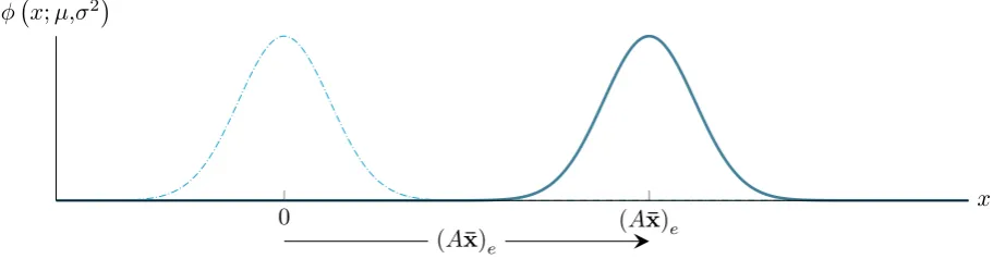
By knowing this additional information, we know P(ηe) ∀e ∈ E(G) exactly and because be = (A¯x)e+ηe, alsoP
be
(A¯x)e
by shifting the distribution ofP(ηe)by the value(Ax¯)e, see fig. 2.2.
(A¯x)e
0 (Ax¯)e x
[image:16.595.79.535.253.372.2]φ x;µ,σ2
Figure 2.2: The equivalence between P(ηe)andP
be
(A¯x)e
.
By the iid (independent and identically distributed) assumption, we have for the joint proba-bility functionPb
¯x
Pb ¯x
=
∏
e∈E Pbe
(A¯x)e
, (2.4)
with
Pbe
(A¯x)e
= p 1
2πσe2
exp − be− x¯i−x¯j 2
2σe2
!
. (2.5)
Subscripteis the pair(j,i)andσe2= (1−z¯e)α2+z¯eβ2. The maximum likelihood estimation (MLE) approach is used in order to obtain an estimate of ¯x when the measurementsbare given. This is based on the following principle:
Definition 2.1 (Maximum Likelihood Principle [18]). Given a dataset, choose the parameter(s) of in-terest in such a way that the data are most likely.
In our case, the data are the measurement vector band the parameter of interest the state vector ¯x. The MLE approach is the most popular technique for deriving estimators [19] and has among others the invariance property, in which if θˆ is the maximum likelihood estimate of a
parameterθ, thenτ θˆis the MLE forτ(θ). Other useful properties of the MLE are the asymptotic unbiasedness and the asymptotic minimum variance property.
The likelihood function is defined as
Lx b
= Lx1, x2, . . . , xN
be∀e∈ E
=Pb x
and according to definition 2.1, we seek to find the parameter valuesx1,x2, . . . ,xN that most likely
have produced the observationsbe∀e ∈ E(G)(Note: the bar abovexis removed to indicate that
xis now the variable.). This is formulated in the following optimization problem:
ˆ
x=arg max
x∈RN
Lx b
. (2.7)
In the following we will work with the log likelihood functionlogLx b
by taking the natural logarithm of the likelihood function Lx
b
. This because in order to solve the maximization problem, we need to differentiate the function and it is easier to work with the log likelihood function as then a product of terms is changed into a sum of the logaritms, Ref. [18]. Also, because the log likelihood function is strictly increasing, the extreme points of Lx
b
and logLx b
coincide [18, 19]. Hence, we obtain
logLx b
=logPb x
=log
∏
e∈E(G) Pbe
(Ax)e
=
∑
e∈E(G)
logPbe
(Ax)e
. (2.8)
The second equality is due to the iid assumption, eq. (2.4) and the third equality by usinglog∏ai = ∑logai.
Proposition 2.1 (WLS Estimator). Let A ∈ {0,±1}M×N be the edge-incidence matrix describing the
graph topology according to eq. (2.1), b ∈ RM the vector of measurements, ¯z ∈ {0, 1}M the vector
indicating the quality of the measurements andαandβthe noise parameters with0 < α < β, then the solution to eq.(2.7)is given by
ˆx=ATW¯zA
†ATW
¯zb, (2.9)
withW¯z =diag (1−z¯e)α−2+z¯eβ−2.
Proof. In order to solve eq. (2.7), we need to take the derivative of eq. (2.8) with respect to the variables xk, k=1, 2, . . . ,Nand set the system of equations equal to zero, i.e.,
∂
∂xk logL
x b
=0, fork =1, 2, . . . , N. (2.10)
As there are N parameters, we have N equations and using the sum rule in differentation, each equation will have M terms corresponding to the number of measurements. For illustration purposes, the derivation for one such term is given below,
logPbe
(Ax)e
=log p 1
2πσe2
exp − be− xi−xj 2
2σe2
!!
.
Taking the derivative with respect to xk yields
∂ ∂xk
logPbe
(Ax)e
= ∂
∂xk
log p 1
2πσe2
exp − be− xi−xj 2
2σe2
!!
= ∂
∂xk
logp 1
2πσe2
+ ∂
∂xk
− be− xi−xj 2
2σe2
!
=− be− xi−xj σe2
∂ be− xi−xj
∂xk
,
with
∂ be− xi−xj
∂xk =
0 if edgee is not connected to vertexk
−1 if edgee is connected to vertexkandk is the “to” vertex
This corresponds to the−Aek entry in the edge-incidence matrix, hence
∂ ∂xk
logP(be|(Ax)e) =
Aek be− xi−xj
σe2 . (2.12)
As mentioned earlier, there are M terms in each of the N equations and each of the M terms will have the same structure as eq. (2.12). Writing the system of equations in matrix form, we eventually obtain
ATW¯z(b−Ax) =0⇔ ATW¯zAx= ATW¯zb⇔ ˆx=
ATW¯zA
†ATW ¯zb.
with W in the above being a diagonal matrix having entries we = (1−z¯e)α−2+z¯eβ−2. The subscript ¯zexplicitly states the dependence ofW on the indicator vector ¯z.
()†in the above denotes the Moore-Penrose pseudoinverse. We take the Moore-Penrose
pseu-doinverse for the product ATW¯zA
is not invertible. Taking a closer look, we can observed that this product is the laplacian of the weighted graph and as the laplacian always has an eigenvalue of zero, it is not invertible, see section A.3 for more information related to the laplacian matrix. ˆxobtained above is the minimum 2-norm solution [20].The estimate ˆxobtained in proposition 2.1 can also be obtained using the weighted least squares (WLS) approach in which we minimize the weighted 2-norm of the difference (b−Ax), i.e.,
ˆx=arg min
x∈RN
1
2kb−Axk
2
W¯z. (2.13)
The derivation can be found in Ref. [21]. In the unweighted case, it is known that minimization of the sum of square errors kb−Axk2is equivalent to maximization of the log-likelihood function
when the observations are independent of each other and the noise is gaussian [22]; the current result can thus be seen as the weighted analogue to that. As already mentioned earlier, we can estimate ¯xup to an additive constant, hence
ˆxW LS = ˆx+c1, (2.14)
with the constantcstill undetermined.
In the following, we evaluate the WLS estimator as we are interested in the properties of the estimator. First, we give some definations of properties that are useful for evaluating estimators. We start with the bias of an estimator:
Definition 2.2 (Bias of an estimator [19]). The bias of a point estimator θˆ of a parameter θ is the
difference between the expected value ofθˆandθ; that is, Bias
θθˆ=Eθ
ˆ
θ−θ. An estimator whose bias is identically equal to0is called unbiased and satisfiesEθ
ˆ
θ=θfor allθ.
We continue with a definition for the mean squared error of an estimator:
Definition 2.3 (Mean Squared Error [19]). The mean squared error (MSE) of an estimator θˆ of a
pa-rameterθ is the functionθdefined byEθ
ˆ
θ−θ2.
The MSE measures the average squared difference between the estimatorθˆand the parameter
θ and can be rewritten as the following
Eθ
ˆ
θ−θ2=Eθ
ˆ
θ−Eθ
ˆ
θ+Eθ
ˆ
θ−θ2
=Eθ ˆ
θ−Eθ
ˆ
θ2+2Eθ
ˆ
θ−Eθ
ˆ
θ Eθ
ˆ
θ−θ
| {z }
0
+Eθ Eθ
ˆ
θ−θ2
=Varθθˆ+ Eθ
ˆ
θ−θ2
=Varθθˆ+ Biasθθˆ
2
The MSE can thus be split in two components, Varθθˆ measuring the variability of the estimator
(precision) and Biasθθˆ2
measuring its bias (accuracy). If the estimator is unbiased, then the MSE equals the variance of the estimator, i.e.,
Eθ
ˆ
θ−θ2=Varθθˆ.
Note that for determining whether the estimator is biased or unbiased, we need to calculate the mean of the estimates which is the first moment of a distribution and the variance the second centralized moment of a distribution.
We consider two cases for the evaluation, first is the case in which we hold the random variableZ¯ fixed, i.e.,Z¯ = ¯zwith ¯z∈ {0, 1}M; second, we consider the case in whichZ¯ is random.
This is seen as a generalization of the former case.
2.3.1 Case: Z¯ is fixed; Z¯
=
¯zThe following proposition sums up the main result of this subsection:
Proposition 2.2 (Moments of the WLS estimator conditioned on Z¯). Let the WLS estimate of ¯xbe given by eq. (2.14)with ˆxobtained from proposition 2.1 and assume Z¯ = ¯zto be fixed. If the additive constant is chosen to be the centroid of the nodes, i.e.,c= mean(¯x), and expectation is taken on the
noise term, given by the random variableH, we can obtain the following:
EH
h ˆxW LS
Z¯ = ¯z
i
= ¯x, (2.15)
and
EH
h
(ˆxW LS−¯x)(ˆxW LS−¯x)T
Z¯ = ¯z
i
=ATW¯zA
†, (2.16)
i.e., the WLS estimator is unbiased and its covariance matrix is given by the laplacian of the weighted graph.
Proof. First, we will prove eq. (2.15).
EH
h ˆxW LS
Z¯ = ¯z
i
=EHhˆx+c1 Z¯ = ¯z
i
=EHhATW¯zA
†ATW
¯zb+c1
· · ·
i
=EHhATW¯zA
†ATW ¯zA¯x
· · ·
i
+EHhATW¯zA
†ATW ¯zη¯z
· · ·
i
+Ehc1 · · ·
i
= ATW¯zA
†ATW ¯zA
| {z }
IN−N111T
¯x+ATW¯zA
†ATW ¯zEH
h η¯z
Z¯ = ¯z
i | {z }
0
+c1
=
IN−
1
N11
T
¯x+c1.
With the choice ofc= N11T¯x=N1 ∑iN=1x¯i
, we obtain eq. (2.15). Plugging this result in eq. (2.14) yields
ˆxW LS = ¯x+
ATW¯zA
†ATW
We proceed by showing eq. (2.16).
EH
h
(ˆxW LS−¯x)(ˆxW LS−¯x)T
Z¯ = ¯z
i
=EHhATW¯zA
†ATW
¯zη¯zηT¯zW¯zA
ATW¯zA
†T · · ·
i
= ATW¯zA
†ATW ¯zEH
h η¯zηT¯z
· · ·
i W¯zA
ATW¯zA
†T
= ATW¯zA
†ATW ¯zQ¯z
| {z }
IN
W¯zA
ATW¯zA
†
= ATW¯zA
†ATW ¯zA
ATW¯zA
†
= ATW¯zA
†.
(2.18)
In the previous derivation, the third equality is obtained using property 2 of the Moore-Penrose pseudoinverse in appendix B and noting that the matrix product ATW¯zA
is the laplacian of the weighted graph, we know it is symmetric, i.e., ATW
¯zA
= ATW ¯zA
T
. The last equality is obtained using the second Penrose equation in theorem B.1.
2.3.2 Case: Z¯ is random
As mentioned already this is the generatization of results obtained from the previous subsection. Before we state the proposition we give the following theorem which will be used.
Theorem 2.1([19]). IfXandYare any two random variables, then
E[X] =EhEhX Y
ii
. (2.19)
Proposition 2.3 (Moments of the WLS estimator). Let the WLS estimate of ¯xbe given by eq.(2.14) with ˆxobtained from proposition 2.1 and assumeZ¯ to be random. If the additive constant is chosen to be the centroid of the nodes, i.e.,c=mean(¯x), and expectation is taken on the noise term, given by the
random variableH, and onZ, then we can obtain the following:¯
EZ¯,H[ˆxW LS] = ¯x, (2.20)
and
EZ¯,H
h
(ˆxW LS−¯x)(ˆxW LS−¯x)T
i
=
∑
z
(1−p)#αp#βATW zA
†.
(2.21)
with#αbeing the number of zeros inzand#βthe number of ones and pthe probability of getting a one.
Proof. Again, we will first prove eq. (2.20). Using theorem 2.1 and the definition of expectation, the following can be obtained
EZ¯,H[ˆxW LS] =
∑
zP(Z¯ =z)EHhˆxW LS
Z¯ =z
i
. (2.22)
In words: for eachZ¯ =z, I can obtain a value for EHhˆxW LS Z¯ =z
i
;EZ,H¯ [ˆxW LS]is seen as taking
the weighted sum ofEH
h ˆxW LS
Z¯ =z
i
with weights given byP(Z¯ =z).
In the above equation, three pieces of information is needed: • ∑z;
• P(Z¯ =z);
P(Z¯ =z) =P M \
i=1
¯
Zi =zi
!
= M
∏
i=1P(Z¯i =zi) = (1−p)#αp#β with#α+#β= M. (2.23)
The second equality is obtained due to the iid assumption and the third equality by the following observation; We know thatzi ∈ {0, 1}with0referring to a ‘good’ measurement
and 1 to a ‘bad’ measurement. The probability of obtaining a ‘bad’ measurement is p.
Grouping the zeros and ones in the vectorz leads to the third equality. • EH
h ˆxW LS
Z¯ =z
i
; may be obtained using proposition 2.2. Putting the pieces together yields
EZ¯,H[ˆxW LS] =
∑
zP(Z¯ =z)EHhˆxW LS
Z¯ =z
i
=
∑
z
(1−p)#αp#β¯x= ¯x.
The last equality is obtained because the sum ∑z(1−p)#αp#β = 1 as we sum over the sample
space of Z¯. From the above we can conclude that the WLS estimator is in its general form unbiased. With the same reasoning, we can obtain eq. (2.21).
2.3.3 Simplification of the Matrix Product ATWA†
ATWQWA ATWA†
In the following, we are interested in obtaining a simpler form for the matrix product ATWA†
ATWQWA ATWA†
by using existing results available for the Moore-Penrose pseu-doinverse in appendix B. The case for whichW =Q−1is already considered in eq. (2.18). There we have found that the simplified form is then ATWA†
. We now consider the case whenW 6=Q−1. This will be useful for the subsequent sections, in particular for the WLSP estimator, 2.4.1.
We first consider rewriting the product ATWA†, by introducing A˜ = ATW1/2.
Proposition 2.4. Let A∈ Rm×nbe a rectangular matrix,W ∈ Rm×ma diagonal matrix and consider
the matrix productA˜ = ATW1/2 ∈Rn×m. Then we have
ATWA† = A˜†TA˜†. (2.24)
Proof.
ATWA†= ATW1/2W1/2A†= A˜A˜T†= A˜T†A˜†= A˜†TA˜†. (2.25)
The third equality is obtained using special case2for the matrix product of theorem B.2.
Now we can state the main result.
Theorem 2.2. Let A ∈ Rm×n be a rectangular matrix, W,Q ∈ Rm×m be diagonal matrices with
W 6= Q−1and consider the the matrix productA˜ = ATW1/2 ∈Rn×m, then we have
ATWA†ATWQWAATWA† = A˜†TW1/2QW1/2 | {z }
WQ=QW
˜
A†.
Proof. Using proposition 2.4, we obtain
ATWA†ATWQWAATWA† = A˜†TA˜†AW˜ 1/2QW1/2A˜TA˜†TA˜†
=A˜†TA˜†A˜W1/2QW1/2A˜†TA˜†A˜T.
(2.26)
The second equality is due to the transpose property (AB)T = BTAT. We consider the product
˜
A†TA˜†A.˜
˜
The second equality is a consequence of applying property4of theorem B.1; the third is obtained
using the transpose property and the fourth equality due to property 2 of again theorem B.1.
Plugging the result in eq. (2.26) yields the desired result. We also note that diagonal matrices commute, i.e., AB=BA, hence the productWQ =QW.
If in addition, matrix A is full row rank, then further simplification can be obtained. This because we can apply special case of theorem B.2 toA˜ due to the observation that ifAif full row
rank, then AT is full column rank. We obtain
˜
A†= ATW1/2† =W1/2†AT† =W−1/2AT†. (2.27)
with the third equality as a consequence of applying property3for Moore-Penrose pseudoinverse
matrices. Application to proposition 2.4 and theorem 2.2, we have
Proposition 2.5. Assume the conditions in proposition 2.4 holds and in addition, we have thatAis full row rank, i.e., rank(A) =m, then
ATWA†= A†W−1A†T. (2.28)
Proof. By plugging the result of eq. (2.27) in proposition 2.4, we have
˜
A†TA˜† =W−1/2AT†TW−1/2AT† = A†W−1A†T.
Theorem 2.3. Assume the conditions in theorem 2.2 holds and in addition, we have that Ais full row rank, i.e., rank(A) =m, then
ATWA†ATWQWAATWA† =ATQ−1A†. (2.29)
Proof. By plugging the result of eq. (2.27) in theorem 2.2, we have
˜
A†TW1/2QW1/2A˜† = A†W−1/2W1/2QW1/2W−1/2A†T = A†QA†T = ATQ−1A†. (2.30)
An alternative way to show the above is to start from proposition 2.5 and then using the property that Ais full row rank and henceAT is full column rank, see property6and7for Moore-Penrose
pseudoinverse matrices.
We end this section by providing the WLS algorithm, given in algorithm 1.
Algorithm 1WLS Approach
Require: Data: (A,b,¯z,p,α,β)
1: Computation of weights:
2: for alle∈ E(G)do
we= 1
−z¯e
α2 +
¯
ze
β2 ∀e∈ E(G)
3: end for
4: Estimation step:
ˆx=ATW¯zA
†ATW
¯zb, withW¯z=diag(w) 5: Additive constant:
2.4 The Case of Not Knowing the Quality of the Measurement
Noise
In section 2.3, we consider the case in which we know the quality of the measurement noise; however, in reality this information is a priori not known; hence an estimation of the measure-ment quality, given by ¯z, needs to be found (also known as the classification step) preceding the estimation of the state vector. Three approaches are presented in which classification and esti-mation are being performed. But first, the log likelihood function will be derived for the current case of unknown measurement quality.
With the quality for each measurement unknown, the probability distribution of the noise term ηe is now a mixture of Gaussian distributions, obtain using the total probability law:
P(ηe)UK =P
ηe
N 0,β
2
P N 0,β2+P
ηe
N 0,α
2
P N 0,α2
=p 1
2πβ2
exp
−(ηe)
2
2β2
·p+ √ 1
2πα2
exp
−(ηe)
2
2α2
·(1−p),
(2.31)
with ∑σ2
e∈{α2,β2}P N 0,σ
2
e
= 1. The subscript UK indicates ‘Unknown’. By shifting the
proba-bility distribution function by (A¯x)ethe conditional probability ofP
be
(A¯x)e
UK is found to be
Pbe
(A¯x)e
UK = p p
2πβ2
exp − be− x¯i−x¯j 2
2β2
!
+ √1−p
2πα2
exp − be− x¯i−x¯j 2
2α2
!
. (2.32)
We again use the MLE approach to obtain an estimate of the state vector given the available measurements. In the current case, the likelihood function is
Lx b
UK = L
x1, x2, . . . , xN
be∀e∈ E
=Pb x
UK. (2.33)
In order to estimate ¯x, we need to maximize the following:
ˆ
x=arg max
x∈RN
Lx b
UK (2.34)
By taking the natural logarithm, we have
logLx b
UK=logP b x
UK=log
∏
e∈E Pbe
(Ax)e
UK =
∑
e∈E
logPbe
(Ax)e
UK. (2.35)
As pointed out in Ref. [23], maximization of the above equation in a direct manner is not an easy task and no closed form exist for the optimal ˆx. Hence, we look for alternatives to solve this maximization problem. In the approaches presented, a 2-step approach is taken; first, the measurements are classified, after which the state vector is then estimated.
2.4.1 WLSP Approach; Having Access to the Noise Realization
In the WLS approach, we assume to know the quality of each measurement ahead of time and hence the noise distribution. In the current approach, we have the inverse and assume to know the noise realization for each measurement. Our goal is then to obtain the noise distribution that most likely have produced the realization and with this information obtain an estimate of the state vector.
stands for ‘Plus’. We will elaborate on the classification step as the estimation step is already considered in section 2.3.
In order to obtain the noise realization, we assume to have ‘temporary’ access to the state vector ¯x. The noise realizationηcan then be obtained using eq. (2.2). We then specifically ask the question: which noise distribution (assuming that we then know the number of distributions that are present, the family of distributions, and the parameters of the distributions) has most likely produced the noise term we observe. This again is an instance of the use of definition 2.1. The question can be formulated as the following optimization problem:
ˆ
σe2= arg max
σe2∈{α2,β2}
PN 0,σe2
be,(A¯x)e
, (2.36)
withPN 0,σe2
be,(A¯x)e
being the posterior distribution of obtainingσe2.
Proposition 2.6 (WLSP Classification with p < 1+1
γ and γ =
α
β). Let A ∈ {0,±1}
M×N be the
edge-incidence matrix describing the graph topology according to eq.(2.1),b∈RMthe vector of
mea-surements, ¯x∈RNthe state vector, and
α,β, andpthe noise parameters with0<α<βandp< 1+1γ withγ= αβ, then we have
ˆ
ze=
1 if ηe > δ
0 otherwise.
∀e ∈ E(G). (2.37)
withηebeing the noise realization andδthe decision boundary given by
δ =
s
2
1
α2 −
1
β2
−1log
1−p p
β
α
. (2.38)
Proof. We start the proof by rewriting eq. (2.36) for we are dealing with only two alternatives for σe2: The following inequality can be obtained:
PN 0,β2
be,(A¯x)e
>PN 0,α2
be,(A¯x)e
,
known in the statistics literature as the Bayes classifier. This classifier produces the lowest pos-sible test error rate, called the Bayes error rate and serves a a standard against which other methods are compared to [24]. Using the Bayes’ theorem, stated as follows
PD E,F
=
PE D,F
PD
F PE
F
, (2.39)
we rewrite the above inequality. In the current case, we have D=N 0,β2or N 0,α2, E=be, F = (A¯x)e.
The derivation is only done for N 0,β2 as the same procedure applies for when D= N 0,α2. Substituting yields
PN 0,β2
be,(A¯x)e
=
Pbe
N 0,β
2
,(A¯x)ePN 0,β2 (A¯x)e
Pbe
(A¯x)e
=
p p
2πβ2
exp − be− x¯i−x¯j 2
2β2
!
p p
2πβ2
exp − be− x¯i−x¯j 2
2β2
!
+ √1−p
2πα2
exp − be− x¯i−x¯j 2
2α2
!.
Note: PN 0,β2 (A¯x)e
= P N 0,β2. As the denominator is the same in the inequality, we only pay attention to the numerator:
PN 0,β2
be,(A¯x)e
>PN 0,α2
be,(A¯x)e
⇔
p p
2πβ2
exp − be− x¯i−x¯j 2
2β2
!
> √1−p
2πα2
exp − be− x¯i−x¯j 2
2α2
! ⇔
exp be− x¯i−x¯j
2 2 − 1 β2 + 1 α2 !
> √1−p
2πα2 p
2πβ2
p ⇔
be− x¯i−x¯j
2
2
− 1
β2 +
1
α2 !
>log
1−p p β α ⇔
be− x¯i−x¯j | {z }
ηe > s 2 1
α2 −
1
β2
−1log
1−p p
β
α
| {z }
δ
.
The fourth inequality is obtained by taking the natural logarithm of both sides. Using the as-sumption that0 <α< β, we have α12 > β12 and hence no sign change occurs when we multiply
both sides with 1
α2 −
1
β2
−1. The condition p < 1
1+γ with γ = α
β is needed in order for the log
term to be greater than0. This can be easily verified. Hence, the proof is given.
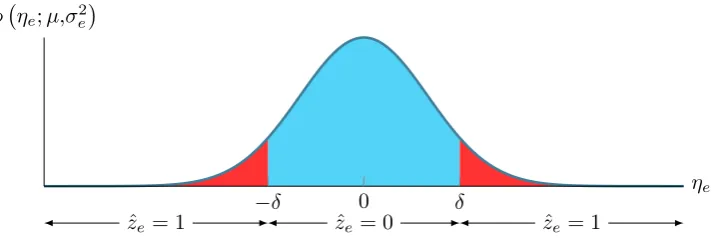
In fig. 2.3, the normal curve is divided into two regions, with the region indicated in blue, the region in which the noise term ηe is classified as to be from N 0,α2 and when ηe is in the red
region, then it is assumed to be sampled from N 0,β2.
ˆ
ze = 1 zˆe = 0 zˆe = 1
−δ 0 δ
ηe φ ηe;µ,σ2e
[image:25.595.113.475.417.536.2]
Figure 2.3: Plot of a normal curve and regions showing classification depending on the realization ηe
In case the condition p< 1+1
γ is not met, we have the following: Proposition 2.7 (WLSP Classification with p ≥ 1
1+γ and γ = α
β). Let A ∈ {0,±1}
M×N be the
edge-incidence matrix describing the graph topology according to eq.(2.1),b∈RMthe vector of
mea-surements, ¯x∈RNthe state vector, and
α,β, andpthe noise parameters with0<α<βandp≥ 1+1γ withγ= αβ, then we have, regardless ofηe,
ˆ
ze=1 ∀e∈ E(G). (2.41)
Proof. Withp ≥ 1
1+γ, we have that the log term in eq. (2.38) is negative and as such,δis a complex
value with real part zero, i.e.,
δ =0+i
s −2
1
α2 −
1
β2
−1log
1−p p
β
α
Hence ηe
> δ is always true as ηe
> Re(δ) = 0. The noise term is thus regarded as to be sampled from the distributionN 0,β2
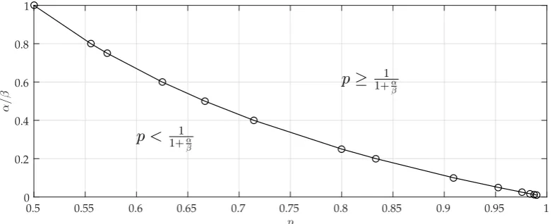
In fig. 2.4, we plot γ vs. p indicating the region for which classification is done based on respectively proposition 2.6 and proposition 2.7.
p
0.5 0.55 0.6 0.65 0.7 0.75 0.8 0.85 0.9 0.95 1
α
/
β
0 0.2 0.4 0.6 0.8 1
p≥ 1+1α β
p < 1 1+α
[image:26.595.109.504.176.335.2]β
Figure 2.4: Plot of γ= αβ vs. pindicating the regions for the classification.
After obtaining an estimate of the measurement quality vector, we can use the WLS approach for state estimation, see algorithm 2 for the details.
Algorithm 2WLSP Approach
Require: Data: (A,b,¯x,p,α,β)
1: Obtain noise vector:
η=b−A¯x
2: Classification step:
δ=
s
2
1
α2 −
1
β2
−1log
1−p p
β
α
3: for alle∈ E(G)do
4: if Re(δ)>0 then
5: if
ηe
>δthen
6: zˆe =1
7: else
8: zˆe =0
9: end if
10: else
11: zˆe=1
12: end if 13: end for
14: Estimation Step:
2.4.1.1 Probability of Correct Classification
In this subsection, we are interested in the probability of having correct classification, i.e.,P ˆzδ =zg
, with subscriptδ denoting ˆzobtained using eq. (2.37), and g the generated vector.
We first define the following four conditional probabilities,
Definition 2.4. Given Z, the random variable for the generated indicator vector of the measurement¯ quality andZˆ that of the estimated measurement quality, withz¯eandzˆeonly taking the values{0, 1},
we can define the following probabilities:
TN=PZˆi =0
Z¯i =0
FN=PZˆi =0
Z¯i =1
FP=PZˆi =1
Z¯i =0
TP=PZˆi =1
Z¯i =1
(2.43)
with TN=True Negative, FN=False Negative, FP=False Positive, and TP = True Positive.
The above terminology is commonly used in medical testing application. The above probabil-ities may be redefined in terms of the decision boundary derived in eq. (2.38) as follows:
TN=P ηe ≤δ
ηe∈ N 0,α
2
FN=P ηe ≤δ
ηe∈ N 0,β
2 FP=P
ηe >δ
ηe∈ N 0,α
2
TP=P ηe >δ
ηe∈ N 0,β
2
.
(2.44)
The calculation of the conditional probabilities may be done by a transformation to the standard normal distribution usingη˜e= ηeσ−e0, see also section C.1.
P ηe ≤δ
ηe∈ N 0,σ
2 e =P η˜e
≤ δ σe =P −δ σe
≤η˜e≤
δ
σe
=1−2P
˜
ηe≤ −
δ
σe
.
The last equality is obtained due to symmetry of the normal curve around the zero mean. The probability calculated above is the probability of the blue region in fig. 2.3. The probability of the red region is calculated below.
P ηe >δ
ηe∈ N 0,σ
2
e
=1−P ηe ≤δ
ηe∈ N 0,σ
2
e
=2P
˜
ηe≤ −
δ
σe
.
These values can be obtained using a look-up table, see Ref. [25], or numerically. We can now state the proposition:
Proposition 2.8. Letzgbe the indicator vector obtained by Ber(p)andˆzδ obtained using 2.37, then, for
anyz, we have,
P ˆzδ =zg
= (TNp+TP(1−p))M =
∑
z(TNp)#α(TP(1−p))#β
withM =#α+#β. (2.45)
Proof. The proof is as follows:
Using the total probability law, we may obtain
P ˆzδ =zg
=
∑
z
PZˆ =z Z¯ =z
P(Z¯ =z). (2.46)
We first look at the general case forPZˆ = ˆz Z¯ = ¯z
; the probability of obtaining ˆzgiven ¯z; Due to independence of both Zˆ andZ¯, we eventually obtain
PZˆ = ˆz Z¯ = ¯z
= M
∏
i=1PZˆi = zˆi
Z¯i =z¯i
=TN#TNTP#TPFP#FPFN#FN
as each factorPZˆi =zˆi Z¯i =z¯i
will be one of the cases defined in definition 2.4, and we grouped the factors which are the same together. For the case of correct classification, we have
PZˆ =z Z¯ =z
=TN#αTP#β (2.48)
with#αand#βbeing respectively the number of zeros and ones inzand the constraint#α+#β= M. Plugging the parts in, we obtain
P ˆzδ =zg
=
∑
z
PZˆ =z Z¯ =z
P(Z¯ =z) =
∑
zTN#αTP#βp#α(1−p)#β =
∑
z(TNp)#α(TP(1−p))#β.
In order to obtain the second form of eq. (2.45), we may start from an alternative method; we first calculateP(zˆe=z¯e):
P(zˆe=z¯e) =P(zˆe=0∩z¯e=0) +P(zˆe= 1∩z¯e=1)
=P(zˆe=0|z¯e=0)P(z¯e=0) +P(zˆe=1|z¯e =1)P(z¯e=1) =TNp+TP(1−p),
The first equality is an expansion and the second equality is due to the use of the multiplication rule for probabilities. P(ˆz= ¯z)is then
P(ˆz= ¯z) =P \ e∈E
ˆ
ze =z¯e
!
=
∏
e∈E
P(zˆe =z¯e) = (TNp+TP(1−p))M.
The former and the latter equation are linked by the binomial theorem.
As is the case for the WLS approach, the evaluation of the WLSP estimator is done by observing whether it possesses the unbiasedness property and its MSE. Again, the casesZ¯ = ¯zis fixed and
¯
Zis random are considered.
2.4.1.2 Case: Z¯ is fixed;Z¯ = ¯z
Before stating the main result of this subsection, we first introduced two distributions that are useful for the subsequent calculations.
Definition 2.5 (Mean and Variance of the Two-Sided Truncated Normal Distribution). Given a normal distribution with zero mean and varianceσ2, i.e.,N 0,σ2, a symmetric bound[−b,b]around the mean in which the normal distribution is only defined therein, we have the following:
µTR=0
σTR2 =σ2 1−
2σbφ
b σ; 0, 1
1−2Φ−b σ; 0, 1
(2.49)
with subscript TR referring to truncated. φis the standard normal distribution andΦits cumulative density distribution (cdf).
and
Definition 2.6 (Mean and Variance of the Two-Sided Normal Tail Distribution). Given a normal distribution with zero mean and variance σ2, i.e., N 0,σ2, a symmetric bound [−b,b] around the mean and the normal distribution is only defined outside this bound, we have the following:
µTail=0
σTail2 = σ2 1+
b σφ
b σ; 0, 1
Φ−b σ; 0, 1
(2.50)
The above definitions are obtained from results in C. In fig. 2.3, definition 2.5 is the blue region and definition 2.6 is the red region.
We first give the main result and consequently the derivation.
Proposition 2.9(Moments of the WLSP Estimator conditioned onZ¯ with Classification According to proposition 2.6). Let the WLSP estimate be obtained using algorithm 2 with classification obtained according to proposition 2.6 and assumeZ¯ = ¯zto be fixed. When the additive constant is chosen to be the centroid of the nodes, i.e.,c = mean(¯x), and expectation is taken on the noise term, given by the
random variableH, we can obtain the following:
EH
h ˆxW LSP
Z¯ = ¯z
i
= ¯x (2.51)
and
EH
h
(ˆxW LSP−¯x)(ˆxW LSP−¯x)T
Z¯ = ¯z
i
=
∑
˜z
TN#TNTP#TPFP#FPFN#FN ˜
A†TW˜zQ(¯z,˜z)A˜†
=
∑
˜z
TN#TNTP#TPFP#FPFN#FN ˜
A†TQ(¯z,˜z)W˜zA˜†
withA˜ = ATW1/2˜z . (2.52)
Proof. The proof is constructed in the same manner as the one given for the WLS approach. In the current approach, due to the fact that we have an estimation of ¯z, ˆz obtained using the classification rule may or may not be equal to ¯z. Using theorem 2.1, we have
EH
h ˆxW LSP
Z¯ = ¯z
i
=
∑
˜z
PZˆ = ˜z Z¯ = ¯z
EH
h ˆxW LSP
Z¯ = ¯z,Zˆ = ˜z i
(2.53)
We focus on the last term as the former one is obtained already previously, see eq. (2.47). From algorithm 2, we know ˆx is obtained using the WLS approach with a realization of the random variableZˆ responsible for the weighted matrixW, hence
ˆxW LSP=
ATWˆzA
†ATW
ˆzb+c1=
ATWˆzA
†ATW
ˆz(A¯x+η¯z) +c1,
and
EH
h ˆxW LSP
Z¯ = ¯z,Zˆ = ˆz i
=EHhATWˆzA
†ATW
ˆz(A¯x+η¯z) +c1
Z¯ = ¯z,Zˆ = ˆz i
=EHhATWˆzA
†ATW ˆzA ¯x · · · i
+EHhATWˆzA
†ATW ˆzη¯z
· · ·
i
+EHhc1 · · · i = IN−
1
N11
T
¯x+ATWˆzA
†ATW ˆzEH
h η¯z
Z¯ = ¯z,Zˆ = ˆz i | {z }
0
+c1
=
IN−
1
N11
T
¯x+c1.
EH
h η¯z
Z¯ = ¯z,Zˆ = ˆz i
= 0 because EH
h η¯z
Z¯ = ¯z,Zˆ = ˆz i
= µ• (refer to definition 2.5 and
defini-tion 2.6) for any combinadefini-tion ofZ¯ = ¯zandZˆ = ˆzandµ equals zero. With the addictive constant c chosen to be the mean of ¯xwe obtain EH
h ˆxW LSP
Z¯ = ¯z,Zˆ = ˆz i
= ¯x. Substituting in eq. (2.53) and noting that ∑˜zPZˆ = ˜z
Z¯ = ¯z
= 1 as we sum over the sample space ofZˆ yields the first equation of the proposition. Pluggingcin ˆxW LSP yields
ˆxW LSP= ¯x+
ATWˆzA
†ATW