Modeling sand transport under breaking waves

(1)

(2)

(3)

Author Bram Schnitzler

E-mail Utwente [email protected]

E-mail private [email protected]

Exam Committee

Graduation supervisor dr. ir. J.S. Ribberink

Daily supervisors dr.ir. J.J. van der Werf

J. van der Zanden MSc.

MODELING SAND TRANSPORT UNDER

BREAKING WAVES

JULY 1, 2015

Master Thesis at

Research group Water Engineering and Management Faculty of Engineering Technology

(4)

(5)

PREFACE

You are currently reading my Master Thesis, the final project of the Master Civil Engineering and Management with as specialization Water Engineering and Management. I enjoyed working for five months on this Master thesis with the subject: ‘Modeling of wave breaking effects on sediment transport in the SANTOSS model within Delft3D’. During the master thesis I learned a lot of the hydrodynamics and morphodynamics in the coastal zone. I also learned a lot of the reproduction of these hydrodynamics and morphodynamics with Delft3D and with the SANTOSS model. Despite some problems with compiling Delft3D at the start of this Master Thesis, the thesis went quite smooth, for which I am grateful.

I am especially thankful for my supervisors. Joep van der Zanden was always available to answer my questions. Joep sometimes was available for small questions; we also had multiple discussions of at least an hour on results and on how to proceed. Joep has a positive and critical attitude towards my project, which definitely improved this Master Thesis. Secondly, I want to thank Jebbe van der Werf for his knowledge on Delft3D and on his interest in the results. Jebbe helped me especially in the beginning of this Master Thesis on setting up the Delft3D model. He brought me in contact with Adri Mourits from Deltares, who also helped setting up and improving the model. Jebbe is always interested in the obtained results and the physics behind the results; this made the discussion on the results interesting. At last, I want to thank the graduation supervisor, Jan Ribberink. I especially want to thank Jan for his knowledge on the processes going on nearshore. Also a lot of thank for helping me starting the project. Jan was especially helpful during the preparation of the Master Thesis. Next to my supervisors I want to thank my fellow graduate students from room Horst Z-128. They caused distraction during lunch-, coffee- and other breaks.

I enjoyed working on my Master thesis including writing this report. I hope you will enjoy reading it.

(6)

ABSTRACT

Morphological models are often used to predict the effect of interventions on coasts. A sediment transport formula within such morphological models developed by among others the University of Twente is the SANTOSS model (van der A et al., 2013). The SANTOSS model calculates the near-bed sediment transport for regular non-breaking waves. These morphological models are simplifications of the reality and require constant improvement. To improve the predictive capability of existing sediment transport formulations for breaking-wave conditions, the University of Twente recently conducted measurements in the CIEM wave flume in Barcelona (van der Zanden et al., 2015).

The objective of this master thesis is to improve the prediction of sediment transport under breaking waves with the SANTOSS formula within the 3D hydrodynamic and morphodynamic software package Delft3D by adding wave breaking effects to the SANTOSS formula. This required firstly a calibration of a Delft3D model based on the measured hydrodynamics during the CIEM wave flume experiment. Secondly, wave breaking effects were included to the model in order to improve modeled sediment transport rates for this experiment. Finally, the improved model with breaking effects was applied within Delft3D and validated using a separate data set (LIP Experiments, Reniers & Roelvink, 1995).

During the calibration of the Delft3D model it seemed that Delft3D had troubles modeling regular waves. Delft3D uses a parameterization for the dissipation due to wave breaking which is developed for irregular breaking waves. This parameterization has been adapted to a parameterization which is suitable to model the dissipation of regular breaking waves. Therefore Delft3D was well suitable to reproduce the measured wave heights. The measured set-up/down was also modeled quite well with the Delft3D model. However, Delft3D was not able to reproduce the measured net currents properly. The measured net currents (undertow) were underestimated at the offshore side of the breaker bar and overestimated at the top of the breaker bar. These errors are most likely due to poor representation of the modeled the Stokes mass flux due to waves or due to rollers. To model sediment transport using the SANTOSS model, intra-wave velocities are required. Since Delft3D is a wave-averaged model the parameterization from Ruessink, Ramaekers, & Van Rijn (2012) is used to predict the intra-wave velocities. This model seemed not very suitable for this test-case. The parameterization method of Ruessink et al. (2012) is developed for field conditions, this is probably the reason of the underestimation of especially the peak orbital velocities and the acceleration skewness.

(7)

Since Delft3D seems not able to accurately reproduce the hydrodynamics and morphodynamics of this test-case, the SANTOSS model was run stand-alone with measured and Delft3D-modeled hydrodynamic input to check the effect of errors in the modeled hydrodynamics on the sediment transport. It seemed that small errors in the modeled hydrodynamics cause various errors in the SANTOSS model (crest/trough periods, phase lag, Shields parameter, etc.) which add substantial errors in the net transport rates. When looking at the modeled sediment transport it is better predicted for some locations using the modeled hydrodynamics. This is mainly due to an overestimation of the crest periods, due to an underestimation of the net currents. The near-bed sediment transport is therefore predicted better using the modeled hydrodynamics for some locations since there is more onshore directed sediment transport due to an overestimation of the crest period. Slope effects have been added to the SANTOSS model and the near-bed velocity reference height has been changed to see if the slope effect or changing the near-bed velocity reference height has remarkable effects. Adding slope effects improved the predicted sediment transport a little bit. Changing the near-bed velocity reference height to the height of the maximum overshoot velocity worsened the prediction of the sediment transport; since the peak orbital velocities at the maximum overshoot velocity height is larger than at the standard height of the lowest velocity measurement device (11 cm above the bed). The errors on the modeled hydrodynamics have a substantial effect on the predicted sediment transport rates; therefore wave breaking effects on near-bed sediment transport were mainly tested in the stand-alone SANTOSS model.

Three wave breaking effects have been tested during this study. The formulation for the wave Reynolds stress has been adapted to a formulation that also accounts for energy dissipation of rollers. The other wave breaking effects are adding turbulence to the root mean square orbital velocity (Reniers, Roelvink, & Thornton, 2004) and adding turbulence to the Shields parameter (Reniers et al., 2013) It seems that adding turbulence to the Shields parameter during the crest period (Ting & Kirby, 1995) with a calibration factor for the importance of the turbulence (Ribas, de Swart, Calvete, & Falqués, 2011; Van Thiel De Vries, 2009) seems to work well for this test case, this is also a physically representative formulation.

Computations with morphological updating have been done to check whether Delft3D predicts the locations of the breaker bar at the right location. Due to an underestimation of the offshore directed sediment transport and due to an underestimation of the onshore directed bed-load transport in front of the breaker bar Delft3D has trouble with predicting dimensions of the breaker bar. The breaker bar is higher and shorter (steeper slopes) compared to the breaker bar developed during the experiment.

(8)

1 INTRODUCTION

1.1 Research Occasion

Protection of coastal areas against erosion and sedimentation is important and it is continuously required for the safety behind dunes. Protection against erosion and sedimentation is also important for social economical reasons since the coastal area is often used for recreational purposes. Protection of the coastal areas can be done by doing lots of kind of interventions like dredging, nourishments or hard structures. The consequences of these interventions are often predicted by morphological models. These morphological models are also used as management tools for policy makers. These morphological models are simplifications of the reality; therefore there are a lot of uncertainties in the morphological models.

A model that predicts the sand transport within morphodynamic models is the SANTOSS model developed by among others the University of Twente (van der A et al., 2013). The SANTOSS model is developed to model the near-bed sediment transport under regular non-breaking waves. SANTOSS formula and other sediment transport formulae commonly perform worse in the breaker region compared to deeper water (Van Rijn, Ribberink, Van Der Werf, & Walstra, 2013).

To keep improving the understanding of the physics in the coastal area and to keep improving the prediction of sediment transport the University of Twente did new experiments on sediment transport under breaking waves (van der Zanden et al., 2015) in the CIEM wave flume in Barcelona. In this wave flume a regular breaking wave was created which breaks on a breaker bar. These measurements have been done because the processes under breaking waves are not well understood. The measurements are very detailed at the breaker bar, so that a lot of data is available on the hydrodynamics and morphodynamics under breaking waves. The experiments will be used to test improvements on sediment transport predictions under regular breaking waves with the SANTOSS model in the 3D hydrodynamic and morphodynamic software package Delft3D. The SANTOSS model already has been implemented in Delft3D (Veen, 2014). The improvements for wave breaking effects are based on literature. An option to add wave breaking effects is to add local turbulence to either the bed shear stress (Reniers et al., 2013) or to the root mean square orbital velocity (Reniers et al., 2004).

1.2 Research Background

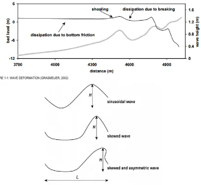
Waves approach the shore deform due to among other shoaling and wave breaking (See Figure 1-1). The deformation of the waves is not only visible on the wave height. The wave shapes also deform as wave approach the shore. Wave become velocity skewed and acceleration skewed as they approach the shore (See Figure 1-2).

Wave breaking can be classified in four categories; in this case there are plunging breaking waves. For this category the value wave similarity parameter is between 0.5 and 3. The wave similarity parameter can be calculated with the wave steepness , the wave height and the wave length (Battjes, 1974):

EQ. 1-1

(11)

[image:11.595.106.517.119.496.2]

MODELING SAND TRANSPORT UNDER BREAKING WAVES 2 FIGURE 1-1: WAVE DEFORMATION (GRASMEIJER, 2002)

FIGURE 1-2: WAVE SKEWNESS AND ASYMMETRY (GRASMEIJER, 2002).

Sediment transport is the movement of particles in the water column. The driving parameter for sediment transport is bed shear stress. Bed shear stress is defined as the bottom friction by water per area. The bottom friction causes lower flow velocities near the bed and it also causes turbulence near the bed responsible for the picking up of sediment (see Figure 1-3).

FIGURE 1-3: SEDIMENT PICK UP AND DEPOSITION

(12)

MODELING SAND TRANSPORT UNDER BREAKING WAVES 3

EQ. 1-2

In which is the depth averaged velocity, is the density of water and is a friction coefficient. The initiation of motion is determined by exceedance of the Shields parameter over the critical Shields parameter:

EQ. 1-3

The Shields parameter is commonly defined as a dimensionless bed shear stress.

1.3 Research objective

The objective of the research is to improve the sediment transport prediction by Delft3D for breaking wave conditions using the SANTOSS formula. The SANTOSS model is not developed to predict the near bed sediment transport under breaking waves (van der A et al., 2013), since it is developed for non-breaking waves. There are currently some suggestions on how to adjust the SANTOSS model for wave-breaking effects. These effects will be tested in Delft3D with the new highly detailed measurement of wave breaking in a flume (van der Zanden et al., 2015). It should be kept in mind that also suspended sediment might be modeled poorly. In that case it would be wiser to improve the suspended sediment predictions.

This introduces a mean to reach this objective; the current SANTOSS model will be validated for the highly detailed measurement on wave breaking in a flume and the results of the SANTOSS model will also be compared with the results of the commonly used net sediment transport model of van Rijn. This is required to complete the objective. In a previous study it seemed that the SANTOSS model within Delft3D predicts the net sediment transport reasonably well (Van der Werf, Veen, Ribberink, & van der Zanden, 2015; Veen, 2014).

1.4 Research questions

Five research questions have been formulated to help achieve the objective mentioned in the previous section. Each research question will be answered in a separate section starting with the first research question in the third section.

1. How do the overall hydrodynamics below breaking waves look in the new Barcelona measurements and how well can Delft3D reproduce these hydrodynamics?

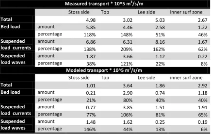
2. What are, according to measurements and Delft3D, the contributions of different transport components (bed-load, suspended load, current- and wave- related components) to the total sediment transport in the breaker zone and how well can Delft3D reproduce these transport components with the SANTOSS and the van Rijn (2007ab)(Bed load and suspended load/concentration) model?

3. How can the differences between Delft3D and the measured transport components be explained?

3.1. Can wrong sediment transport predictions be explained by errors in the modeled overall hydrodynamics (wave height, set-up, undertow and orbital flow skewness/asymmetry)? 3.2. Can sediment transport predictions be improved by changing the near-bed velocity

reference height or by adding bed slope effects in the stand-alone model?

3.3. Can wrong sediment transport predictions be explained by specific effects of wave breaking?

(13)

4. How is it possible to account for wave-breaking effects in the SANTOSS transport model (stand-alone Matlab-model and/or Delft3D)?

4.1. Which model concepts are available?

4.2. How well do they compare with the data and with the current models? 4.3. What is the best (calibrated) concept?

5. How does the SANTOSS model (in Delft3D or Matlab) with improvements for wave-breaking effects perform for other test cases?

1.5 Research approach and reading guideline

1.5.1 General research approach

The SANTOSS model is a model that is currently under construction and the SINBAD project aims at improving the current SANTOSS model with wave-breaking and wave irregularity effects. During this project improvements for breaking wave effects on the SANTOSS model have been tested in a stand-alone Matlab version of the SANTOSS model and within the Delft3D environment. Possible improvements of the SANTOSS model have been tested stand-alone, because possible improvements are easier to implement in Matlab. The Delft3D environment is used as it is a more often used software package to model hydrodynamics and morphodynamics. Another reason for using Delft3D is that it calculates much more than the near-bed sediment transport only, also hydrodynamics and suspended sediment will be calculated.

During this research project measurements from the CIEM wave flume in Barcelona have been compared with model results and differences will be explained. Differences between model results and measurements have al lot of sources. Some of these sources are errors in the measurements, processes that are not well modeled, poor parameter settings or there might be numerical solving problems. This research project aims at approaching of the model results to the measurements of the experiments in the CIEM wave flume in Barcelona. This is done by firstly changing the parameter settings during a calibration and after that by changing the processes in a stand-alone SANTOSS model and in the Delft3D environment.

During this Master Thesis some formulations used in Delft3D and in the SANTOSS model have been adapted. To distinguish adapted formulations from standard formulations, the adapted formulations have been marked with an asterisk.

1.5.2 Research question 1

The first research question is answered in section 3 by first looking at the measured hydrodynamics. The hydrodynamics are explored and different hydrodynamics like wave height; set-up, net currents, orbital velocities, velocity skewness and acceleration skewness have been examined. Secondly the breaking waves in the wave flume have been reproduced in a Delft3D model. The hydrodynamics have been reproduced as well as possible by doing a calibration. The results of this calibration are compared to the measured hydrodynamics. After that, it is determined if the hydrodynamics are reproduced well enough so that it will not influence the sediment transport negatively. It is also examined why difference between the measured hydrodynamics and the modeled hydrodynamics occur.

(14)

suspended sediment and a combined formula for wave related bed- and suspended load and current related bed-load. Since Delft3D requires a current related suspended sediment formula if SANTOSS is used the sediment transport formula of van Rijn (2007b) is used. This gives some overlap since the SANTOSS formula is not tuned to the van Rijn (2007b) suspended sediment transport formula; this is taken into account. Both models have a different distinction between bed-load and suspended load. Therefore, it is important to make a clear distinction between the different sediment transport components. Also, modeled suspended sediment concentrations are compared with the measured sediment concentration, including reference concentrations and sediment diffusivities. This helps assign possibly poorly modeled current related sediment transport to poorly modeled hydrodynamics or sediment concentrations. The second research question, from which the research approach is just discussed, will be answered in section 4.

The third research question, answered in section 5, aims at examining the differences between Delft3D and the measured transport. It is examined whether possible differences are caused by errors in the modeled overall hydrodynamics, if possible difference occur from missing bed slope effects or from the choice for the near-bed velocity reference height and/or if possible differences are caused by specific missing effects of wave breaking. Differences caused by errors in the hydrodynamics will be examined with a stand-alone Matlab version of SANTOSS. Hydrodynamic parameters are not included in the Matlab code because it is a stand-alone model. The hydrodynamics have been inserted manually. The measured hydrodynamics and the Delft3D modeled hydrodynamics have been inserted in this stand-alone Matlab model. The measured bed-load transport is available, this makes including suspended sediment transport unnecessary. The results of the stand-alone SANTOSS models can then be compared to the measurements, in this way it is assessed if errors in the modeled sediment transports are caused by errors in the modeled hydrodynamics. The effect of the bed slopes and the near-bed velocity reference height will also be examined in this section. In this way it is examined if possible differences between sand transport predictions and measurements are due to specific effects of wave breaking. The last part of this research question determines whether it is necessary to improve the current Delft3D models for near-bed transport and/or suspended sediment transport.

The fourth research question answers how it is possible to account for wave-breaking effects in the SANTOSS model. Therefore it is examined which model concepts on breaking wave effects are available. Three of these ideas that are tested are changing the formulations of the wave Reynolds stress, adding turbulence to the orbital velocities and adding turbulence to the Shields parameter (van der Zanden, 2014). The results of the models with improvements for breaking wave effects have been compared with the measurements and with the current models. The stand-alone Matlab model is used since it requires less time to test improvement for wave breaking effects. It is examined which model concept for breaking wave effects works best. This is done by comparing the results of the stand-alone Matlab model with different improvements for wave breaking effects with each other and with the measurements. At last, the best calibrated concept is tested in Delft3D. The near-bed sediment transport modeled with Delft3D including wave breaking effects within the SANTOSS model has been compared to the measurements. Also some morphological computations were done to examine how well DELFT3D predicts the breaker bar. The fourth research question is answered in section 6.

(15)

2 METHODOLOGY

The methodology will firstly give a brief introduction on Delft3D and secondly on the suspension- and bed-load transport. Thirdly the SANTOSS model, on which improvements will be tested, will be introduced. Fourthly the model set-up used in this project will be discussed and at last the CIEM wave flume experiments will be introduced.

2.1 Delft3D

The sand transport will be predicted with a stand-alone Matlab model and within the Delft3D environment. Delft3D is a 3 dimensional software package, which calculates flows, waves, sediment transport and morphological change. It consists of integrated modules which allow the simulation of hydrodynamic flow, computation of the transport of water-borne constituents, short waves generation and propagation, sediment transport and morphological changes, and the modeling of ecological processes and water quality parameters (Lesser, Roelvink, van Kester, & Stelling, 2004). Delft3D solves the unsteady shallow water equations. Delft3D uses a curvilinear grid in which the shallow water equations are solved. It is possible to calculate the sediment transport in Delft3D with a selection of sediment transport formula. A commonly used transport within Delft3D is the van Rijn (2007ab) model, discussed in section 2.1.3 and 2.1.4.

This Master Thesis involves the modeling of waves in Delft3D, it is therefore important to mention that Delft3D does not model individual waves. Delft3D models the forcing of waves through the wave propagation theory (See section 2.1.2).

2.1.1 System of Equations

To solve the numerical model the software packages uses a staggered grid, meaning that the water level points are located at the center of the grid cells and the velocity points are located at the faces of the grid cells (see Figure A-1).

The equations below are valid for a Cartesian rectangular grid (Lesser et al., 2004). The horizontal grid can be separated into -layers or z-layers, the difference is shown in Figure A-2. The thicknesses of these layers are user-defined. Thin layers are mostly used near the bottom and the water surface in the presence of wave while thicker layers are mostly used in the middle of the water column and near the water surface when waves are not present.

The systems of equations that Delft3D handles are the horizontal momentum equations, the continuity equation, the transport equation and a turbulence closure model. The equations are shown in Appendix A.2, first the continuity equations, then the two horizontal momentum equations, the transport equation and some discussion on the turbulence closure model are shown.

2.1.2 Waves

Delft3D is also able to account for wave effects (Deltares, 2014); short waves can be modeled in Deft3D through the wave propagation method calculated using the wave energy. Effects of wave breaking can be included using the roller model. For more extended waves modeling the separate Delft3D-Wave module needs to be applied (Deltares, 2014), this is not relevant for this study. So, only the wave propagation and the Roller model will be discussed here.

Wave propagation

(16)

velocity of the waves. This is equal to the velocity of short waves for shallow areas. Basis of the wave propagation theory is the wave energy balance:

EQ. 2-1

In this formula, E is the wave energy, is the group velocity, the wave direction with respect to the coast, is the wave dissipation due to wave breaking and is the wave dissipation due to bottom friction. The wave dissipation is calculated through the method of Roelvink (1993). The wave energy dissipation due to wave breaking is given by the formulation of Baldock, Holmes, Bunker, & Van Weert (1998).

Roller model

When waves break wave energy will be reduced rapidly and the energy will be transformed into roller energy throughout the roller model in Delft3D. The effect of wave breaking is not well understood, but ignoring the effect is as shown by recent studies not an option (Deltares, 2014). The energy balance for the roller model is shown below:

EQ. 2-2

In this formula C is the wave celerity and is the roller energy dissipation. The energy dissipation due to wave breaking is input for the roller model. The roller energy dissipation has influence on the surface stress.

2.1.3 Suspended sediment model

Suspended sediment transport is of large influence on the total amount of sediment transport. Especially near coasts with fine sediment. Suspended sediment is also important near wave breaking locations where a lot of turbulent mixing occurs.

Suspended sediment concentrations in Delft3D are calculated with the three-dimensional advection diffusion equation for suspended sediment (Deltares, 2014):

EQ. 2-3

In this equation the first term is the change of sediment concentration over time, the second and the third term are the change of sediment advection in the x and the y direction. The fourth term is the change of sediment concentration over depth. The last three terms are the sediment diffusivity in the x, y and z direction.

(17)

[image:17.595.213.411.112.243.2]

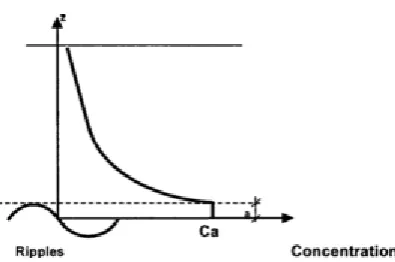
MODELING SAND TRANSPORT UNDER BREAKING WAVES 8 FIGURE 2-1: SUSPENDED SEDIMENT CONCENTRATION PROFILE OF THE VAN RIJN (2007B) METHOD. CA IS THE REFERENCE CONCENTRATION AND THE REFERENCE HEIGHT A.

The reference concentration is calculated with the following formula:

EQ. 2-4

In this formula, for sand,

is the dimensionless particle parameter,

is the median particle size of bed material, is the dimensionless bed-shear stress

parameter given by:

EQ. 2-5

With is the time averaged critical bed shear stress and is the time averaged effective

bed shear stress due to waves and currents. The reference level from EQ. 2-4 is given by:

EQ. 2-6

In this formula is current-related nikuradse roughness height and is the wave-related

nikuradse roughness height. The total sediment transport per unit width is given by the integration of the net current and the sediment concentration between the reference level and the still water level :

EQ. 2-7

2.1.4 Bed load sediment

The bed load sediment transport calculated by van Rijn (2007a) and the SANTOSS transport formula (van der A et al., 2013) will be compared with measurements during this research. Improving the SANTOSS formula is the objective of this research, the SANTOSS formula will be discussed separately in the next section. The van Rijn (2007a) model will be discussed in this section.

(18)

MODELING SAND TRANSPORT UNDER BREAKING WAVES 9 EQ. 2-8

And are herein coefficients with respectively the values 0.5 and 1. Is the sediment density.

Is the critical bed shear stress according to Shields. Is the grain-related bed-shear

stress due to both currents and waves given by:

EQ. 2-9

With is the velocity due to currents and waves at the edge of the wave boundary layer.

Is the grain friction coefficient due to currents and waves at this is given by the following formulation:

EQ. 2-10

In this formula is a coefficient related to relative strength of wave and currents given by . Is a coefficient related to the vertical structure of the velocity profile. And are the current and wave related grain friction based on the grain related roughness

EQ. 2-11

With is the water depth and is the peak orbital diameter near the bed.

In the bed-load transport vector an estimation for suspended sediment caused by wave asymmetry (See Figure 1-2) effects is also present:

EQ. 2-12

With is the wave related suspended transport, is a user defined tuning parameter, is

the phase factor with a value of 0.1 and is the velocity asymmetry factor. is calculated

with the offshore ( ) and onshore ( ) peak orbital velocity. The concentration between van

Rijn's (2007b) reference height and the thickness of the suspension layer near the bed is taken into account to calculate the wave related suspended load. The suspension layer near the bed is given by , with is the near bed sediment thickness layer.

2.2 SANTOSS model

2.2.1 General

The SANTOSS model is a newly developed practical sand transport formula that predicts the near bed net sand transport under non-breaking regular waves (van der A et al., 2013).

(19)

reacts to flow conditions (da Silva, Temperville, & Seabra Santos, 2006). Semi unsteady formulas can also take effect from previous flow conditions on sand transport into account. The SANTOSS model is very useful for cross-shore sand transport under wave dominated conditions. The transport formula is based on the half wave-cycle concept from Dibajnia & Watanabe (1992), which describes the total net transport as the difference between the transported during the positive “crest” half cycle and the negative “trough” half-cycle. Using the sediment transported in the current half-cycle and which is entrained in the previous half cycle phase lag effects can be applied.

The net transport rate is given by the following formula (van der A et al., 2013):

_{EQ. 2-13}

The formula uses non-dimensional bed shear stress as the main forcing parameter. and

are the periods and the acceleration period of the crest and the trough (See Figure 2-2). The sand load entrained during each half wave is given by the following formula:

EQ. 2-14

With is the critical Shields number, which is in the SANTOSS formula calculated according to

Soulsby (1997). The Shields parameter vector is calculated as follows (van der A et al., 2013).

EQ. 2-15

In which the wave current friction factor is calculated as the linear combination of the wave

friction factor and the current friction factor (Ribberink, 1998). The wave Reynolds stress is

a stress contribution due to progressive surface waves (Fredsoe & Deigaard, 1992; Nielsen, 2006). Is the root mean square velocity of a sinusoidal flow and and are the

combined wave-current velocity vectors in the x and the y direction. The velocities are a combination of the orbital velocity of the waves and the current related velocity. The orbital velocity caused by wave will vary over time and over orientation. The orientation of the whole model is in the same direction as the orientation of the waves.

2.2.2 Phase lag

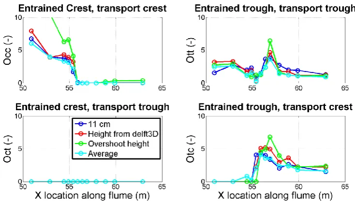
In the SANTOSS formula there are four contributions to the net sand transport (van der A et al., 2013). These are the sediment entrained and transported during the crest ( ) and the trough

( ) period and the sediment entrained in the crest and trough period transported respectively in

the trough ( ) and the crest period ( ) (see Figure 2-2). Phase lag effects can especially be

(20)

MODELING SAND TRANSPORT UNDER BREAKING WAVES 11 FIGURE 2-2: CREST AND TROUGH PERIODS OF OSCILLATORY FLOWS

Phase lag effects are implemented by dividing the sand entrained in the crest ( ) and trough period ( over transport in the current half wave cycle and the next half wave cycle. This is done by a phase lag parameter . The phase lag parameters are calculated with the following formula:

EQ. 2-16

EQ. 2-17

In which is a calibration factor, the ripple height calculated according to O’Donoghue, Doucette, van der Werf, & Ribberink (2006), the sheet flow layer thickness according to

Dohmen-Janssen (1999) and is the sediment settling velocity within the half cycle. The term

with ripple height or the sheet flow layer thickness represents a ratio of the representative stirring height and the sediment settling distance in one half wave cycle.

The terms between the square brackets in EQ. 2-16 and EQ. 2-17 present an effect of progressive waves on the phase lag behavior. The effect is horizontal sediment advection caused by horizontal non-uniformity in the wave field. Kranenburg, Ribberink, Schretlen, & Uittenbogaard (2013) show that this effect leads to a compression of sand during the wave crest and dilution of sand during the wave trough. This causes a net transport in the direction of the wave propagation.

If the phase lag parameter is lower than or equal to 1 there is no phase lag. If exceeds 1 there is a phase lag. The fraction of the sand entrained that will be transported with a phase lag is than . The fraction that is transported in the same half wave period it was entrained is then (van der A et al., 2013).

2.2.3 Flow Regime

(21)

EQ. 2-18

With is the ripple height, is the ripple length, and are parameters depending on respectively the median grain size , and the mobility number and is the orbital excursion

amplitude. The mobility number depends on the flow properties:

EQ. 2-19

With is the peak orbital crest velocity, is the peak orbital trough velocity and is the relative density of the sediment particles. The flow regime is quite important for the direction of the predicted sediment transport. When ripples are present it is most likely that phase lag occurs and the sediment transport will probably be offshore directed. For sheet-flow the sediment transport will probably be onshore directed.

2.2.4 Implementation in Delft3D

The Santoss model has been implemented in Delft3D by Veen (2014). During this implementation it seemed that some conceptual expansion of the SANTOSS model was required. SANTOSS requires intra wave velocities. Intra-wave velocities are not calculated in Delft3D since Delf3D just calculates the forcing by waves. Therefore, Veen (2014) implemented the approximation method of Abreu, Silva, Sancho, & Temperville (2010) by Ruessink, Ramaekers, & Van Rijn (2012) for the intra wave velocities in Delft3D. In this method the orbital flow characteristics are calculated. The velocity skewness and acceleration skewness required for SANTOSS are calculated from these orbital flow characteristics.

Another conceptual expansion is that the calculation for the crest and trough periods and the duration of the acceleration period of the crest and trough (See Figure 3-11) are based on the intra wave velocities. Previously the crest and trough periods were calculated with an approximation method using the peak orbital crest and trough velocity and the acceleration skewness.

2.3 Model set-up

In this section the grid used during the calibration will be shown. Also some initial and boundary conditions will be discussed. At last, some model settings will be discussed in this section.

2.3.1 Grid

The model grid consists of 263 cross-shore grid locations, one grid cell in the alongshore direction and 24 vertical layers. The grid is finest near the location of the breaker bar (~0.2 meter length for one grid cell). Near the boundaries the grid is much coarser (~0.9 meter length of one grid cell). This is a very fine grid, but this is desirable due to detailed measurements and energetic conditions (regular breaking waves, steep breaker bar and sheet flow conditions) The water depth near the open boundary (left side of the grid) is 2.55 meter. The grid is shown in Figure 2-3. The time-step used in the model is 0.06 seconds. This is required to deal with the drying and flooding conditions and corresponding Courant numbers near and at the shore.

(22)

B-2). The model results using 24 and 36 layers are almost equal. Therefore 24 vertical layers will be used for further calculations. The layers thickness is defined as a percentage of the water depth and is as follows: 1%, 1.3%, 1.6%, 2%, 2.4%, 3.1%, 3.8%, 4.8%, 5.8%, 7%, 8.2 %, 9%, 9%, 8.2%, 7%, 5.8%, 4.8%, 3.8%, 3.1%, 2.4%, 2%, 1.6%, 1.3% and 1%.

FIGURE 2-3: GRID DIMENSIONS.

2.3.2 Initial and boundary conditions

Initial conditions and boundary conditions are required to be able to run the model. The initial conditions are conditions that are specified at the start of the model run (t = 0 s). One of these initial conditions is the water level. The initial water level is set uniform to 0 meter. The other initial condition is the sediment concentration in the water column; this is set to 0 kg/m3. During the measurements the water level in the wave flume was at rest. The sediment had the time to settle down; therefore the sediment concentration in the model has to be set to zero as well.

There is an open boundary in the model at location x = 0 m (see Figure 2-3). Waves are generated at the open boundary. The wave period is specified at four seconds and the waves are directed from the open boundary (x = 0) towards the beach. During the measurements the wave height was set by a wave paddle at 0.85 m. During the measurements it seemed that the wave height was not equal to 0.85 m. During the calibration there is accounted for the difference between the target wave height and measured wave height.

2.3.3 Model settings

The grain sizes used in the model are equal to the measured grain sizes. The median grain size (D50) is 246 μm. The 10 percentile grain size (D10) and the 90 percentile grain size (D90) are respectively 154 and 372 μm. The specific density, the density of the sediment with respect to the density of water is equal to 1.65.

(23)

especially important behind the breaker bar and the roughness caused by the breaker bar can be modeled as a roughness caused by megaripples.

Morphodynamic updating has been switched off during the calibration. The bottom used during modeling in Delft3D is fixed to exclude morphodynamic effect. Morphodynamics are an additional complexity during modeling and are not necessarily required to improve the modeling of sediment transport in Delft3D with the SANTOSS model for breaking wave effects. To minimize the effect of bottom development on the measurement only the measurements of the first measurement run on each day has been used (van der Zanden et al., 2015).

2.4 Description of the dataset

The processes under breaking waves are not well understood and therefore new large scale experiments on breaking waves in the CIEM wave flume in Barcelona have been done (van der Zanden et al., 2015). The wave flume is 100 m long and 3 m wide. At one side of the flume a wave paddle is located and at the other side of the wave flume a beach is constructed. With this wave paddle regular breaking waves were generated.

2.4.1 Set-up

The set-up of the experiment is shown in Figure 2-4. The wave paddle is shown on the left and the beach is shown on the right. The waves are breaking at the top of the breaker bar. Measurements are done with a mobile-frame trolley and a profiling trolley. Measurements with the mobile-frame trolley are done every run of 15 minutes. In total six runs of 15 minutes have been done. After every two runs of 15 minutes the whole bed profile has been measured with the profiling trolley. After one day of measurements the mobile-frame trolley is relocated and the bottom profile is restored to the initial bottom profile. The mobile-frame trolley is located at 12 different locations around the breaker bar (see Figure 2-5). In this way very detailed measurements around the breaker bar are available.

FIGURE 2-4: SET-UP OF THE CIEM WAVE FLUME EXPERIENTS (VAN DER ZANDEN ET AL., 2015)

(24)

2.4.2 Regular breaking waves

During the experiment regular waves which break at the top of the breaker bar were generated. The waves had a period of four seconds and the target wave height at the wave paddle was 0.85 meter. The water level near the wave paddle was 2.55 meter. The bottom slope was 1:10 which creates a plunging wave. The results of the measurements for the velocity, the net sediment transport and the suspended sediment transport will be discussed in the next sections.

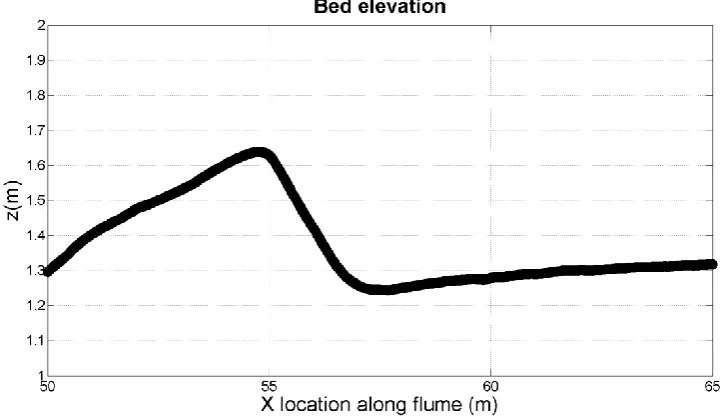
Aim of this experiment was to simulate energetic field conditions, the wave height is relative large compared to the water depth. This caused sheet flow in front of the breaker bar. Sheet flow conditions occur when the flow has a high mobility number. A simplification during the measurements compared to field conditions were the generating of regular breaking waves. Wave regularity causes wave breaking at a steady location. This causes a breaker bar with very steep slope. This is visible in Figure 2-6.

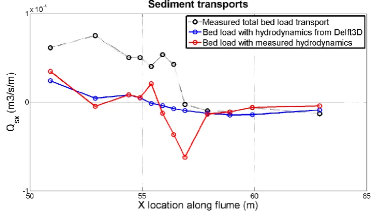
2.4.2.1 Net Sand transport

The net sediment transports are calculated from the bed profile changes measured with the profiling trolley. The difference in bed profile between two successive runs can be used to calculate the net sediment transport with the following formula.

EQ. 2-20

Since the sediment transport at the wave paddle is known and equal to zero the sediment transport at every location in the flume can be calculated. The porosity is assumed to be 0.4.

(25)

MODELING SAND TRANSPORT UNDER BREAKING WAVES 16 FIGURE 2-6: BED EVOLUTION AND NET SEDIMENT TRANSPORT DURING THE CIEM WAVE FLUME EXPERIMENTS (VAN DER ZANDEN ET AL., 2015)

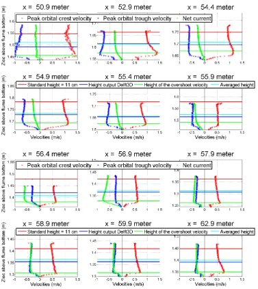
2.4.2.2 Velocities

The velocities are measured with the mobile-frame trolley. Velocities are measured in three dimensions and at three locations at the mobile-frame trolley. The most important location is approximately 11 centimeter above the bed. At every measurement location along the flume the distance between the bed and the lowest velocity measuring device (ADV) was set at 11 centimeter. The measurements results in maximum and minimum orbital velocity. The minimum velocity for the trough and the maximum velocity for the crest are shown in Figure 2-7. The velocities have also been measured with an Acoustic Concentration and Velocity Profiler (ACVP), this device measures the velocity profile from the bed to 15 centimeter above the bed.

(26)

MODELING SAND TRANSPORT UNDER BREAKING WAVES 17 FIGURE 2-7: PHASE-AVERAGED WATER SURFACE ELEVATION AND PHASE AVERAGED HORIZONTAL VELOCITIES FROM T=0 TO T = 15 MINUTES. THE HORIZONTAL BLUE LINE INDICATES THE MEAN CURRENT

2.4.2.3 Suspended sediment

At the mobile-frame trolley there are also some measurement devices that measure the average suspended sediment concentration (TSS device). Together with the undertow this concentration can help calculating the current related suspended sediment transport. In Figure 2-8 the time-averaged suspended sediment concentrations are shown.

FIGURE 2-8: TIME AVERAGED SUSPENDED SEDIMENT CONCENTRATION DURING THE CIEM WAVE FLUME EXPERIMENTS. THE FIRST FIGURE SHOWS THE LOCATION OF THE MEASUREMENTS, THE SECOND FIGURES SHOWS THE SUSPENDED SEDIMENT CONCENTRATION.

(27)

3 MEASURED AND MODELED HYDRODYNAMICS

In this section it will be examined how well Delft3D (see section 2.1 for an introduction of Delft3D) can reproduce the hydrodynamics measured during the CIEM wave flume experiments. Firstly the measured hydrodynamics and the reproduction of those hydrodynamics by Delft3D will be examined. During the reproduction of these hydrodynamics, some improvements for regular breaking waves have been tested; these tests will be discussed as well. Secondly the measured wave skewness and wave asymmetry will be shown and the reproduction by the parameterization method used in Delft3D will be discussed. At last, some conclusions of this section will be drawn.

3.1 Hydrodynamics

The model set-up used during this project is discussed in section 2.3. Delft3D contains user defined calibration parameters and input settings. The goal of the calibration is to approach the results of the measurements with the model predictions by adapting the calibration parameters and the input settings. During the calibration the modeled results will be compared with the measurements. This comparison will be evaluated and as long as the modeled results are not satisfying enough the input calibration parameters and the input settings will be adjusted.

The paper of Giardino, Brière, & van der Werf (2011) and Veen (2014) have been used as a guideline during the calibration of the hydrodynamics. During the calibration of the hydrodynamics the modeled wave height, set-up and undertow are compared with the measurements. Delft3D has a number of calibration parameters that influence the hydrodynamic output. The hydrodynamic parameters in Table 3-1 are the parameters that are used for the hydrodynamic calibration. The physical meaning of the parameters and the formulations in which the parameters are used are discussed as well. The calibrated parameter value has been shown in this table as well.

Next to the calibration parameters there are user defined formulations which are discussed. The implementation of the formulas in the Delft3D model will be discussed firstly.

TABLE 3-1: OPTIMAL HYDRODYNAMIC PARAMETER SETTING

Delft3D has a drying and flooding criterion which determines the minimum water depth required for computations. Due to a large number of vertical layers Delft3D cannot work with the hydrodynamics on such a small scale near area which successively drying and flooding. If the drying and flooding criterion is too low, water levels will vary due to computational errors near the drying and flooding area. The drying and flooding criterion is therefore set to 0.2 meter. When the

Parameter

Description

Symbol

Value

Hs

Wave height at wave paddle

0.80 m

Fwee

Bottom friction factor

0 Gamdis

Wave breaking index

0.58 Alfaro

Roller dissipation coefficient

6 F_lam

Breaker Delay

F_lam

0 Betaro

Rollers lope parameter

0.2 Vicouv

Bankground horizontal eddy viscosity

_{0 m}

2

_/s

Vicoww

Background vertical eddy viscosity

_{0 m}

2

_/s

Alfa

Reflection parameter

0

(28)

water depth at certain locations is lower than 0.2 m, then Delft3D will not perform computations for those locations.

3.1.1 Formulations

In the turbulent closure schemes there is accounted for increased roughness effects due to waves. The additional bed shear stress is added to the roughness height. In Delft3D there are different formulations which can calculate this additional bed shear stress. The wave stress formula of van Rijn, Walstra, & Ormondt (2004) have been used. This wave stress formula predicted the undertow best.

Delft3D has four different turbulence closure models which can be used. Turbulence and space varying viscosity is very important for predicting the strong undertow. The k-epsilon turbulence closure models predict the undertow best at most locations. Therefore this closure model has been used.

3.1.2 Wave height

The wave heights are measured with Resistance Wave Gauges (RWGs) and Pore Pressure Transducers (PPTs). There were two kinds of PPTs, those located at the wall at different location in the wave flume and the PPT located at the measurement frame. The wave heights were averaged over all measurement runs. Error bars have been included to indicate errors due to difference between runs.

The wave heights measured at the mobile frame were not as reliable as other measured wave heights and those wave heights have therefore been excluded from this research. The measured wave heights are shown in Figure 3-1.

The wave height in the roller model in Delft3D is determined by the linear wave theory. In the linear wave theory the wave height is calculated from the wave energy.

EQ. 3-1

In this formula is the short wave energy, is the specific density of water, is the acceleration gravity and is the root mean square wave height. Since there are regular

waves, the wave averaged wave heights do not change over time. So the short wave energy formulation changes to:

*

EQ. 3-2

The wave energy balance in Delft3D is dependable on energy change over the 2 horizontal directions as shown in EQ. 2-1. During the measurements the wave energy only changes over one direction. In the Delft3D model this direction is the x direction. Also the angle of the wave ray with respect to the coast line was zero during the measurements. This reduces the energy balance to:

EQ. 3-3

The wave energy dissipation is given by the parameterization of Baldock et al. (1998):

(29)

With is the roller dissipation coefficient (Alfaro), the water density, the gravitational

acceleration, the peak frequency, the maximum wave height and the root mean

square wave height.

The parameterization of Baldock et al. (1998) is developed for irregular waves. During the calibration there are regular waves. Therefore the formula for energy dissipation due to breaking waves has been changed to a formula applicable for regular waves proposed by Van Rijn & Wijnberg (1996).

*

EQ. 3-5

With is parameter indicating wave breaking, is 1 when waves break and is 0 when waves are not breaking. Waves break when the relative wave height is larger than the wave breaking index _.

Applying just the conditions mentioned above seemed not suitable (See Appendix C.1). Therefore another condition has been implemented based on the measured decreasing wave height. A criterion has been added to the source code, waves continue breaking as long as the wave height during the next step is higher than a relative depth (reldep parameter in Delft3D). This relative depth has been extracted from the measurements and is set to 0.35 meter. This results in the following wave breaking conditions:

* EQ. 3-6

This transition from breaking to non-breaking and the adaptation of the source code is explained in Appendix C.1. The reasoning behind the changes to the source code is explained as well. The effect of different energy dissipation due to wave breaking models on the wave height is shown in Figure C-1.

With the formulation for the energy dissipation due to wave breaking changed it is much easier to better predict the steep decrease of the wave height due to wave breaking. The steepness of the slope is determined by the roller dissipation coefficient (Alfaro). The default value for Alfaro is 1 and the advised range of Alfaro is between 0.5 and 2. An Alfaro of 6 was required to predict the energy dissipation due to wave breaking well (Figure D-1). A lower value for Alfaro reduces the wave energy dissipation due to wave breaking; the decrease in wave height would be underestimated using a lower value for Alfaro. So it seems that the wave breaking model used still underestimates the energy dissipation due to wave breaking.

The maximum wave height from EQ. 3-5 is given by:

EQ. 3-7

(30)

stop breaking (Roelvink, Meijer, Houwman, Bakker, & Spanhoff, 1995). A breaker delay is not required since the location of wave breaking has been calibrated with the wave breaking index.

The energy dissipation due to bottom friction is given by (Stive & Vriend, 1994; Svendsen, 1984):

EQ. 3-8

In this formula is a bottom friction parameter and is the orbital velocity of the waves. The

energy dissipation due to bottom friction has been excluded, even though the wave height is overestimated offshore of the breaker bar. If the bottom friction would have been included the peak wave height in front of the breaker location would be lower than the current peak wave height. The calibration, with the parameter values as mentioned above, results in the wave heights shown in Figure 3-1.

FIGURE 3-1: CALIBRATED WAVE HEIGHTS. THE LINE SHOWS THE CALIBRATED WAVE HEIGHTS, ASTERISK SHOW THE MEASURED WAVE HEIGHT WITH PPT’S AND THE PLUS SIGN SHOW THE MEASURED WAVE HEIGHT WITH THE RWG’S.

3.1.3 Set-up

The set-up is just as the wave height derived from the RWG and PPT water level measurements. The set-up measured with the PPT at the mobile frame has been excluded from the results because of the unreliability of these measurements (See section 3.1.2). The set-down at the beginning of the flume, where no set-down is to be expected, is larger than zero. This suggests that either the set-down is overestimated or that the water level was not exactly 2.55 meter. Around and behind the breaker bar from X = 50 m and onshore set-up occurs.

The set-up in Delft3D can be influenced by the energy dissipation of the roller model. Energy of the roller will be transferred to the water column in the energy balance of the roller model. The energy balance of the roller model is derived from EQ. 2-2 and is as follows:

EQ. 3-9

(31)

EQ. 3-10

The parameter (Betaro) in this formula is important for determining the set-up and the

undertow. This parameter determines the wave energy transferred from the roller model to the underlying water, this parameter barely has effect on the wave height. This makes it possible to separately calibrate the wave height and the set-up.

The set down is underestimated for the largest part of the wave flume (see Figure 3-2). The set-down in front of the wave breaking seems impossible to obtain. Only by using uncommon values for the certain parameters the set-up in the breaker region was modeled quite well, but this caused fluctuation in the set-down in front of the wave breaking location and this also causes poor predictions of the undertow. The set-up as shown causes the best prediction of the undertow. To obtain this set-up the background vertical and horizontal eddy viscosity (Vicouv and Vicoww) have been set to zero. The roller slope parameter (Betaro) has been set to 0.2, this was especially important for the undertow. Also the set-up experiences effects from changing the roller slope parameter. A roller slope parameter value of 0.2 caused a quite good prediction of the set-up and it causes an as well as possible prediction of the undertow.

FIGURE 3-2: CALIBRATED SET-UP. THE LINE SHOWS THE CALIBRATED SET-UP, RED ASTERISK SHOW THE MEASURED SET-UP WITH PPT’S AND THE BLUE PLUS SIGN SHOW THE MEASURED SET-UP WITH THE RWG’S.

3.1.4 Undertow

The undertow compensates for the onshore directed mass transport under waves and under rollers called the Stokes drift due to respectively waves and rollers. The undertow is extracted from intra-wave velocity profiles measured with Acoustic Doppler Velocimeters (ADVs) and Acoustic Concentrations and Velocity Profilers (ACVPs). The ADVs measure the velocity at 11, 37 and 84 centimeter above the bed. The ACVPs measure the velocity profile from the bed to 15 centimeter above the bed with a vertical resolution of 0.15 centimeter. Both the ADVs and the ACVPs show quite reliable results. This is confirmed by the fact that the measurement obtained by the lowest ADV show almost equal results to the measurement obtained by the ACVP.

(32)

Figure 3-3. For some locations the ACVPs measure the undertow below the bed level. This has two reasons. The first reason is that during the measurement sometimes ripples appear and disappear, therefore the local bed level increases and decreases. The second reason is that the bed level is measured with a different measurement device; this causes differences in the measured bed level.

As mentioned in section 3.1.3 the undertow showed a strong relationship with the set-up. The parameter Betaro is important for the set-up and the undertow (See Figure D-3). The parameter settings to obtain the set-up shown above also predict the most optimal undertow. A lower value than 0.2 causes a better prediction on top of the breaker bar (x = 52.9 to x = 55.9 m), but this causes a worse prediction at the lee side of the breaker bar (x = 56.4 to x = 57.9 m). A higher value than 0.2 cause’s inversed results compared to using a lower value for Betaro.

One parameter was changed to improve the undertow after improving the set-up. This is the reflection parameter; the reflection parameter alpha makes the open offshore water level boundary less reflective for disturbances that occur at the start of the computation. This reflection parameter damps small disturbances in the model out. It also damps out the undertow. Therefore the reflection parameter has been set to zero. To deal with the small disturbances, output has been averaged over the model time.

The best modeled undertow is shown in Figure 3-3. In front of the breaking location and behind the breaking location the undertow is predicted quite well. But it is very hard to predict the undertow near the breaker location well. The undertow is underestimated near the breaker locations (X locations 55.9 until 57.9 m). All parameters with possible effect on the prediction of the undertow have been varied. Improvements of the predicted undertow due to these variations where either not found or the predicted undertow improved for some locations and worsened for the other locations (See Appendix C for source code adaptations and Appendix D parameter adaptation).

Some adaptations to the source code have been done to test improvements for the prediction of the net current. Looking at the results it seems that the Stokes mass flux is underestimated behind the breaking location (x = 56.4 to x = 57.9 m). Therefore the Stokes drift due to rollers has been made depth dependable according to Uchiyama, McWilliams, & Shchepetkin (2010). After testing the depth dependable Stokes drift it seemed that for some location the undertow was predicted better (From x = 55.9 to x = 57.9 m) and for the other locations the predictions of the undertow got worse (See Figure C-3). The derivation of the depth dependable Stokes drift due to rollers and the results obtained after using this equation are shown in Appendix C.2. When using the depth dependable stokes drift due to rollers the undertow for most locations became worse, therefore this equation for the Stokes drift has not been used.

(33)

MODELING SAND TRANSPORT UNDER BREAKING WAVES 24 FIGURE 3-3: MEASURED AND MODELED UNDERTOW. THE UNDERTOW IS MEAUSRED WITH THE ADV AND THE AVCP DEVICES. THE NET CURRENT AT THE WAVE BOUNDARY LAYER (UNET AT WBL) IS SHOWN WHILE THE NET CURRENT AT THIS HEIGHT IS INPUT FOR THE SANTOSS MODEL.

(34)

3.1.5 Net Vertical currents

The net vertical currents are important for the determinion of the suspension concentrations. Therefore the measured vertical currents have been compared to the modeled vertical currents in Figure 3-5. There are some uncertainties in the measured vertical currents. The vertical currents measured with the ACVPs do not match with the measured vertical current of the lowest ADV for some locations. The vertical currents seem to be downwards directed in front of and at the top of the breaker bar, while the direction suddenly changes to upward from x = 55.9 m and onshore.

The modeled vertical current are almost always upwards directed. Onshore of the breaker bar, for x is larger than 57.9 meter, the vertical currents almost decreased to zero. For some locations the vertical currents show a local decrease of the vertical current. This is due to the mass flux due to rollers which is applied in the top part of the water column.

(35)

3.2 Wave skewness and asymmetry

Veen (2014) implemented the approximation method of Abreu, Silva, Sancho, & Temperville (2010) by Ruessink, Ramaekers, & Van Rijn (2012) for the orbital flow velocity skewness and asymmetry in Delft3D. The results of this approximation method will be compared with the measured wave skewness and asymmetry. Firstly the approximation method will be discussed, then the measurements and the model results will be discussed and then the suitability of the approximation method of Ruessink et al. (2012) will be discussed.

3.2.1 Approximation method

With the wave number, calculated with the linear wave theory, the wave height and the water depth the Ursell number (Ursell, 1953) can be calculated.

EQ. 3-11

According to Ruessink et al. (2012) a Boltzmann sigmoid function should be used to determine the relation between the Ursell number and the total measure of non-linearity B. Also the phase

can be determined from the Ursell number.

EQ. 3-12

EQ. 3-13

p1 To p6 are calibration parameters with advised values of p1 = 0, p2 = 0.857, p3 = -0.471, p4 = 0.297, p5 = 0.815 and p6 = 0.672. The total measure of non-linearity can be used to calculate the parameter of skewness or nonlinearity with the following formula (Malarkey & Davies, 2012):

EQ. 3-14

Since there is not a single solvable relation between the total measure of linearity and the parameter of skewness or nonlinearity . Veen (2014) used basic fitting with a third order polygon to calculate r from a given . The result of that basic fitting is given with the formula below. The basic fitting result in an R squared of 0.9998.

EQ. 3-15

The wave form parameter can be calculated from the phase with the following formula (Malarkey & Davies, 2012):

EQ. 3-16

(36)

EQ. 3-17

EQ. 3-18

The corresponding velocity skewness ( ) and the acceleration skewness or velocity asymmetry ( ) which is input for the SANTOSS model can respectively be described by:

EQ. 3-19

EQ. 3-20

The wave skewness and wave asymmetry are calculated with:

EQ. 3-21

EQ. 3-22

Is the orbital velocity amplitude, is the standard deviation of the orbital velocity amplitude and is a Hilbert transform of the orbital velocity amplitude.

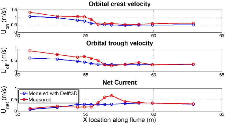
3.2.2 Measurements and modeling results

The modeled results with the hydrodynamics calibrated in section 3.1 and the advised parameter settings for the Boltzmann Sigmoid function and the measurements are shown for respectively the peak orbital velocities, the flow velocity skewness and flow velocity asymmetry in Figure 3-6, Figure 3-7 and Figure 3-8.

Modeling sand transport under breaking waves

MODELING SAND TRANSPORT UNDER

BREAKING WAVES

PREFACE

ABSTRACT

TABLE OF CONTENTS

1

INTRODUCTION

2

METHODOLOGY

3

MEASURED AND MODELED HYDRODYNAMICS

Parameter

Description

Symbol

Value

Hs

Wave height at wave paddle

0.80 m

Fwee

Bottom friction factor

0

Gamdis

Wave breaking index

0.58

Alfaro

Roller dissipation coefficient

6

F_lam

Breaker Delay

F_lam

0

Betaro

Rollers lope parameter

0.2

Vicouv

Bankground horizontal eddy viscosity

0 m

/s

Vicoww

Background vertical eddy viscosity

0 m

/s

Alfa

Reflection parameter

0

_{0 m}

_/s

_{0 m}

_/s